
CNN-Based Fault Detection for Smart Manufacturing †


Abstract
:1. Introduction
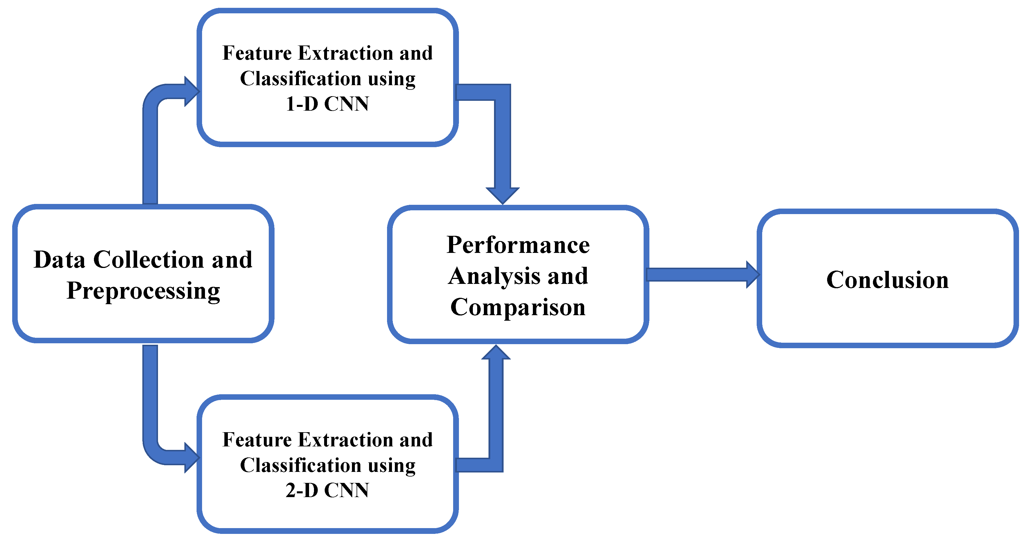
1.1. Methodology
1.2. Contribution and Organization
2. Related Theory and Work
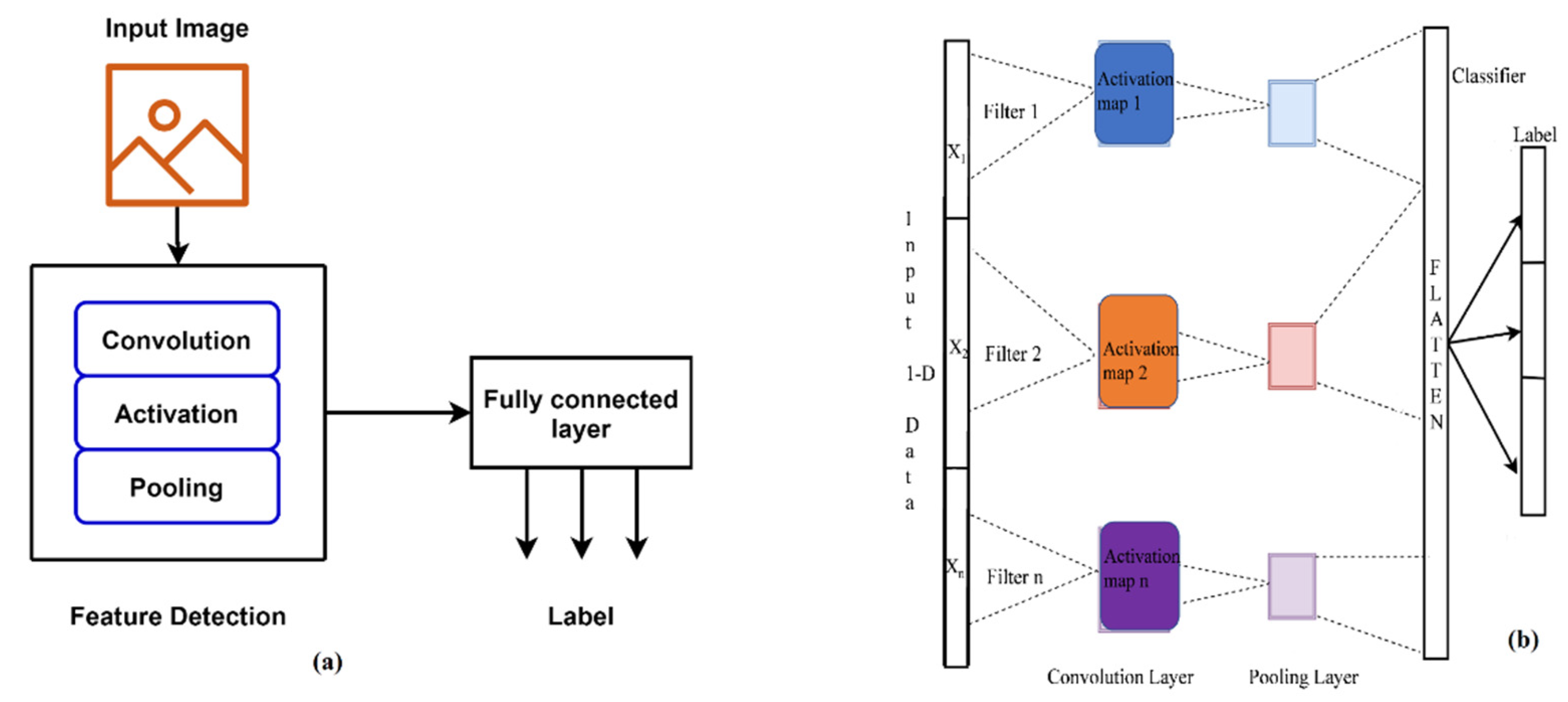
2.1. Related Theory
- Convolutional Neural Networks (CNNs)
- B.
- SoftMax Classifier
- C.
- Batch Normalization
- D.
- ReLU
2.2. Related Work
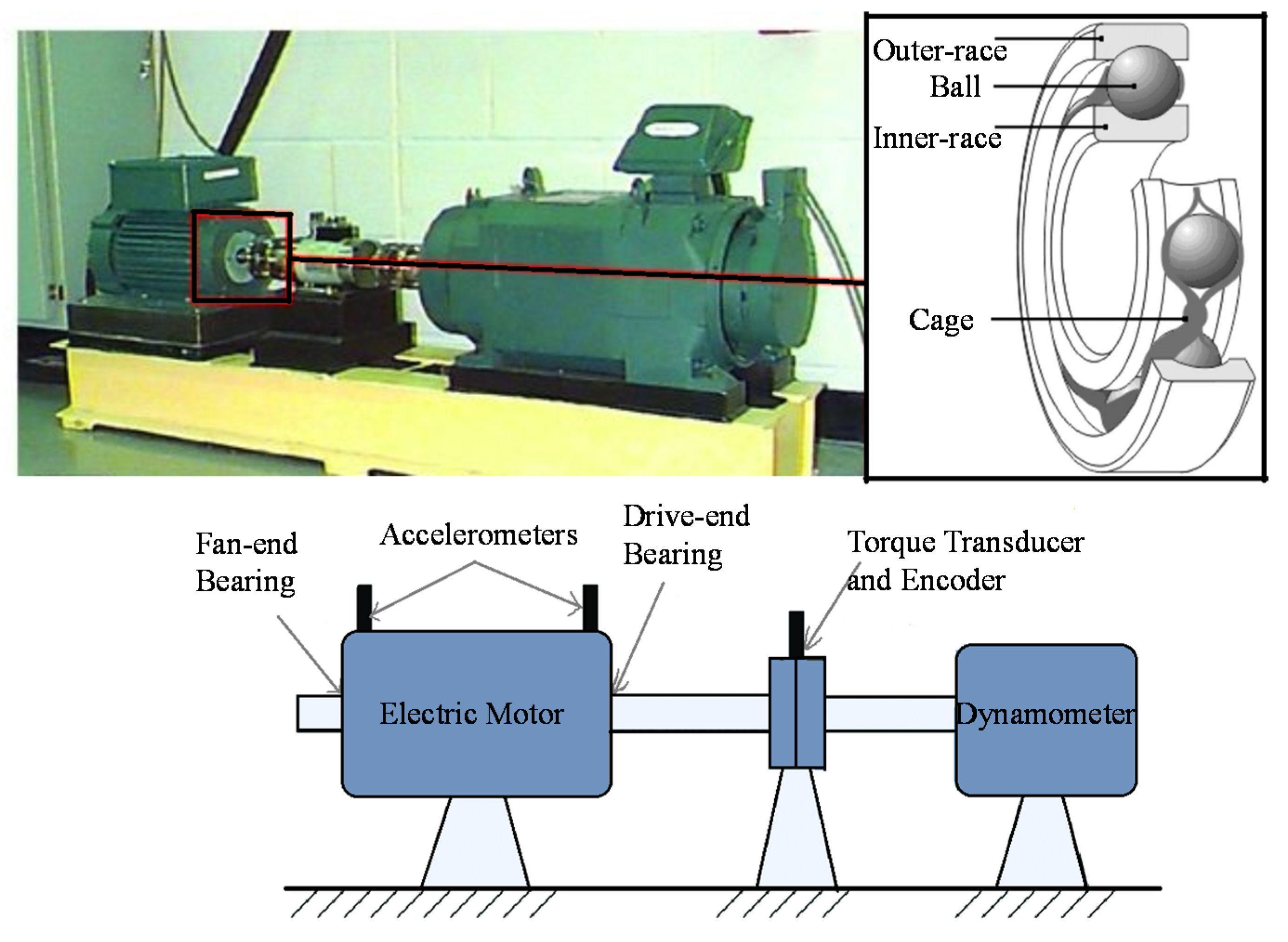
3. Experimental Analysis
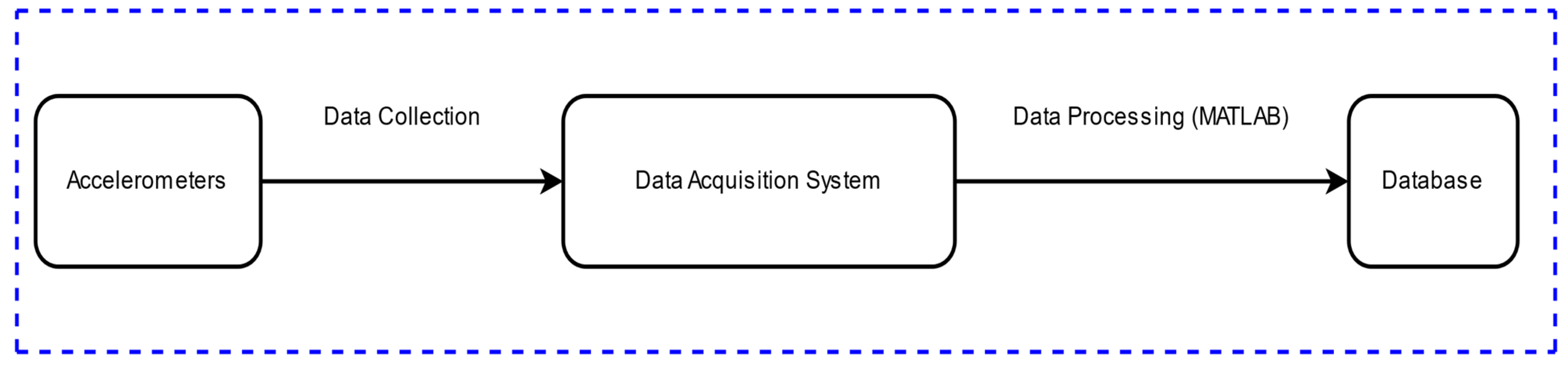
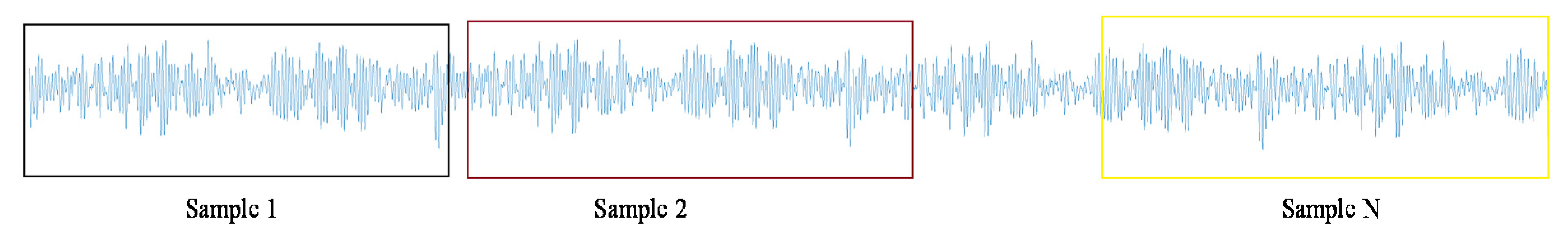
3.1. Data Analysis and Pre-Processing
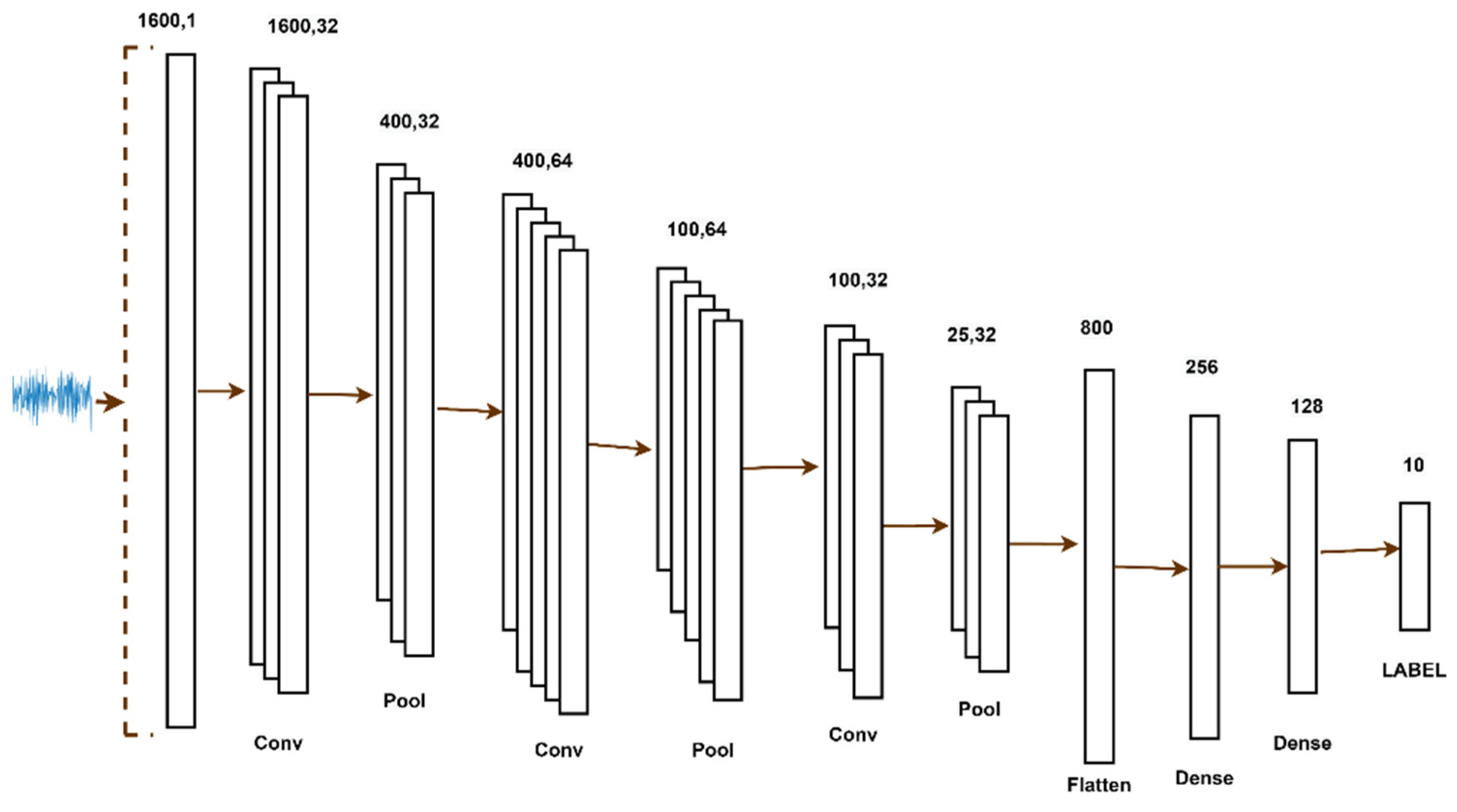
3.2. Feature Extraction and Classification Using 1-D CNN
3.3. Sensitivity Analysis and Model Stability
4. Compared Method
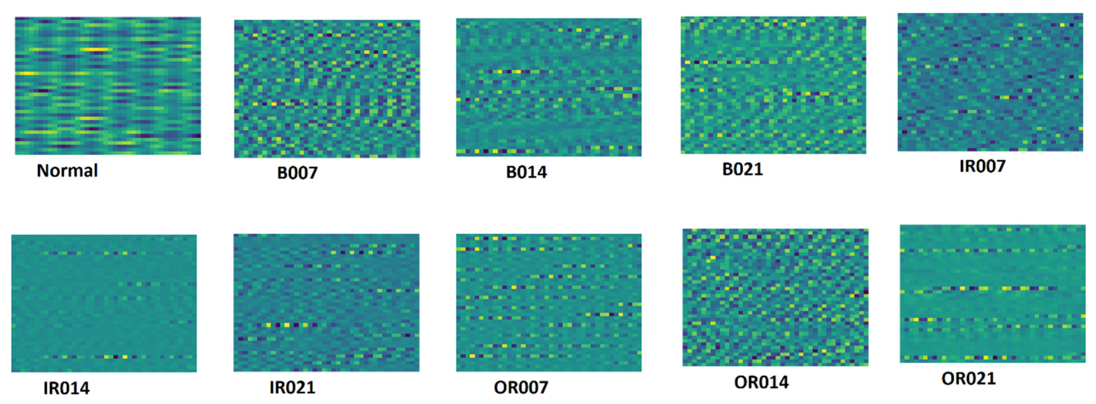
4.1. Image (2-D Representation) Construction from 1-D Vibration Data
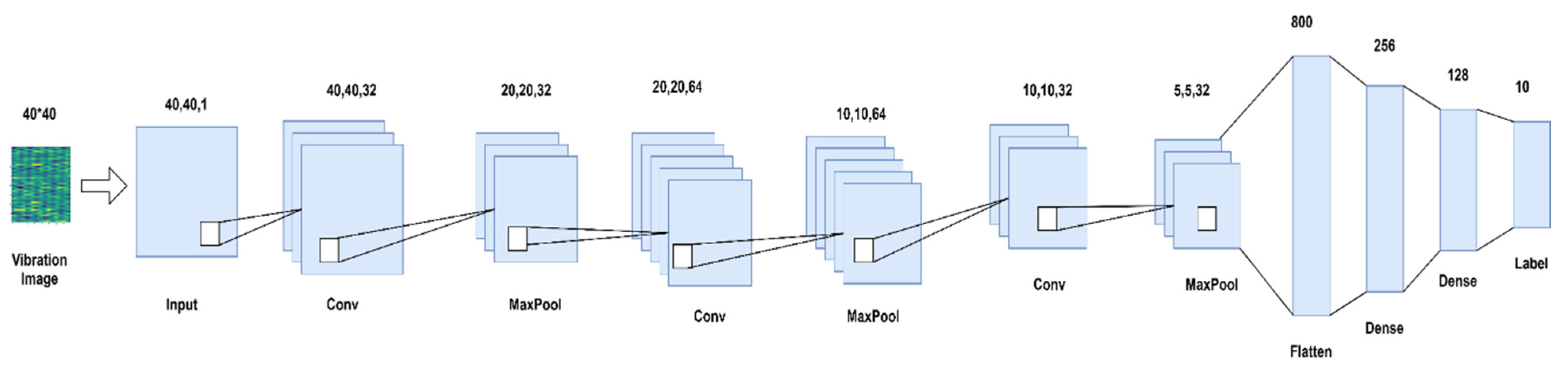
4.2. Comparison Using 2-D CNN
4.3. Comparison of the Proposed Model with Some Other Published Works
5. Discussion and Conclusions
Author Contributions
Funding
Institutional Review Board Statement
Informed Consent Statement
Data Availability Statement
Acknowledgments
Conflicts of Interest
Abbreviations
| 1-D | One-Dimensional |
| 2-D | Two-Dimensional |
| ANN | Artificial Neural Network |
| CWRU | Case Western Reserve University |
| CNN | Convolutional Neural Network |
| DE | Drive End |
| DL | Deep Learning |
| FE | Fan End |
| GPU | Graphics Processing Unit |
| IR | Inner-Race |
| k-NN | k-Nearest Neighbor |
| ML | Machine Learning |
| NS | Normal State |
| OR | Outer-Race |
| PCA | Principal Component Analysis |
| RMS | Root Mean Square |
| ReLU | Rectified Linear Unit |
| SVD | Singular Value Decomposition |
| SVM | Support Vector Machine |
References
- Neupane, D.; Seok, J. Bearing Fault Detection and Diagnosis Using Case Western Reserve University Dataset With Deep Learning Approaches: A Review. IEEE Access 2020, 8, 93155–93178. [Google Scholar] [CrossRef]
- Zhang, S.; Zhang, S.; Wang, B.; Habetler, T.G. Deep Learning Algorithms for Bearing Fault Diagnosticsx—A Comprehensive Review. IEEE Access 2020, 8, 29857–29881. [Google Scholar] [CrossRef]
- Neupane, D.; Seok, J. Deep Learning-Based Bearing Fault Detection Using 2-D Illustration of Time Sequence. In Proceedings of the 2020 International Conference on Information and Communication Technology Convergence (ICTC), Jeju, Korea, 21–23 October 2020; pp. 562–566. [Google Scholar] [CrossRef]
- Huang, W.; Cheng, J.; Yang, Y. Rolling Bearing Fault Diagnosis and Performance Degradation Assessment under Variable Operation Conditions Based on Nuisance Attribute Projection. Mech. Syst. Signal Process. 2019, 114, 165–188. [Google Scholar] [CrossRef]
- Neupane, D.; Kim, Y.; Seok, J. Bearing Fault Detection Using Scalogram and Switchable Normalization-Based CNN (SN-CNN). IEEE Access 2021, 9, 88151–88166. [Google Scholar] [CrossRef]
- Boudiaf, A.; Moussaoui, A.; Dahane, A.; Atoui, I. A Comparative Study of Various Methods of Bearing Faults Diagnosis Using the Case Western Reserve University Data. J. Fail. Anal. Prev. 2016, 16, 271–284. [Google Scholar] [CrossRef]
- Wen, X.; Lu, G.; Liu, J.; Yan, P. Graph Modeling of Singular Values for Early Fault Detection and Diagnosis of Rolling Element Bearings. Mech. Syst. Signal Process. 2020, 145, 106956. [Google Scholar] [CrossRef]
- Yang, S.; Liu, Z.; Lu, G. Early Change Detection in Dynamical Bearing Degradation Process Based on Hierarchical Graph Model and Adaptive Inputs Weighting Fusion. IEEE Trans. Ind. Inform. 2021, 17, 3186–3196. [Google Scholar] [CrossRef]
- Wang, T.; Lu, G.; Yan, P. A Novel Statistical Time-Frequency Analysis for Rotating Machine Condition Monitoring. IEEE Trans. Ind. Electron. 2020, 67, 531–541. [Google Scholar] [CrossRef]
- Smith, W.A.; Randall, R.B. Rolling Element Bearing Diagnostics Using the Case Western Reserve University Data: A Benchmark Study. Mech. Syst. Signal Process. 2015, 64–65, 100–131. [Google Scholar] [CrossRef]
- Zhang, S.; Zhang, S.; Wang, B.; Habetler, T.G. Machine Learning and Deep Learning Algorithms for Bearing Fault Diagnostics—A Comprehensive Review. In Proceedings of the 2019 IEEE 12th International Symposium on Diagnostics for Electrical Machines, Power Electronics and Drives (SDEMPED), Toulouse, France, 27–30 August 2019. [Google Scholar] [CrossRef]
- Ince, T.; Kiranyaz, S.; Eren, L.; Askar, M.; Gabbouj, M. Real-Time Motor Fault Detection by 1-D Convolutional Neural Networks. IEEE Trans. Ind. Electron. 2016, 63, 7067–7075. [Google Scholar] [CrossRef]
- Neupane, D.; Seok, J. A Review on Deep Learning-Based Approaches for Automatic Sonar Target Recognition. Electronics 2020, 9, 1972. [Google Scholar] [CrossRef]
- Feng, Z.; Liang, M.; Chu, F. Recent Advances in Time—Frequency Analysis Methods for Machinery Fault Diagnosis: A Review with Application Examples. Mech. Syst. Signal Process. 2013, 38, 165–205. [Google Scholar] [CrossRef]
- Bhandari, S.; Kim, H.; Ranjan, N.; Zhao, H.P.; Khan, P. Optimal Cache Resource Allocation Based on Deep Neural Networks for Fog Radio Access Networks. J. Internet Technol. 2020, 21, 967–975. [Google Scholar]
- Zappone, A.; Di Renzo, M.; Debbah, M. Wireless Networks Design in the Era of Deep Learning: Model-Based, AI-Based, or Both? IEEE Trans. Commun. 2019, 67, 7331–7376. [Google Scholar] [CrossRef] [Green Version]
- Ranjan, N.; Bhandari, S.; Zhao, H.P.; Kim, H.; Khan, P. City-Wide Traffic Congestion Prediction Based on CNN, LSTM and Transpose CNN. IEEE Access 2020, 8, 81606–81620. [Google Scholar] [CrossRef]
- Lecun, Y.; Bottou, L.; Bengio, Y.; Ha, P. Gradient-Based Learning Applied to Document Recognition. Proc. IEEE 1998, 86, 2278–2324. [Google Scholar] [CrossRef] [Green Version]
- Krizhevsky, A.; Sutskever, I.; Hinton, G.E. ImageNet Classification with Deep Convolutional Neural Networks. Adv. Neural Inf. Process. Syst. 2012, 25, 1097–1105. [Google Scholar] [CrossRef]
- He, Z.; Shao, H.; Zhong, X.; Zhao, X. Ensemble Transfer CNNs Driven by Multi-Channel Signals for Fault Diagnosis of Rotating Machinery Cross Working Conditions. Knowl.-Based Syst. 2020, 207, 106396. [Google Scholar] [CrossRef]
- Oh, J.W.; Jeong, J. Convolutional Neural Network and 2-D Image Based Fault Diagnosis of Bearing without Retraining. In ICCDA 2019: Proceedings of the 2019 3rd International Conference on Compute and Data Analysis; Association for Computing Machinery: New York, NY, USA, 2019; pp. 134–138. [Google Scholar] [CrossRef]
- Valle, R. Hands-On Generative Adversarial Networks with Keras: Your Guide to Implementing Next-Generation Generative Adversarial Networks; Packt Publishing Ltd.: Birmingham, UK, 2019. [Google Scholar]
- Waziralilah, N.F.; Abu, A.; Lim, M.H.; Quen, L.K.; Elfakharany, A. A Review on Convolutional Neural Network in Bearing Fault Diagnosis. In MATEC Web of Conferences, Engineering Application of Artificial Intelligence Conference 2018 (EAAIC 2018); EDP Sciences: Les Ulis, France, 2019; Volume 255. [Google Scholar] [CrossRef] [Green Version]
- O’Shea, K.; Nash, R. An Introduction to Convolutional Neural Networks. arXiv 2015, arXiv:1511.08458. [Google Scholar]
- Westlake, N.; Cai, H.; Hall, P. Detecting People in Artwork with CNNs. Lect. Notes Comput. Sci. 2016, 9913, 825–841. [Google Scholar] [CrossRef] [Green Version]
- Kiranyaz, S.; Ince, T.; Hamila, R.; Gabbouj, M. Convolutional Neural Networks for Patient-Specific ECG Classification. In Proceedings of the 2015 37th Annual International Conference of the IEEE Engineering in Medicine and Biology Society (EMBC), Milan, Italy, 25–29 August 2015; pp. 2608–2611. [Google Scholar]
- Kiranyaz, S.; Avci, O.; Abdeljaber, O.; Ince, T.; Gabbouj, M.; Inman, D.J. 1D Convolutional Neural Networks and Applications—A Survey. Available online: http://arxiv.org/abs/1905.03554 (accessed on 20 September 2021).
- Liu, W.; Wen, Y.; Yu, Z.; Yang, M. Large-Margin Softmax Loss for Convolutional Neural Networks. arXiv 2016, 2, 7. [Google Scholar]
- Lei, Y.; Jia, F.; Lin, J.; Xing, S.; Ding, S.X. An Intelligent Fault Diagnosis Method Using Unsupervised Feature Learning Towards Mechanical Big Data. IEEE Trans. Ind. Electron. 2016, 63, 3137–3147. [Google Scholar] [CrossRef]
- Di, Z.; Shao, H.; Xiang, J. Ensemble Deep Transfer Learning Driven by Multisensor Signals for the Fault Diagnosis of Bevel-Gear Cross-Operation Conditions. Sci. China Technol. Sci. 2020, 64, 481–492. [Google Scholar] [CrossRef]
- Tiara, D.; Muhammad Amir Masruhim, R.S. Batch Normalization. In Data Mining: Practical Machine Learning Tools and Techniques; Morgan Kaufmann: Burlington, MA, USA, 2017; p. 436. [Google Scholar] [CrossRef]
- Sun, J.; Yan, C.; Wen, J. Intelligent Bearing Fault Diagnosis Method Combining Compressed Data Acquisition and Deep Learning. IEEE Trans. Instrum. Meas. 2018, 67, 185–195. [Google Scholar] [CrossRef]
- Shao, H.; Jiang, H.; Zhang, X.; Niu, M. Rolling Bearing Fault Diagnosis Using an Optimization Deep Belief Network. Meas. Sci. Technol. 2015, 26. [Google Scholar] [CrossRef]
- Jiang, W.; Cheng, C.; Zhou, B.; Ma, G.; Yuan, Y. A Novel GAN-based Fault Diagnosis Approach for Imbalanced Industrial Time Series. Available online: http://arxiv.org/abs/1904.00575 (accessed on 7 June 2021).
- Jiang, H.; Li, X.; Shao, H.; Zhao, K. Intelligent Fault Diagnosis of Rolling Bearings Using an Improved Deep Recurrent Neural Network. Meas. Sci. Technol. 2018, 29. [Google Scholar] [CrossRef]
- Wang, R.; Jiang, H.; Li, X.; Liu, S. A Reinforcement Neural Architecture Search Method for Rolling. Measurement 2019, 154, 107417. [Google Scholar] [CrossRef]
- Kaya, Y.; Kuncan, M.; Kaplan, K.; Minaz, M.R.; Ertunç, H.M. Classification of Bearing Vibration Speeds under 1D-LBP Based on Eight Local Directional Filters. Soft Comput. 2020, 24, 12175–12186. [Google Scholar] [CrossRef]
- Kaya, Y.; Kuncan, M.; Kaplan, K.; Minaz, M.R.; Ertunç, H.M. A New Feature Extraction Approach Based on One Dimensional Gray Level Co-Occurrence Matrices for Bearing Fault Classification. J. Exp. Theor. Artif. Intell. 2020, 33, 161–178. [Google Scholar] [CrossRef]
- Xu, Y.; Tian, W.; Zhang, K.; Ma, C. Application of an Enhanced Fast Kurtogram Based on Empirical Wavelet Transform for Bearing Fault Diagnosis. Meas. Sci. Technol. 2019, 30, 035001. [Google Scholar] [CrossRef]
- Kuncan, M. An Intelligent Approach for Bearing Fault Diagnosis: Combination of 1D-LBP and GRA. IEEE Access 2020, 8, 137517–137529. [Google Scholar] [CrossRef]
- Kaplan, K.; Kaya, Y.; Kuncan, M.; Minaz, M.R.; Ertunç, H.M. An Improved Feature Extraction Method Using Texture Analysis with LBP for Bearing Fault Diagnosis. Appl. Soft Comput. 2020, 87, 106019. [Google Scholar] [CrossRef]
- Eren, L. Bearing Fault Detection by One-Dimensional Convolutional Neural Networks. Math. Probl. Eng. 2017, 2017, 8617315. [Google Scholar] [CrossRef] [Green Version]
- Li, X.; Zhang, W.; Ding, Q.; Sun, J.Q. Intelligent Rotating Machinery Fault Diagnosis Based on Deep Learning Using Data Augmentation. J. Intell. Manuf. 2018, 31, 433–452. [Google Scholar] [CrossRef]
- Xia, M.; Li, T.; Xu, L.; Liu, L.; De Silva, C.W. Fault Diagnosis for Rotating Machinery Using Multiple Sensors and Convolutional Neural Networks. IEEE/ASME Trans. Mechatron. 2018, 23, 101–110. [Google Scholar] [CrossRef]
- Zhang, W.; Peng, G.; Li, C. Bearings Fault Diagnosis Based on Convolutional Neural Networks with 2-D Representation of Vibration Signals as Input. MATEC Web Conf. 2017, 95, 1–5. [Google Scholar] [CrossRef] [Green Version]
- Hoang, D.T.; Kang, H.J. Rolling Element Bearing Fault Diagnosis Using Convolutional Neural Network and Vibration Image. Cogn. Syst. Res. 2019, 53, 42–50. [Google Scholar] [CrossRef]
- Li, X.; Zhang, W.; Ding, Q. Neurocomputing A Robust Intelligent Fault Diagnosis Method for Rolling Element b Earings Base d on Deep Distance Metric Learning. Neurocomputing 2018, 310, 77–95. [Google Scholar] [CrossRef]
- Case Western Reserve University Bearing Data Center. Available online: https://csegroups.case.edu/bearingdatacenter/home (accessed on 22 August 2021).
- González-Muñiz, A.; Díaz, I.; Cuadrado, A.A. DCNN for Condition Monitoring and Fault Detection in Rotating Machines and Its Contribution to the Understanding of Machine Nature. Heliyon 2020, 6, e03395. [Google Scholar] [CrossRef] [PubMed]
- Cholletrançois, F. Keras. Available online: https://keras.io/ (accessed on 5 July 2021).
- Abadi, M.; Barham, P.; Chen, J.; Chen, Z.; Davis, A.; Dean, J. Tensorflow: A System for Large-Scale Machine Learning. Available online: https://www.tensorflow.org/ (accessed on 5 July 2021).
- GeForce RTX 2080 Ti Graphics Card|NVIDIA. Available online: https://www.nvidia.com/en-us/geforce/graphics-cards/rtx-2080-ti/ (accessed on 27 July 2021).


| Dataset | Motor Speed (rpm) | Load (hp) | Fault Condition | |||||||||
|---|---|---|---|---|---|---|---|---|---|---|---|---|
| Ball Fault | IR Fault | OR Fault | Normal | |||||||||
| A | 1772 | 1 | B007 | B014 | B021 | IR007 | IR014 | IR021 | OR007@6 | OR014@6 | OR021@6 | None |
| B | 1750 | 2 | B007 | B014 | B021 | IR007 | IR014 | IR021 | OR007@6 | OR014@6 | OR021@6 | None |
| C | 1730 | 3 | B007 | B014 | B021 | IR007 | IR014 | IR021 | OR007@6 | OR014@6 | OR021@6 | None |
| Dataset | Train Set | Test Set | Validation Set |
|---|---|---|---|
| 48k_DE_Load1 (A) | 1499 | 714 | 167 |
| 48k_DE_Load2 (B) | 1908 | 909 | 213 |
| 48k_DE_Load3 (C) | 1908 | 909 | 213 |
| D (A/B/C) | 5317 | 2532 | 591 |
| Layers | 1-D CNN | 2-D CNN | ||
|---|---|---|---|---|
| Output Shape | Parameters | Output Shape | Parameters | |
| Input | (None, 1600,1) | 0 | (None, 40, 40, 1) | 0 |
| Conv2D | (None, 1600, 32) | 320 | (None, 40, 40, 32) | 320 |
| MaxPool2D | (None, 400, 32) | 0 | (None, 20, 20, 32) | 0 |
| Conv2D | (None, 400, 64) | 18,496 | (None, 20, 20, 64) | 18,496 |
| MaxPool2D | (None, 100, 64) | 0 | (None, 10, 10, 64) | 0 |
| Conv2D | (None, 100, 32) | 18,464 | (None, 10, 10, 32) | 18,464 |
| MaxPool2D | (None, 25, 32) | 0 | (None, 5, 5, 32) | 0 |
| Flatten | (None, 800) | 0 | (None, 800) | 0 |
| Dense | (None, 256) | 205,056 | (None, 256) | 205,056 |
| Dense | (None, 128) | 32,896 | (None, 128) | 32,896 |
| Classification | (None, 10) | 1290 | (None, 10) | 1290 |
| Total Parameters: 276,522 | Total Parameters: 276,522 | |||
| Dataset | Precision | Recall | f1-Score |
|---|---|---|---|
| A | 0.9932 | 0.9932 | 0.9932 |
| B | 0.9920 | 0.9920 | 0.9920 |
| C | 0.9946 | 0.9946 | 0.9946 |
| D | 0.9949 | 0.9949 | 0.9949 |
| Model | Dataset | Training Accuracy | Testing Accuracy | Validation Accuracy | Average Time Taken/Sample | Loss | |||
|---|---|---|---|---|---|---|---|---|---|
| Train | Test | Train | Test | Validation | |||||
| 1-D CNN | A | 100% | 99.38% | 99.33% | 119 µs | 72 µs | 2.0740e-07 | 0.0201 | 0.0068 |
| 2-D CNN | A | 100% | 96.27% | 96.0% | 168 µs | 79 µs | 8.6794e-07 | 0.2451 | 0.1609 |
| 1-D CNN | B | 100% | 99.34% | 99.53% | 111 µs | 66 µs | 9.9591e-08 | 0.0884 | 0.0117 |
| 2-D CNN | B | 100% | 97.14% | 96.24% | 140 µs | 63 µs | 3.1614e-07 | 0.2553 | 0.2013 |
| 1-D CNN | C | 100% | 99.45% | 99.53% | 111 µs | 63 µs | 2.2180e-08 | 0.0644 | 0.0130 |
| 2-D CNN | C | 100% | 97.92% | 97.18% | 115 µs | 62 µs | 2.9165e-07 | 0.2042 | 0.2614 |
| 1-D CNN | D | 100% | 99.49% | 99.83% | 110 µs | 58µs | 3.3937e-06 | 0.0130 | 0.0132 |
| 2-D CNN | D | 100% | 98.14% | 97.80% | 107 µs | 59 µs | 1.1997e-05 | 0.0997 | 0.0845 |
| Article Reference | Model | Accuracy |
|---|---|---|
| [46] | 2-D CNN using vibration image | 97.74% |
| [42] | 1-D CNN | 97.1% |
| [44] | 2-DCNN-based approach with multiple sensor fusion | 99.41% using 2 sensors 98.35% with 1 sensor |
| [47] | CNN-based deep distance metric learning method | 99.34% for sample length of 8192 |
| Our Model | 1-D CNN | 99.34% to 99.49% for 4 different datasets |
Publisher’s Note: MDPI stays neutral with regard to jurisdictional claims in published maps and institutional affiliations. |
© 2021 by the authors. Licensee MDPI, Basel, Switzerland. This article is an open access article distributed under the terms and conditions of the Creative Commons Attribution (CC BY) license (https://creativecommons.org/licenses/by/4.0/).
Share and Cite
Neupane, D.; Kim, Y.; Seok, J.; Hong, J. CNN-Based Fault Detection for Smart Manufacturing . Appl. Sci. 2021, 11, 11732. https://doi.org/10.3390/app112411732
Neupane D, Kim Y, Seok J, Hong J. CNN-Based Fault Detection for Smart Manufacturing . Applied Sciences. 2021; 11(24):11732. https://doi.org/10.3390/app112411732
Chicago/Turabian StyleNeupane, Dhiraj, Yunsu Kim, Jongwon Seok, and Jungpyo Hong. 2021. "CNN-Based Fault Detection for Smart Manufacturing " Applied Sciences 11, no. 24: 11732. https://doi.org/10.3390/app112411732
APA StyleNeupane, D., Kim, Y., Seok, J., & Hong, J. (2021). CNN-Based Fault Detection for Smart Manufacturing . Applied Sciences, 11(24), 11732. https://doi.org/10.3390/app112411732