Bituminous Mixtures Experimental Data Modeling Using a Hyperparameters-Optimized Machine Learning Approach

Abstract

This study introduces a machine learning approach based on Artificial Neural Networks (ANNs) for the prediction of Marshall test results, stiffness modulus and air voids data of different bituminous mixtures for road pavements. A novel approach for an objective and semi-automatic identification of the optimal ANN’s structure, defined by the so-called hyperparameters, has been introduced and discussed. Mechanical and volumetric data were obtained by conducting laboratory tests on 320 Marshall specimens, and the results were used to train the neural network. The k-fold Cross Validation method has been used for partitioning the available data set, to obtain an unbiased evaluation of the model predictive error. The ANN’s hyperparameters have been optimized using the Bayesian optimization, that overcame efficiently the more costly trial-and-error procedure and automated the hyperparameters tuning. The proposed ANN model is characterized by a Pearson coefficient value of 0.868.

1. Introduction

The different types of bituminous mixtures (BMs) used for road pavements have to be properly designed as mixtures made of aggregates and bitumen, to withstand traffic loads and climate conditions. Unsuitable mechanical characteristics and volumetric properties of bituminous mixtures may lead to various types of distress in road pavements, generally comprising cracks due to fatigue or low temperature, permanent deformations, stripping, etc. Such failure modes decrease the service life of the pavement and represent serious safety issues for road users. As a result, it is important to properly characterize the mechanical behavior of mixes with respect to their composition to allow a performance-based optimization during the mix design phase [1,2,3]. Experimental methods, which require expensive laboratory tests and skilled technicians, are currently used to evaluate the bituminous mixtures’ performance [4,5,6,7,8,9]. Consequently, any modification of the mixtures’ composition, in terms of bitumen type or content, rather than of aggregate gradation, requires new laboratory tests with an increase in time and costs of the design process.

In recent years, many researchers have devoted their efforts to the problem of defining a mathematical or numerical model of BMs’ mechanical behavior, which could quickly elaborate a reliable prediction of the bituminous mixture’s response. To develop predictive equations, two main types of procedures can be used, namely, advanced constitutive modeling methods rather than statistical or data science approaches. Although the mechanistic constitutive methods allow a rational and in-depth analysis of the material response to be performed [10,11,12,13,14,15,16,17], statistical or machine learning approaches are gaining considerable success in the academic community due to the good reliability of their predictions [18,19,20,21], even if they are not physically based. Nevertheless, it has also been reported that statistical regressions of experimental data can produce less accurate predictions than machine learning methods, specifically with regard to Artificial Neural Networks (ANNs) [22,23,24,25,26,27]. Recently, Lam et al. [28] have found that a multiple regression analysis (coefficient of determination, R², equal to 0.790) is less reliable than an ANN approach (R² = 0.925) searching the analytical model to infer compressive strength of roller-compacted concrete pavement from steel slags aggregate and fly ash levels replacing cement.

The ANNs simulate simplified models of human brain: their computing power derive from the number of connections established between artificial neurons, fundamental computing units, and their main function is to map patterns between input and output from a representative experimental sample, mimicking the biological learning process. Such neural models are basically based on a nonlinear fitting approach, neither physical nor mechanistic, to correlate experimental data; the mathematical framework has already been widely discussed, e.g., by Baldo et al. [29]. In recent years, an increased number of researchers have used ANNs in many civil engineering applications, producing impressive results even with regards to the evaluation of road pavements’ characteristics and performance. Tarefder et al. [30] developed a four-layer feed-forward neural network to correlate mix design parameters and BM samples performance in terms of permeability. Ozsahin and Oruc [31] constructed ANN-based models to determine the relationship between the resilient modulus of emulsified BMs and its affecting factors such as curing time, cement addition level, and residual bitumen content. Tapkın et al. [32] presented an application of ANN for the prediction of repeated creep test results for polypropylene-modified BMs. Accurate predictions (R² between 0.840 and 0.970) of the fatigue life of BMs under various loading and environmental conditions were also produced [33,34]. Ceylan et al. [35] discussed the accuracy and robustness of ANN-based models for estimating the dynamic modulus of hot mixes: such models exhibit significantly higher prediction accuracy (also at the input domain boundaries), less prediction bias and better understanding of the influences of temperature and mixture composition than their regression-based counterparts. Recently, Le et al. [36] developed an advanced hybrid model, as it is based both on ANNs and optimization technique, to accurately predict the dynamic modulus of Stone Mastic Asphalt (R² = 0.985); also, they use the proposed model to evaluate and discuss the effects of temperature and frequency on the mechanical parameter. Similarly, Ghorbani et al. [37] used a simple ANN approach for modeling experimental test results and examining the impact of different features on the properties of construction and demolition waste, such as the reclaimed asphalt pavement.

Although the documented research has attempted to introduce new approaches to an empirical–mechanical mix design, the Marshall approach is still widely adopted in many laboratories [38,39,40,41,42,43,44]. Tapkın et al. [45] have verified the possibility of applying ANNs for the prediction of Marshall test results of BMs. The proposed NN model uses the physical properties of standard Marshall specimens to predict the Marshall stability (MS), flow (MF) and Marshall Quotient values obtained at the end of mechanical tests. Ozgan [46] has studied the effects of varying temperatures and exposure times on the stability of BMs and modeled the test data by using a multilayer ANN. Conversely, Mirzahosseini et al. [23] have validated the efficiency of the multilayer perceptron ANNs for the assessment of the rutting potential of dense BMs: the flow number of Marshall specimens has been correlated to the aggregate and bitumen contents, percentage of voids in mineral aggregate, MS and MF. The mechanical characteristics of the bituminous mixtures depend on the volumetric properties as well as the bitumen content. Such parameters have to meet the limits, set by the current local specifications, for the pavement layer interested from the intervention. Nevertheless, voids in mineral aggregate, voids filled with bitumen and air voids (AV) are determined with a specific test (EN 12697-8), which requires additional time and costs. Khuntia et al. [47] have proposed a neural network model that uses the quantities of bitumen and aggregate in Marshall specimens to predict the MS, MF value and AV obtained from the tests. Likewise, Zavrtanik et al. [48] have used ANNs to estimate air void content in several types of BMs produced according to EN 13108-1. Anyway, the literature presented has in common the need to provide the road engineer with an algorithm that can provide accurate predictions of empirical parameters related to BMs, without the need for sophisticated, time-consuming and expensive laboratory testing.

Despite the fact that ANNs have successfully provided predictive equations to quicken the empirical Marshall mix design, such computational models were usually based on a neural network structure set a priori by the research engineer and trained on a random subset of the available data sample. In case of a relatively small data set, such a practice may involve the risk of leaving out some relevant trends from the training set and leading to a variable prediction error, measured on the validation set, due to data sample variability and selected ANN architecture [49]. These issues can be avoided if an efficient model selection and appropriate data partition are performed. In particular, the search for the optimal network architecture, one of the most difficult tasks in ANN studies, consists of tuning the model settings, called hyperparameters, that yield the best performance score on the validation set. Applications of the trial-and-error procedure, as random or grid search, to find the optimal hyperparameters of a machine learning algorithm for a given predictive modeling problem can be found in the relevant literature [23,24]. Nevertheless, Baldo et al. [50,51] have highlighted the limits of such a time-consuming approach and applied a statistical technique of data partitioning, called k-fold Cross Validation, that allows a more accurate estimation of a model’s performance.

An efficient hyperparameters tuning approach, in contrast to random or grid search, is the Bayesian optimization, which has become popular in recent years [52]. Given that evaluating the performance function score for different hyperparameters is extremely expensive, the Bayesian approach builds a probabilistic model, called “surrogate”, mapping hyperparameters of past evaluations to a probability of a score on the performance function and uses such a model to find the next set of promising hyperparameters (i.e., that optimize the surrogate function) to evaluate the actual performance function [53,54].

This paper aimed to develop an autonomous and impartial procedure of neural model selection for predictive modeling problems of bituminous mixtures’ mechanical behavior, using the Bayesian optimization method, that would replace the more costly trial-and-error procedure. In particular, the ANN approach was used to analyze stiffness modulus (ITSM), MS, MF and AV content of 320 Marshall specimens tested at the Highway Engineering Laboratory of the Thessaloniki Aristotle University. The experimental database includes different types of bitumen and aggregate and covers a wide range of bitumen contents and aggregate gradations. In addition, both laboratory- and plant-prepared mixtures were used and their production site was considered among the feature’s variables of the proposed NN model; it correlates mechanical and volumetric properties, collected by means of laboratory tests, to fundamental characteristics of bituminous mixtures, such as bitumen content (% by weight of mix), filler-to-bitumen ratio (%), type of bitumen and aggregate as well as maximum nominal grain size.

The innovative aspect of the presented research is the application of state-of-the-art procedures in the machine learning domain (namely, k-fold Cross Validation and Bayesian optimization) that allow researchers and engineers to solve the problems of classical neural network applications in bituminous mixtures’ behavior modeling. However, the procedure is not intended to replace the experimental method for mixture characterization, but to integrate it with a predictive algorithm that allows the road engineer to improve the mix design process, reducing time and operational costs. The major drawback of the proposed approach is that its proper implementation requires human resources with specific skills, such as machine learning expertise, and large training data sets covering the diversity of BMs materials.

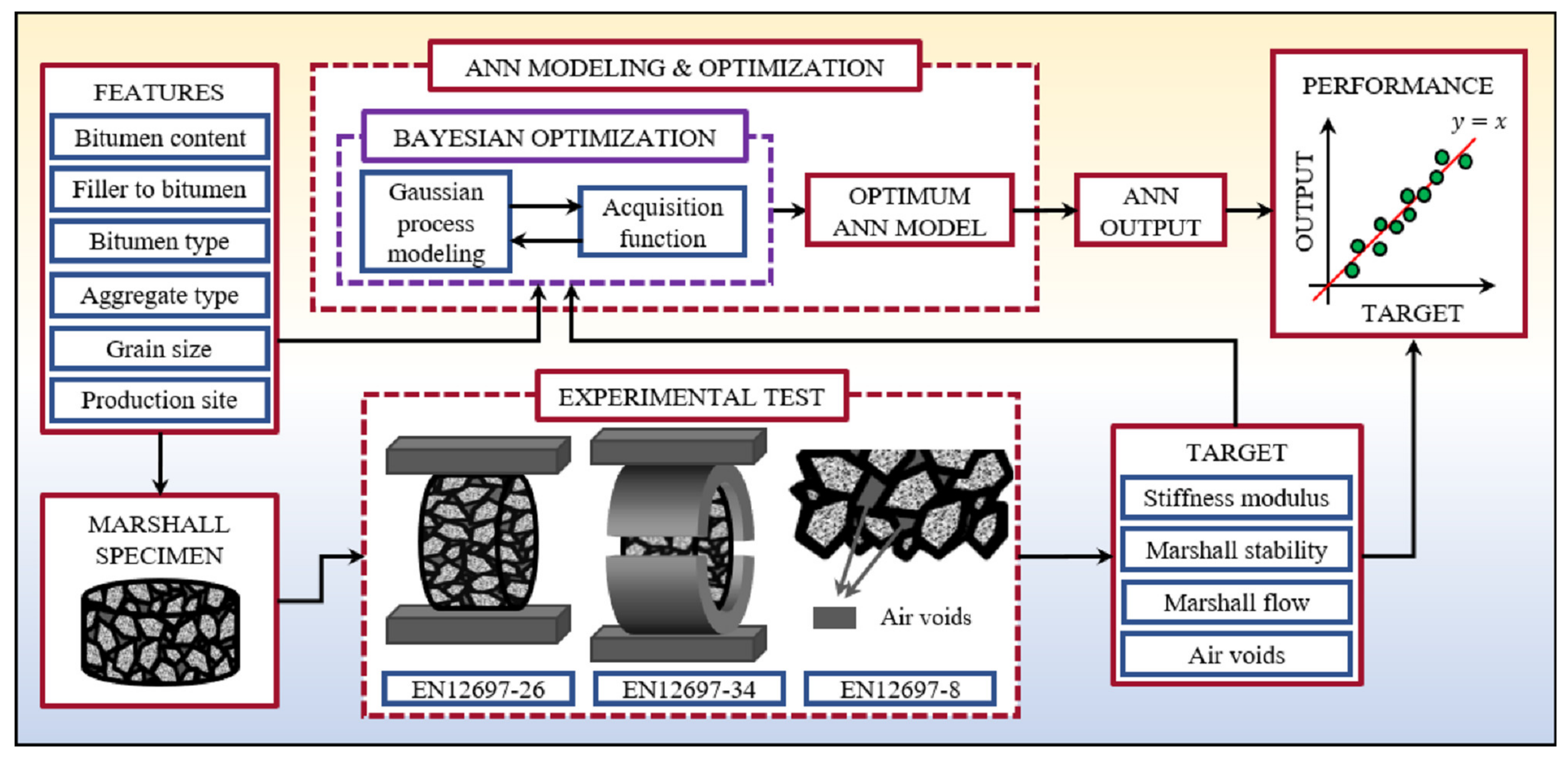
2. Materials and Experimental Design

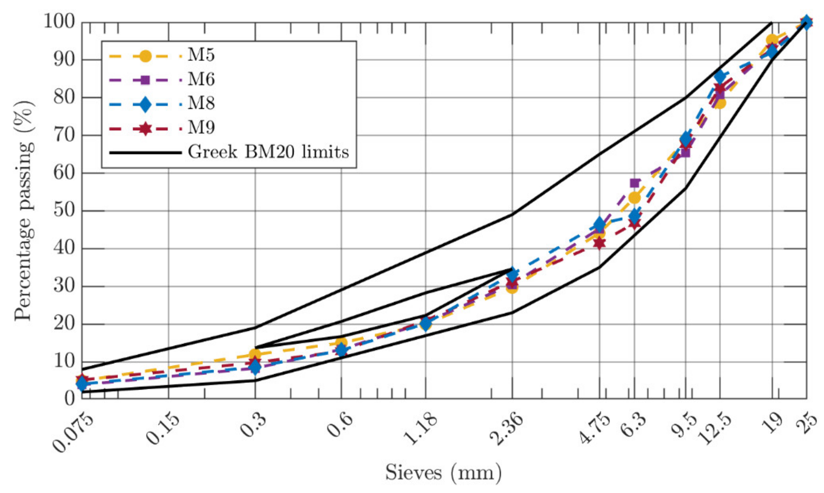
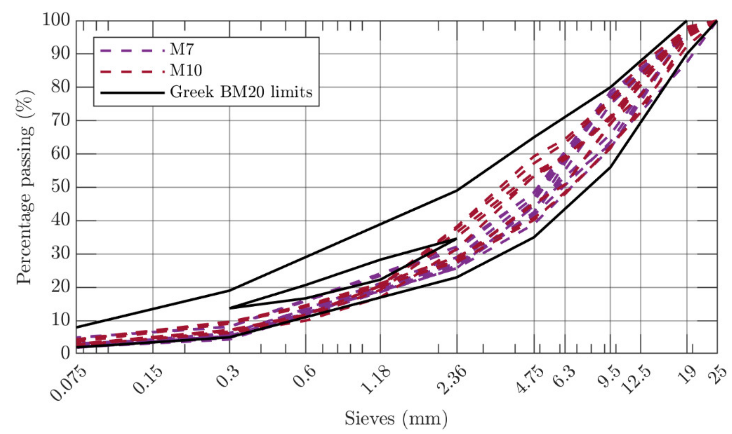
Note that 320 Marshall specimens, having a diameter of 100 mm and an average thickness of 63.7 mm, were produced, both in laboratory and in plant, according to the impact compactor method of test EN 12697-30. These mixtures, designed as part of a research project carried out at the Aristotle University of Thessaloniki, were characterized by different contents of bitumen and aggregate gradations. Aggregates represent the lithic skeleton of a bituminous mixture, while the bitumen is the component binding the aggregate grains together.

2.1. Materials

The aggregates employed were limestone- or diabase-type crushed stones with maximum nominal size of 20 mm or 12.5 mm: the calcareous sedimentary aggregate came from the same Greek quarry, while the mafic igneous one from three different local quarries. To control the physical properties of the aggregates, several tests were conducted. The obtained results are presented in

Table 1. Aggregate properties.

Property	Aggregate Type
	Limestone	Diabase
Los Angeles coeff. (%), EN 1097-2	29	25
Polished stone value (%), EN 1097-8	-	55 to 60
Flakiness index (%), EN 933-3	23	18
Sand equivalent (%), EN 933-8	79	59
Methylene blue v. (mg/g), EN 933-9	3.3	8.3

.

The bituminous mixtures composed of aggregates with maximum nominal size of 12.5 mm (BM12.5) belong to the category “binder course”, while the ones characterized by maximum nominal size of the aggregates equal to 20 mm (BM20) to the “base course” category. In this research, 27 aggregate gradations were considered to meet the gradation limits for binder and base course, set by the current Greek specifications. In each mix category, there are various types of compositions related to the aggregate’s maximum nominal size: for lab-prepared mixtures, 4 types of gradations were used to fit the limits for BM12.5 and 4 types for the BM20. The remaining ones concern BM20 mixtures prepared in plant and correspond to different production days. Figure 1, Figure 2 and Figure 3 show the grading curves involved.

The standard 50/70 penetration bitumen was used in the preparation of 129 Marshall specimens, while the remaining 191 were produced utilizing a bitumen modified in the laboratory with styrene–butadiene–styrene polymers (SBS). The two types of bitumen were tested to ensure that their physical properties were compliant with specific acceptance requisites. The characteristics of bituminous binders are reported in

Table 2. Bitumen properties.

Property	Bitumen Type
	50/70	Modified
Penetration (0.1 × mm), EN1426	64	45
Softening point (°C), EN1427	45.6	78.8
Elastic recovery (%), EN 13398	-	97.5
Fraas breaking point (°C), EN 12593	−7.0	−15.0

. No aging process was performed on bituminous mixtures.

2.2. Experimental Design

The Marshall samples were produced with a bitumen percentage between 3.8% and 6.0% (by weight of mix), and in number equal to three for each bitumen content adopted.

Table 3. Number and codes of Marshall specimens.

Maximum Size (mm)	Aggregate Type	Bitumen Type	Production Site	Mixture ID	Specimens
12.5	Limestone	50/70	Laboratory	M1	30
12.5	Limestone	Modified	Laboratory	M2	30
12.5	Diabase	50/70	Laboratory	M3	30
12.5	Diabase	Modified	Laboratory	M4	30
20	Limestone	50/70	Laboratory	M5	39
20	Limestone	Modified	Laboratory	M6	30
20	Limestone	Modified	Plant	M7	41
20	Diabase	50/70	Laboratory	M8	30
20	Diabase	Modified	Laboratory	M9	30
20	Diabase	Modified	Plant	M10	30

summarizes the number of specimens produced for each combination of bitumen and aggregate; abbreviations coding the mixtures are also reported.

Among the mechanical parameters of bituminous mixtures, the ITSM allows a rational performance-based characterization of the mixes to be performed [4,55]. Therefore, the ITSM test (Figure 4) was executed on all BM samples using the standard testing conditions, defined by EN 12697-26 (temperature of 20 °C, target deformation fixed at 5 μm, and rise time equal to 124 ms). Subsequently, considering that the Marshall parameters are still widely used in road pavement design [38,39,40,41,42,43,44,45], MS and MF were evaluated for the bituminous mixtures produced, according to EN 12697-34. Finally, the specimens’ volumetric characteristics have been determined applying EN 12697-8. The test results are reported in Table S1; such experimental data have been already discussed in previous papers [29,50].

Table 4. Statistical information about Marshall specimens.

Mixture ID	Parameter	Minimum Value	Maximum Value	Mean Value	Standard Deviation
M1	ITSM (MPa)	3756	5554	4556.43	567.93
	MS (kN)	7.71	12.17	9.93	1.09
	MF (mm)	1.99	4.70	3.18	0.84
	AV (%)	1.77	6.37	3.99	1.37
M2	ITSM (MPa)	3628	5142	4345.50	486.50
	MS (kN)	8.74	14.00	11.35	1.73
	MF (mm)	2.00	4.20	3.20	0.57
	AV (%)	2.20	6.29	4.18	1.23
M3	ITSM (MPa)	3812	5942	4804.10	725.03
	MS (kN)	10.30	15.20	12.88	1.53
	MF (mm)	2.00	5.00	3.35	0.95
	AV (%)	1.49	8.91	5.22	2.38
M4	ITSM (MPa)	4035	6293	5076.17	759.06
	MS (kN)	11.60	16.43	13.62	1.42
	MF (mm)	2.20	5.00	3.40	0.92
	AV (%)	1.33	8.36	5.05	2.18
M5	ITSM (MPa)	3215	4919	4252.26	502.24
	MS (kN)	8.91	14.86	11.37	1.51
	MF (mm)	2.18	4.60	3.15	0.50
	AV (%)	2.17	6.75	4.28	1.16
M6	ITSM (MPa)	3907	6043	5243.10	538.97
	MS (kN)	10.40	13.99	11.81	1.21
	MF (mm)	2.24	4.16	3.24	0.40
	AV (%)	1.68	5.21	3.49	1.08
M7	ITSM (MPa)	3103	6399	5065.34	906.93
	MS (kN)	6.60	14.75	9.86	2.20
	MF (mm)	2.10	9.86	3.22	0.62
	AV (%)	3.03	2.20	5.22	1.19
M8	ITSM (MPa)	2304	4900	3829.63	783.23
	MS (kN)	10.45	15.48	13.05	1.36
	MF (mm)	2.20	5.00	3.37	0.83
	AV (%)	0.35	8.44	4.37	2.43
M9	ITSM (MPa)	2930	5994	4911.30	851.15
	MS (kN)	8.92	15.48	12.22	2.03
	MF (mm)	1.85	5.00	3.10	0.72
	AV (%)	1.26	8.44	4.97	1.86
M10	ITSM (MPa)	4049	5968	5309.27	565.88
	MS (kN)	7.80	16.55	11.98	2.15
	MF (mm)	2.70	5.40	3.95	0.76
	AV (%)	4.60	9.70	7.12	1.59

shows some statistical information (minimum and maximum values along with the mean value and its standard deviation) about mechanical characteristics and volumetric property of the BMs.

3. Methodology

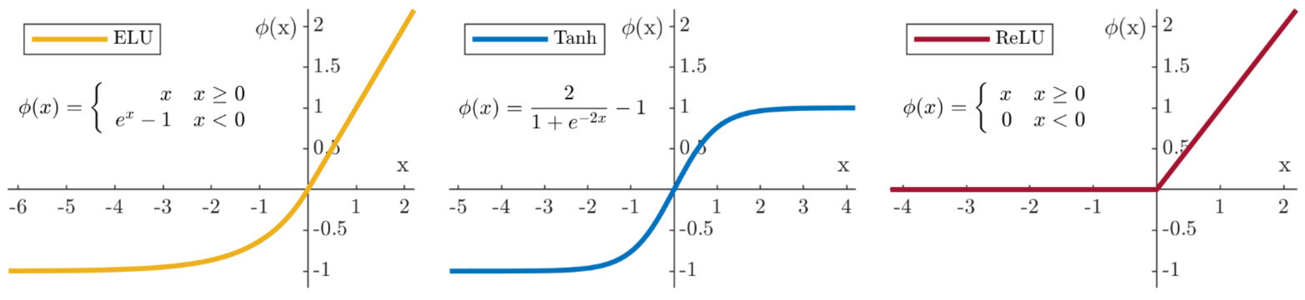
3.1. Artificial Neural Networks

ANNs are nonlinear mathematical models that aim to simulate the human brain processing schemes [56,57,58,59]. In a first approximation, an ANN is the result of the weighted and biased connections of logistic regression units, i.e., the artificial neurons. In a multilayer feedforward network, such neurons are organized into hidden layers between an input layer, consisting of source nodes (the components of the input vector), and an output layer composed of one or more computational neurons that compute the response of the network. Each neuron is characterized by an activation function that limits the range of its response to a continuous value between 0 and 1.

The input, i.e., the feature vector or the hidden layer output, is weighted, meaning that a certain weight is associated to each input signal (the components of the input feature vector or the hidden neurons’ individual responses). These network parameters are learned through a supervised training process so that the network itself (at this point interpretable as a nonlinear parametric function) can perform a specific task. In regression problems, the network’s task is to predict the experimental target associated with a given feature vector, i.e., to represent the implicit relationship between the input and the ground-truth output.

In formal terms, given a data set of input–output vector pairs:

$$D={\left\{\left({\mathit{x}}_{ }{}^{\left(d\right)} ,{\mathit{y}}_{ }{}^{\left(d\right)}\right)\right\}}^{\left|D\right|}{}_{d=1}$$

(1)

$$\mathrm{where} {\mathit{x}}^{\left(d\right)}=\left[x^{\left(d\right)}{}_0,\dots ,x^{\left(d\right)}{}_{F-1}\right]\in R^F \mathrm{and} y^{\left(d\right)}=\left[{\mathit{y}}^{\left(d\right)}{}_0,\dots , y^{\left(d\right)}{}_T\right] \in R^T$$

(2)

and the input layer of an ANN is referred as being the input feature vector ${\mathit{x}}^{\left(d\right)}$. The first hidden layer’s output is the vector:

$${\mathit{h}}^{\left(1\right)}=\left[h_0^{\left(1\right)},\dots ,h_{N-1}^{\left(1\right)}\right]$$

(3)

where each item $h_j^{\left(1\right)}$ is obtained as:

$$h_j^{\left(1\right)}=\varphi \left({{\displaystyle \sum }}_{i=0}^{F-1}{w}_{ij}^{\left(1\right)}·x_i+b_j^{\left(1\right)}\right).$$

(4)

In this expression, $w_{ij}^{\left(1\right)}$ are the weights of the connections between the neurons $x^{\left(d\right)}{}_i$ and the neurons $h_j^{\left(1\right)}$, $b_j^{\left(1\right)}$ are the biases and $\varphi$ is the activation function. The subsequent layer, ${\mathit{h}}^{\left(2\right)}$, is computed in a similar way, by considering the items of the vector ${\mathit{h}}^{\left(1\right)}$ as input layer, with corresponding weights $w_{ij}^{\left(2\right)}$ and biases $b_j^{\left(2\right)}$:

$$h_j^{\left(2\right)}=\varphi \left({{\displaystyle \sum }}_{i=0}^{N-1}{w}_{ij}^{\left(2\right)}·h_i^{\left(1\right)}+b_j^{\left(2\right)}\right).$$

(5)

This process is repeated to compute the activations of each layer ${\mathit{h}}^{\left(l\right)},l\in \left\{1,2,\dots ,L\right\}$ and the output $\widehat{{\mathit{y}}^{\left(d\right)}}={\varphi }^{\left(out\right)}\left({\mathit{h}}^{\left(L\right)}\right)$. All the learnable parameters are considered to form the set:

$$W=\{w_{ij}^{\left(l\right)},b_j^{\left(l\right)} | l \in \left\{1,2,\dots ,L\right\}\}.$$

(6)

In the proposed ANN: the number of source nodes is equal to the number of input features (F = 3), namely, the bitumen content (BC), the filler-to-bitumen ratio (FtB), along with a categorical variable that distinguishes the bituminous mixture in terms of bitumen type, maximum nominal grain size, aggregate type, and production site (values: 1 for M1, 2 for M2, 3 for M3 and so on). These features are fundamental parameters of the pavement engineering, related to the composition of the bituminous mixtures.

Each hidden layer is equipped with N neurons and passed to $\varphi \left(·\right)$ being either an ELU, TanH or ReLU function (Figure 5). The output layer consists of $T=4$ neurons (corresponding to MS, MF, ITSM, and AV) and the identity activation function is considered ${\varphi }^{\left(out\right)}\left(.\right)$. In previous studies, Marshall parameters, as well as ITSM, rather than volumetric properties, have been always determined separately, by means of different neural models [29,45,46,47,48,55], while in the current paper they can be predicted simultaneously by a single multi-output ANN model.

3.2. ANN Optimization

The network parameters $W$ are identified by means of a supervised training process, which is divided into two successive steps, i.e., a forward and a backward phase. In the latter, a backpropagation algorithm [58] is exploited to update the ANN’s weight and biases:

$$W^{\left(e\right)}=W^{\left(e-1\right)}-\alpha \nabla E\left[W^{\left(e-1\right)}\right],e\in \left\{0,\dots ,E-1\right\}$$

(7)

where $E$ is the number of training iterations, $\alpha$ is the learning rate and $W^{\left(e-1\right)}$ are the parameters values at iteration $e-1$. A detailed and comprehensive description of the Equation (7) has already been widely discussed, e.g., by Baldo et al. [29]. At the end of the training process (i.e., after the $\mathrm{E}$ iterations have been completed), the parameters $W$ of the e-th iteration that produced the minimum of the loss function $L$ are selected. Such loss function is usually defined as the 2-norm of the difference between the network output $\widehat{{\mathit{y}}^{\left(d\right)}}$ and the ground-truth vector ${\mathit{y}}^{\left(d\right)},$ thus being called Mean Squared Error (MSE):

$$L\left(\widehat{{\mathit{y}}^{\left(d\right)}},{\mathit{y}}^{\left(d\right)}\right)=\parallel \widehat{{\mathit{y}}^{\left(d\right)}}-{\mathit{y}}^{\left(d\right)}{\parallel }_2^2$$

(8)

The training process just outlined is known as Stochastic Gradient Descent (SGD). Such approach is commonly used in the well-known [60,61] and widely used MATLAB^® ANN Toolbox [22,23,29,45,46,50].

With the aim of increasing the convergence speed of the learning algorithm, several improvements have been proposed in recent years. The first remarkable one, called RAdam optimizer [62], faces the issue of implementing warmup heuristics to avoid falling in bad local minima. This problem can occur using adaptive optimizers such as Adam [63]. According to the authors, the variance of the adaptive learning rate in the initial weight updates can be intractable and direct the solution search towards local minima with poor performance. Adding a rectifier operation to the adaptive learning rate was shown to reduce the variance and lead to better solutions. The second remarkable improvement, Lookahead [64], is a suitable method in reducing the need for extensive hyperparameters search, and the variance of the parameter updates. The Lookahead algorithm maintains two copies of the parameters, respectively, the “fast weights” and “slow weights”. The first is initially updated for k times using a standard SGD-based optimizer. Then, the second set of weights is updated in the direction (i.e., the gradient) of the last computed fast weights. Intuitively, as the name states, the first kind of update looks ahead to acquire information of the loss function’s surface. Once obtained, the gradients used for the actual weight update result in a more accurate direction towards the loss function’s minimum. The combination of the strategies is known as Ranger optimizer. In this work, such optimization algorithm was used to calculate the optimal weights of the implemented ANN, in contrast with the common procedures of neural modeling used in previous literature studies [22,23,29,31,45,46,50].

3.3. ANN Regularization

To perform proper neural modeling, the overfitting phenomenon must be avoided: a model becomes overfitted when it starts to excessively adapt to the training data and stops smoothly regressing the selected validation data. In the current study setup, the weight decay technique [65] (also known as L2 Regularization) has been implemented to overcome such problem. It consists in adding an additional term to the optimization objective, which is calculated as the 2-norm of the parameters of the network. In this way, the global optimization objective becomes:

$$L_{ opt}\left(\widehat{{\mathit{y}}^{\left(d\right)}},{\mathit{y}}^{\left(d\right)},W^{\left(e-1\right)}\right)=L\left(\widehat{{\mathit{y}}^{\left(d\right)}},{\mathit{y}}^{\left(d\right)}\right)+\beta \parallel W^{\left(e-1\right)}{\parallel }_2^2$$

(9)

where $\beta$ is a hyperparameter to control the magnitude of the term.

3.4. k-Fold Cross Validation

A fixed training–validation split of data is usually performed [60,61]: this technique, also known as a “hold-out” method, can result in biased model performance as a consequence of the different descriptive statistics characterizing training and validation data sets [49].

Conversely, the k-fold Cross Validation (k-fold CV) represents an effective alternative to evaluate the actual model generalization capabilities. This resampling method suggests splitting the data set of interest into k folds, equally sized. For example, in the current study setup, a 5-fold CV was implemented. It means that 5 alternative partitions of the data set were obtained: in turn, 4 folds were used to train the neural model and the remaining one to validate it. This involved running 5 experiments, at the end of which the obtained validation scores were averaged to evaluate the general performance capabilities of the proposed model [49,51].

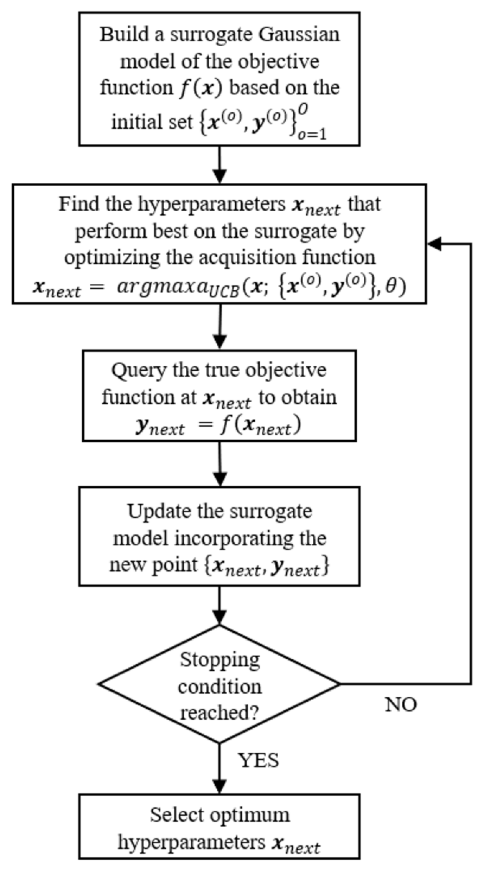
3.5. Bayesian Hyperparameters Optimization

Modeling by machine learning (ML) approaches involves the accurate setting of several hyperparameters: these parameters are used to define the topology and size of a neural network (e.g., the number of hidden layers and neurons), and to control the learning process (e.g., the learning rate). Standard procedures involve a grid or random (i.e., based on a sampling method) search for the best combination of hyperparameters within variation intervals accurately defined by the experimenter on the basis of his/her experience [23,29,31,45,46,48,50]. However, to obviate the significant time demands and computational resources of the abovementioned methods, a semi-automatic strategy has been implemented in the current study, namely, the Bayesian Optimization (BO). This method, based on Bayesian statistics, aims to find the maximum (for maximization problems) or the minimum (for minimization problems) of a function: $f\left(\mathit{x}\right), \mathit{x}=\left[x_p\right], p\in \left\{0,\dots ,P\right\}, P\in N$, where $x_p$ is a parameter in a bounded set $X_p\subset R$. This mathematical problem is solved by optimization algorithms that define a probabilistic model over $f\left(x\right)$, to decide at each iteration which is the most likely point in $X$ to maximize (or minimize) $f\left(·\right)$. In this context, Snoek et al. [66] were the first to use the BO for the search of ML model hyperparameters: since the trend of the objective function is unknown, the authors treated $f\left(·\right)$ as a random function and placed a Gaussian process (GP) prior [67] over it, to capture its behavior. During the optimization process, the prior is updated based on ML experiments results, produced by different hyperparameters combinations, to form the posterior distribution over the function $f\left(·\right)$. The latter, in turn, is exploited by an acquisition function to determine the next evaluation point.

In practice (Figure 6), a set of $O$ observations of the form ${\left\{{\mathit{x}}^{\left(o\right)}, {\mathit{y}}^{\left(o\right)}\right\}}_{o=1}^O$, with ${\mathit{y}}^{\left(o\right)}=N\left(f\left({\mathit{x}}^{\left(o\right)}\right), \nu \right)$ and where $\nu$ is the variance of noise in the observation of $f\left(·\right)$, is exploited to determine a multivariate Gaussian distribution over $R^O$ through a mean $m: X\to R$ and covariance $K: X\times X\to R$ functions. The next set of hyperparameters ${\mathit{x}}_{next}\in X$ that should be evaluated during the optimization process is determined by solving the equation ${\mathit{x}}_{next}=argma{x}_{\mathit{x}}a\left(\mathit{x}\right)$. The function $a: X\to R^{+}$ is called acquisition function and generally depends on both the previously observed samples ${\left\{{\mathit{x}}^{\left(o\right)}, {\mathit{y}}^{\left(o\right)}\right\}}_{o=1}^O$ and the GP parameters $\theta$. It is formulated as follows: $a\left(\mathit{x};\left\{{\mathit{x}}^{\left(o\right)}, {\mathit{y}}^{\left(o\right)}\right\},\theta \right)$. In the GP prior setting, $a\left(·\right)$ relies on the predictive mean $\mu \left(\mathit{x}; \left\{{\mathit{x}}^{\left(o\right)}, {\mathit{y}}^{\left(o\right)}\right\}, \theta \right)$ and variance ${\sigma }^2\left(\mathit{x}; \left\{{\mathit{x}}^{\left(o\right)}, {\mathit{y}}^{\left(o\right)}\right\}, \theta \right)$ functions of the GP model. There are several existing definitions for $a\left(·\right)$ [68,69], but the GP Upper Confidence Bound (UCB) [70] has been proven to efficiently reduce the number of function evaluations needed to determine the global optimum of several black-box multimodal functions. UCB implements the acquisition function as $a_{UCB}\left(\mathit{x}; \left\{{\mathit{x}}^{\left(o\right)}, {\mathit{y}}^{\left(o\right)}\right\},\theta \right)=\mu \left(\mathit{x}; \left\{{\mathit{x}}^{\left(o\right)}, {\mathit{y}}^{\left(o\right)}\right\}, \theta \right)-\kappa \sigma \left(\mathit{x}; \left\{{\mathit{x}}^{\left(o\right)}, {\mathit{y}}^{\left(o\right)}\right\}, \theta \right)$, where $\kappa$ is a hyperparameter to control the balance between exploitation (i.e., favoring parts that the model predicts as promising) and exploration.

In the actual problem, namely the prediction of mechanical and volumetric properties of bituminous mixtures for road pavement, $f\left(·\right)$ is defined as $f:X_L\times X_N\times X_{act}\times X_{\alpha }\times X_{\beta }\times X_E\to \left[-1,1\right]$ and has to be maximized. Therefore, given the $P=6$ hyperparameters $L,N,act,\alpha ,\beta ,E$, $f\left(·\right)$ constructs an ANN with L layers, N neurons per layer and performs a 5-fold CV experiment in which the ANN is trained for E iterations with $\alpha$ and $\beta$ as the learning rate and weight decay parameter, respectively. $f\left(·\right)$ returns a scalar value that expresses the average Pearson coefficient (R) obtained by the ANN on the 5 validation folds. The BO algorithm performs 500 iterations: at each iteration, $f\left(·\right)$ runs an experiment based on the hyperparameter combination sampled by the UCB algorithm on the posterior distribution; the result is used to update such probabilistic model and improve sampling of next points. The step-by-step procedure is described in Figure 7: the modeling procedure begins with the mixtures design and the execution of laboratory tests for the definition of features and targets variables; these latter are assumed to be representative of the physical problem treated; the input-target fitting is performed by a neural network, whose structure and algorithmic functioning is not known a priori; the search for the topology and the values of the training process parameters that minimize the prediction error of the ANN is handled by the Bayesian optimizer, by comparing network outputs and experimental targets; once the optimal hyperparameters combination has been identified, the model can be put into service for the designed application, by training it on the entire data set. In the current study setup, the hyperparameters to be optimized by the Bayesian approach can range in the following integer or logarithmic intervals:

• $X_L=\left\{1,\dots ,5\right\}$, for the number of hidden network layers L;
• $X_N=\left\{4,\dots ,64\right\}$, for the number of neurons $N$ for each hidden layer;
• $X_{act}=\left\{tanh,ReLU,ELU\right\}$ for the set of activation functions to be applied after each hidden layer;
• $X_{\alpha }=\left[{10}^{-6},{10}^{-2}\right]$ for the learning rate $\alpha$;
• $X_{\beta }=\left[{10}^{-6},{10}^{-2}\right]$ for the weight decay parameter $\beta$;
• $X_E=\left\{500,\dots ,5000\right\}$ for the number of learning process iterations.

These ranges were defined in the optimizer implementation [67] and have been left unchanged.

3.6. Implementation Details

Before being inputted to the ANN, each feature contained in the feature vectors ${\mathit{x}}^{\left(d\right)}$ was standardized, i.e., the respective mean was subtracted and division by the respective standard deviation was applied. The statistics were calculated on $D$. The same procedure was performed for the target feature vectors ${\mathit{y}}^{\left(d\right)}$, where each target variable was subtracted by its mean and divided by its standard deviation computed on $D$. Also, the BO observations ${\mathit{x}}^{\left(o\right)}$ were transformed in a similar fashion. In this case, each hyperparameter was standardized by the mean and standard deviation of the respective range.

The source code was written with the Python language. ANNs were implemented using the PyTorch machine learning framework, while the hyperparameters BO procedure was realized with the Bayesian optimization package [71]. The code was run on a machine provided with an Intel(R) Xeon(R) W-2125 4GHz CPU and 32GB of RAM running Ubuntu 18.04. Each experiment lasted circa 24 h.

4. Results and Discussion

Figure 8 shows the k-fold CV score of neural models that were designed in the 500 iterations of the BO algorithm. The Pearson’s R coefficient averaged over the 5 validation folds tended to become uniform in value among the different combinations tested by the BO optimizer at least during the first 350 iterations (Figure 8) but showed more marked variations afterwards. The algorithm has detected a region of the search space where the validation error was not significantly changing and, having assessed an over-exploration of a specific zone, it has decided to focus its search on an unexplored area that might have high-performing solutions (however, identifying worse combinations). This result highlights the regulation between exploitation and exploration performed by the UCB algorithm.

Despite the large size of the search space, the optimal model (i.e., showing the minimum validation loss MSE_CV = 0.249 and then the maximum value of the Pearson coefficient R_CV = 0.868) was found at iteration 54 (Figure 8). The hyperparameters discovered by the BO algorithm defined an ANN with $L$ = 5 layers, $N$ = 37 neurons, and hyperbolic tangent activation function ($tanh$), that was trained for $E$ = 3552 iterations, with a learning rate of $\alpha$ = 0.01 and weight decay $\beta$ = $1·{10}^{-6}$.

Table 5. Number and codes of Marshall specimens.

Fold	MSEmean	R—Pearson Correlation Coefficient				Rmean
		ITSM	MS	MF	AV
0	0.219	0.837	0.866	0.842	0.964	0.877
1	0.203	0.963	0.835	0.725	0.973	0.874
2	0.254	0.872	0.836	0.799	0.917	0.856
3	0.223	0.918	0.826	0.917	0.956	0.905
4	0.346	0.841	0.731	0.834	0.912	0.829
CVresult	0.249	0.886	0.819	0.824	0.944	0.868

shows the validation MSE (second column) and the R-score of the optimal model for each of the 5 folds (last column). In addition, the final average results for each mechanical characteristic and volumetric property are reported in the last row of Table 5. Figure 9 shows the relation between network output and experimental target for each fold.

Although there is a high variability in the data set, which can be explained by considering the different properties of the mixtures analysed, the optimal BO model returns very successful results (Figure 9). The 5-folds averaged Pearson coefficient for each mechanical and physical parameter is always greater than 0.819 (last row of Table 5). Fluctuations in values of the MSE and R parameters (second and seventh column in Table 5) can be attributed to the different distribution of training and test data that characterize each fold. This result shows how a fixed split of the data set can lead to an incorrect assessment of the prediction error, which can be worse (R₄ = 0.829) or better (R₃ = 0.906) than the most likely situation represented by the k-fold CV (R_CV = 0.868). Random and grid searches based on the prediction error by a fixed split training test may find solutions that are not optimal [49], due to fluctuations resulting from considering one partition rather than another. Figure 10 shows the comparison between experimental targets and predicted outputs, for the four parameters analyzed, as regards fold 4. Values calculated by the ANN model characterized by the highest prediction error (MSE_mean = 0.346, Table 5) are very close in value to the experimental data, whatever variable is considered. This result is relevant from an engineering point of view, because it proves that ANNs can be an accurate method to model (even simultaneously) the mechanical response and physical properties of bituminous mixtures, also very different in terms of composition.

Although the presented modeling procedure is conceptually and computationally more complex than a simple grid search, it overcomes some of the problems (such as biased performance evaluations and sub-optimal hyperparameters selection) inherent in traditional methods (i.e., grid and random search) or in the most frequently used toolboxes (such as the MATLAB^® ANN Toolbox), as the above reported results suggest.

5. Conclusions

The main goal of this study was to present and discuss a semi-automatic and unbiased procedure to select the most reliable ANN model for a given predictive modeling problem, which can overcome the limitations of conventional approaches. In particular, the focus was on predicting at once volumetric properties and mechanical characteristics of bituminous mixtures prepared using different types of bitumen and aggregate, binder content and maximum nominal grain size, to support the mix design phase, providing numerical estimations of the investigated parameters without any other costly laboratory test. The study results can be summarized as follows:

• To perform proper neural modeling, the evaluation of the several network structures resulting from the selection of different model hyperparameters values is required. The procedure developed in this article allowed the limitations of the most widely used ANN toolbox to be overcome.
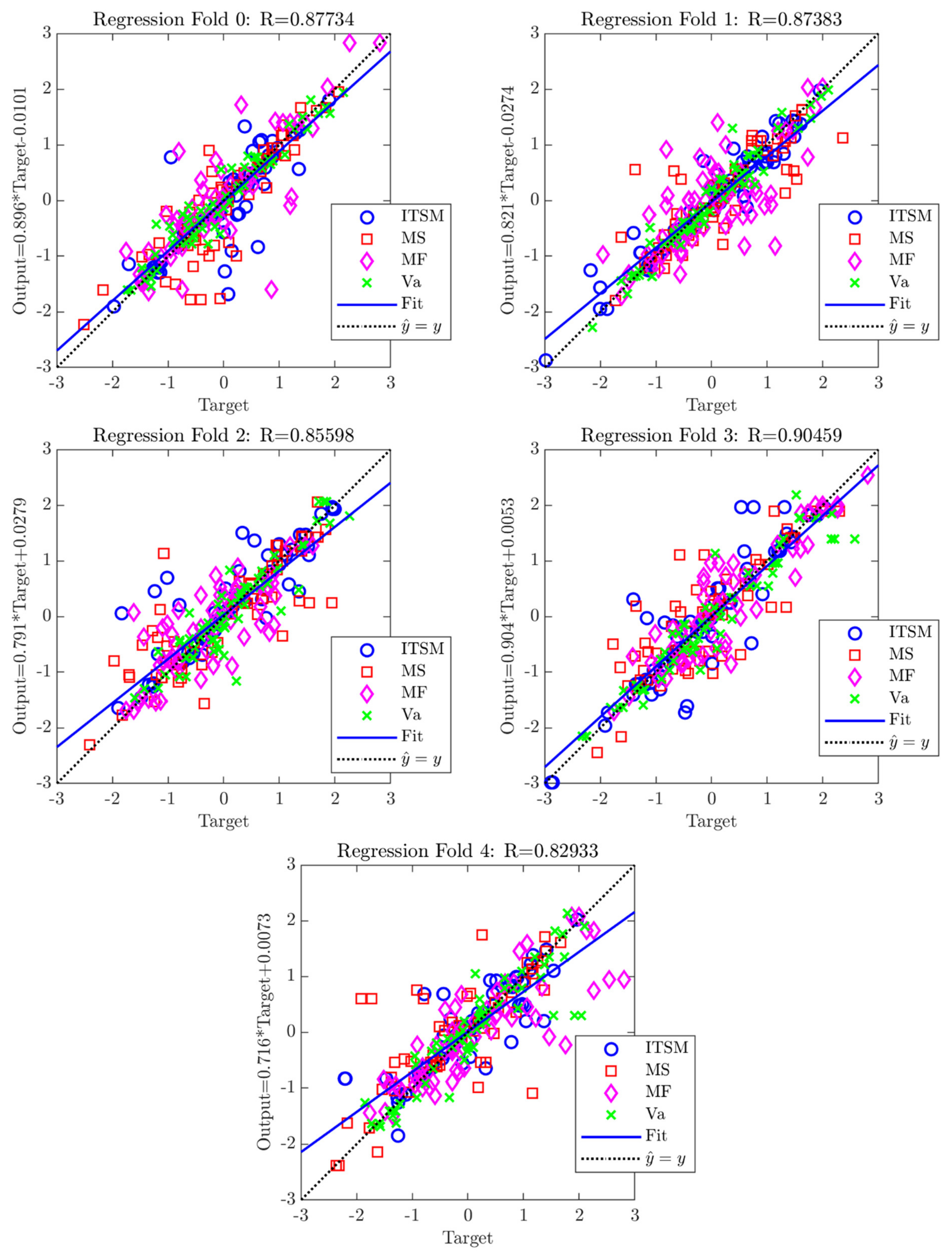
• The proposed approach with the k-fold CV produces more reliable results in terms of model validation error, with respect to the standard grid search based on a random data set partition: in fact, if the procedure were based on a fixed random split of the available data set, different results are possible, worse (R₄ = 0.829) or better (R₃ = 0.906) than the most likely situation represented by the k-fold CV (R_CV = 0.868), due to the different distribution of the training and validation data.
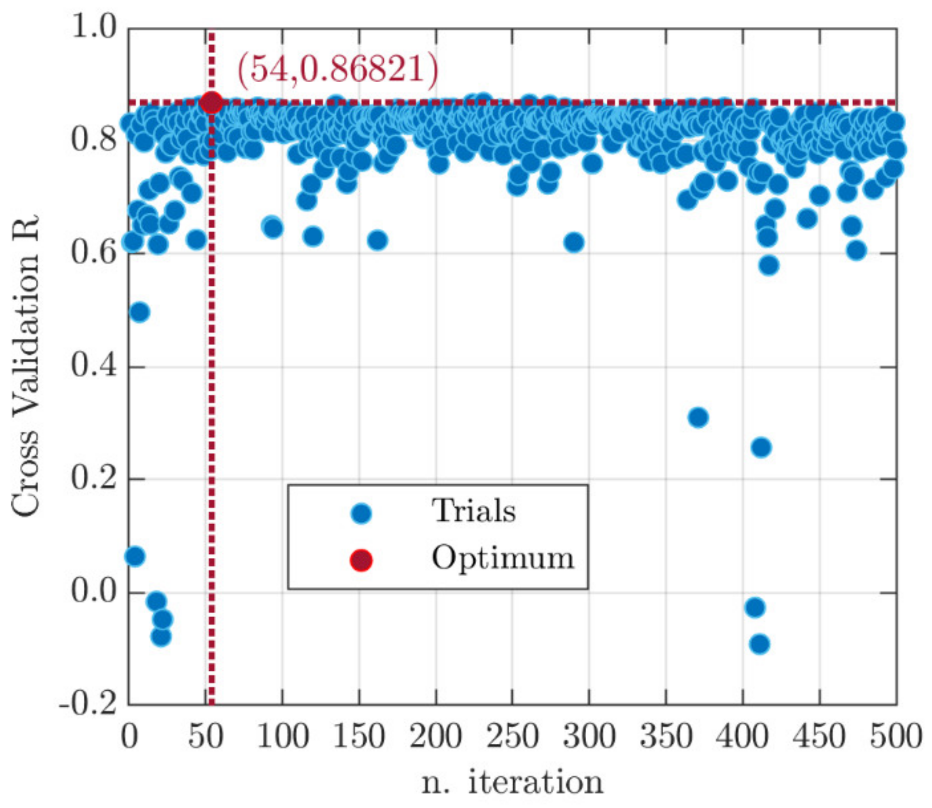
• The BO algorithm has shown to be successful in solving the challenging problem of properly setting the model hyperparameters: it has identified the optimal solution, in terms of algorithmic and structural configuration of the ANN, in only 54 iterations. The hallmark of such a technique lies in the ability to take past evaluations into account so as to limit the loss function recalls. Nonetheless, the reader should be aware that the BO procedure results may be linked to the constraints set by the research engineer in terms of hyperparameters’ variability.
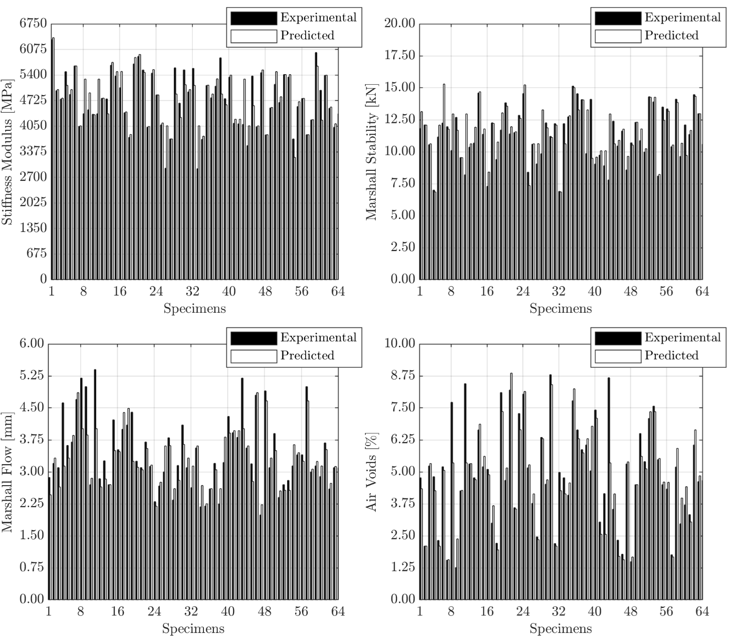
• In the current paper, Marshall parameters, ITSM, as well as AV content have been determined simultaneously by a single multi-output ANN, unlike previous studies; therefore, such approach represents an integrated predictive model of the selected mechanical and volumetric properties.
• The neural network structure best suited (MSE_CV = 0.249, R_CV = 0.868) to model experimental mixtures data is defined by 5 layers, 37 neurons in each hidden layer and $tanh$ transfer function. A learning step size $\alpha$ equal to 0.01 and weight decay $\beta$ equal to $1\times {10}^{-6}$ are implemented in the Ranger training algorithm.
• The algorithms applied and the analytical steps taken by the artificial networks have been illustrated in detail to make the procedure followed replicable to the reader. If it is desired to put the proposed model into service for the designed application (e.g., use in a laboratory or plant for estimates of mechanical parameters and volumetric properties of bituminous mixtures), then the optimized ANN must be trained with all available data.

It is worth recalling that the proposed model is applicable only to the specific types of aggregate, bitumen and mixture structure considered. This study did not account for the influence of different aggregate gradation on the results for a specific bitumen content. An interesting further development would be to investigate such an effect, integrating new input variables related to aggregate gradation or mix proportioning. Alternatively, the modeling variables relating to the mechanical characteristics of the mixture could be replaced by those relating to the road pavement performance, such as fatigue and permanent deformation resistance. This replacement would represent further progress towards a performance-based mix design.

References

1. Zhou, F.; Scullion, T.; Sun, L. Verification and modeling of three-stage permanent deformation behavior of asphalt mixes. J. Transp. Eng. 2004, 130, 486–494. [Google Scholar] [CrossRef]
2. Gandomi, A.H.; Alavi, A.H.; Mirzahosseini, M.R.; Nejad, F.M. Nonlinear genetic-based models for prediction of flow number of asphalt mixtures. J. Mater. Civ. Eng. 2011, 23, 248–263. [Google Scholar] [CrossRef]
3. Alavi, A.H.; Ameri, M.; Gandomi, A.H.; Mirzahosseini, M.R. Formulation of flow number of asphalt mixes using a hybrid computational method. Constr. Build. Mater. 2011, 25, 1338–1355. [Google Scholar] [CrossRef]
4. Dias, J.L.F.; Picado-Santos, L.; Capitão, S. Mechanical performance of dry process fine crumb rubber asphalt mixtures placed on the Portuguese road network. Constr. Build. Mater. 2014, 73, 247–254. [Google Scholar] [CrossRef]
5. Liu, Q.T.; Wu, S.P. Effects of steel wool distribution on properties of porous asphalt concrete. Key engineering materials. Trans. Tech Publ. 2014, 599, 150–154. [Google Scholar] [CrossRef]
6. Garcia, A.; Norambuena-Contreras, J.; Bueno, M.; Partl, M.N. Influence of steel wool fibers on the mechanical, termal, and healing properties of dense asphalt concrete. J. Test. Eval. 2014, 42, 1107–1118. [Google Scholar] [CrossRef]
7. Pasandín, A.; Pérez, I. Overview of bituminous mixtures made with recycled concrete aggregates. Constr. Build. Mater. 2015, 74, 151–161. [Google Scholar] [CrossRef] [Green Version]
8. Zaumanis, M.; Mallick, R.B.; Frank, R. 100% hot mix asphalt recycling: Challenges and benefits. Transp. Res. Procedia 2016, 14, 3493–3502. [Google Scholar] [CrossRef] [Green Version]
9. Wang, L.; Gong, H.; Hou, Y.; Shu, X.; Huang, B. Advances in pavement materials, design, characterisation, and simulation. Road Mater. Pavement Des. 2017, 18, 1–11. [Google Scholar] [CrossRef]
10. Erkens, S.; Liu, X.; Scarpas, A. 3D finite element model for asphalt concrete response simulation. Int. J. Geomech. 2002, 2, 305–330. [Google Scholar] [CrossRef]
11. Giunta, M.; Pisano, A.A. One-dimensional visco-elastoplastic constitutive model for asphalt concrete. Multidiscip. Modeling Mater. Struct. 2006, 2, 247–264. [Google Scholar] [CrossRef]
12. Underwood, S.B.; Kim, R.Y. Viscoelastoplastic continuum damage model for asphalt concrete in tension. J. Eng. Mech. 2011, 137, 732–739. [Google Scholar] [CrossRef]
13. Yun, T.; Kim, Y.R. Viscoelastoplastic modeling of the behavior of hot mix asphalt in compression. KSCE J. Civ. Eng. 2013, 17, 1323–1332. [Google Scholar] [CrossRef]
14. Pasetto, M.; Baldo, N. Computational analysis of the creep behaviour of bituminous mixtures. Constr. Build. Mater. 2015, 94, 784–790. [Google Scholar] [CrossRef]
15. Di Benedetto, H.; Sauzéat, C.; Clec’h, P. Anisotropy of bituminous mixture in the linear viscoelastic domain. Mech. Time Depend. Mater. 2016, 20, 281–297. [Google Scholar] [CrossRef]
16. Pasetto, M.; Baldo, N. Numerical visco-elastoplastic constitutive modelization of creep recovery tests on hot mix asphalt. J. Traffic Transp. Eng. 2016, 3, 390–397. [Google Scholar] [CrossRef]
17. Darabi, M.K.; Huang, C.W.; Bazzaz, M.; Masad, E.A.; Little, D.N. Characterization and validation of the nonlinear viscoelastic- viscoplastic with hardening-relaxation constitutive relationship for asphalt mixtures. Constr. Build. Mater. 2019, 216, 648–660. [Google Scholar] [CrossRef]
18. Kim, S.H.; Kim, N. Development of performance prediction models in flexible pavement using regression analysis method. KSCE J. Civ. Eng. 2006, 10, 91–96. [Google Scholar] [CrossRef]
19. Laurinavičius, A.; Oginskas, R. Experimental research on the development of rutting in asphalt concrete pavements reinforced with geosynthetic materials. J. Civ. Eng. Manag. 2006, 12, 311–317. [Google Scholar] [CrossRef]
20. Shukla, P.K.; Das, A. A re-visit to the development of fatigue and rutting equations used for asphalt pavement design. Int. J. Pavement Eng. 2008, 9, 355–364. [Google Scholar] [CrossRef]
21. Rahman, A.A.; Mendez Larrain, M.M.; Tarefder, R.A. Development of a nonlinear rutting model for asphalt concrete based on Weibull parameters. Int. J. Pavement Eng. 2019, 20, 1055–1064. [Google Scholar] [CrossRef]
22. Specht, L.P.; Khatchatourian, O.; Brito, L.A.T.; Ceratti, J.A.P. Modeling of asphalt-rubber rotational viscosity by statistical analysis and neural networks. Mater. Res. 2007, 10, 69–74. [Google Scholar] [CrossRef]
23. Mirzahosseini, M.R.; Aghaeifar, A.; Alavi, A.H.; Gandomi, A.H.; Seyednour, R. Permanent deformation analysis of asphalt mixtures using soft computing techniques. Expert Syst. Appl. 2011, 38, 6081–6100. [Google Scholar] [CrossRef]
24. Androjić, I.; Marović, I. Development of artificial neural network and multiple linear regression models in the prediction process of the hot mix asphalt properties. Can. J. Civ. Eng. 2017, 44, 994–1004. [Google Scholar] [CrossRef]
25. Alrashydah, E.I.; Abo-Qudais, S.A. Modeling of creep compliance behavior in asphalt mixes using multiple regression and artificial neural networks. Constr. Build. Mater. 2018, 159, 635–641. [Google Scholar] [CrossRef]
26. Ziari, H.; Amini, A.; Goli, A.; Mirzaiyan, D. Predicting rutting performance of carbon nano tube (CNT) asphalt binders using regression models and neural networks. Constr. Build. Mater. 2018, 160, 415–426. [Google Scholar] [CrossRef]
27. Montoya, M.A.; Haddock, J.E. Estimating asphalt mixture volumetric properties using seemingly unrelated regression equations approaches. Constr. Build. Mater. 2019, 225, 829–837. [Google Scholar] [CrossRef]
28. Lam, N.-T.-M.; Nguyen, D.-L.; Le, D.-H. Predicting compressive strength of roller-compacted concrete pavement containing steel slag aggregate and fly ash. Int. J. Pavement Eng. 2020, 2020, 1–14. [Google Scholar] [CrossRef]
29. Baldo, N.; Manthos, E.; Pasetto, M. Analysis of the mechanical behaviour of asphalt concretes using artificial neural networks. Adv. Civ. Eng. 2018, 2018, 1650945. [Google Scholar] [CrossRef] [Green Version]
30. Tarefder, R.A.; White, L.; Zaman, M. Neural network model for asphalt concrete permeability. J. Mater. Civ. Eng. 2005, 17, 19–27. [Google Scholar] [CrossRef]
31. Ozsahin, T.S.; Oruc, S. Neural network model for resilient modulus of emulsified asphalt mixtures. Constr. Build. Mater. 2008, 22, 1436–1445. [Google Scholar] [CrossRef]
32. Tapkın, S.; Çevik, A.; Uşar, Ü. Accumulated strain prediction of polypropylene modified marshall specimens in repeated creep test using artificial neural networks. Expert Syst. Appl. 2009, 36, 11186–11197. [Google Scholar] [CrossRef]
33. Xiao, F.; Amirkhanian, S.; Juang, C.H. Prediction of fatigue life of rubberized asphalt concrete mixtures containing reclaimed asphalt pavement using artificial neural networks. J. Mater. Civ. Eng. 2009, 21, 253–261. [Google Scholar] [CrossRef]
34. Ahmed, T.M.; Green, P.L.; Khalid, H.A. Predicting fatigue performance of hot mix asphalt using artificial neural networks. Road Mater. Pavement Des. 2017, 18, 141–154. [Google Scholar] [CrossRef]
35. Ceylan, H.; Schwartz, C.W.; Kim, S.; Gopalakrishnan, K. Accuracy of predictive models for dynamic modulus of hot-mix asphalt. J. Mater. Civ. Eng. 2009, 21, 286–293. [Google Scholar] [CrossRef] [Green Version]
36. Le, T.-H.; Nguyen, H.-L.; Pham, B.T.; Nguyen, M.H.; Pham, C.-T.; Nguyen, N.-L.; Le, T.-T.; Ly, H.-B. Artificial intelligence-based model for the prediction of dynamic modulus of stone mastic asphalt. Appl. Sci. 2020, 10, 5242. [Google Scholar] [CrossRef]
37. Ghorbani, B.; Arulrajah, A.; Narsilio, G.; Horpibulsuk, S.; Bo, M.-W. Thermal and mechanical properties of demolition wastes in geothermal pavements by experimental and machine learning techniques. Constr. Build. Mater. 2021, 280, 122499. [Google Scholar] [CrossRef]
38. Aksoy, A.; Iskender, E.; Kahraman, H.T. Application of the intuitive k-NN Estimator for prediction of the Marshall Test (ASTM D1559) results for asphalt mixtures. Constr. Build. Mater. 2012, 34, 561–569. [Google Scholar] [CrossRef]
39. Van Thanh, D.; Feng, C.P. Study on marshall and rutting test of SMA at abnormally high temperature. Constr. Build. Mater. 2013, 47, 1337–1341. [Google Scholar] [CrossRef]
40. Abdoli, M.; Fathollahi, A.; Babaei, R. The application of recycled aggregates of construction debris in asphalt concrete mix design. Int. J. Environ. Res. 2015, 9, 489–494. [Google Scholar] [CrossRef]
41. Sarkar, D.; Pal, M.; Sarkar, A.K.; Mishra, U. Evaluation of the properties of bituminous concrete prepared from brick-stone mix aggregate. Adv. Mater. Sci. Eng. 2016, 2016, 2761038. [Google Scholar] [CrossRef] [Green Version]
42. Xu, B.; Chen, J.; Zhou, C.; Wang, W. Study on Marshall design parameters of porous asphalt mixture using limestone as coarse aggregate. Constr. Build. Mater. 2016, 124, 846–854. [Google Scholar] [CrossRef]
43. Zumrawi, M.M.; Khalill, F.O. Experimental study of steel slag used as aggregate in asphalt mixture. Am. J. Constr. Build. Mater. 2017, 2, 26–32. [Google Scholar] [CrossRef]
44. Al-Ammari, M.A.S.; Jakarni, F.M.; Muniandy, R.; Hassim, S. The effect of aggregate and compaction method on the physical properties of hot mix asphalt. IOP Conf. Ser. Mater. Sci. Eng. 2019, 512, 012003. [Google Scholar] [CrossRef]
45. Tapkın, S.; Çevik, A.; Uşar, Ü. Prediction of Marshall test results for polypropylene modified dense bituminous mixtures using neural networks. Expert Syst. Appl. 2010, 37, 4660–4670. [Google Scholar] [CrossRef]
46. Ozgan, E. Artificial neural network based modelling of the Marshall Stability of asphalt concrete. Expert Syst. Appl. 2011, 38, 6025–6030. [Google Scholar] [CrossRef]
47. Khuntia, S.; Das, A.K.; Mohanty, M.; Panda, M. Prediction of marshall parameters of modified bituminous mixtures using artificial intelligence techniques. Int. J. Transp. Sci. Technol. 2014, 3, 211–227. [Google Scholar] [CrossRef] [Green Version]
48. Zavrtanik, N.; Prosen, J.; Tušar, M.; Turk, G. The use of artificial neural networks for modeling air void content in aggregate mixture. Autom. Constr. 2016, 63, 155–161. [Google Scholar] [CrossRef]
49. James, G.; Witten, D.; Hastie, T.; Tibshirani, R. Resampling methods. In An Introduction to Statistical Learning; Springer: Berlin/Heidelberg, Germany, 2013; Volume 112, Chapter 5; pp. 176–186. [Google Scholar]
50. Baldo, N.; Manthos, E.; Miani, M. Stiffness modulus and marshall parameters of hot mix asphalts: Laboratory data modeling by artificial neural networks characterized by cross-validation. Appl. Sci. 2019, 9, 3502. [Google Scholar] [CrossRef] [Green Version]
51. Baldo, N.; Miani, M.; Rondinella, F.; Celauro, C. A machine learning approach to determine airport asphalt concrete layer moduli using heavy weight deflectometer data. Sustainability 2021, 13, 8831. [Google Scholar] [CrossRef]
52. Shahriari, B.; Swersky, K.; Wang, Z.; Adams, R.P.; de Freitas, N. Taking the human out of the loop: A review of Bayesian optimization. Proc. IEEE 2015, 104, 148–175. [Google Scholar] [CrossRef] [Green Version]
53. Bergstra, J.; Bardenet, R.; Bengio, Y.; Kégl, B. Algorithms for hyper-parameter optimization. Proceeding of the 24th Advances in Neural Information Processing Systems (NIPS 2011), Granada, Spain, 12–17 December 2011; Shawe-Taylor, J., Zemel, R., Bartlett, P., Pereira, F., Weinberger, K.Q., Eds.; Curran Associates, Inc.: New York, NY, USA, 2011. [Google Scholar]
54. Bergstra, J.; Yamins, D.; Cox, D. Making a science of model search: Hyperparameter optimization in hundreds of dimensions for vision architectures. Int. Conf. Mach. Learn. PMLR 2013, 28, 115–123. [Google Scholar]
55. Xiao, F.; Amirkhanian, S.N. Artificial neural network approach to estimating stiffness behavior of rubberized asphalt concrete containing reclaimed asphalt pavement. J. Transp. Eng. 2009, 135, 580–589. [Google Scholar] [CrossRef]
56. Widrow, B.; Hoff, M.E. Adaptive Switching Circuits; Technical Report; Stanford University, Ca Stanford Electronics Labs: Stanford, CA, USA, 1960. [Google Scholar]
57. Rosenblatt, F. Principles of Neurodynamics: Perceptrons and the Theory of Brain Mechanisms; Technical Report; Cornell Aeronautical Lab Inc.: Buffalo, NY, USA, 1961. [Google Scholar]
58. Rumelhart, D.E.; Hinton, G.E.; Williams, R.J. Learning representations by back-propagating errors. Nature 1986, 323, 533–536. [Google Scholar] [CrossRef]
59. McCulloch, W.S.; Pitts, W. A logical calculus of the ideas immanent in nervous activity. Bull. Math. Biophys. 1943, 5, 115–133. [Google Scholar] [CrossRef]
60. Demuth, H.B.; Beale, M.H.; de Jess, O.; Hagan, M.T. Neural Network Design; Martin Hagan: Stillwater, OK, USA, 2014. [Google Scholar]
61. Hagan, M.T.; Menhaj, M.B. Training feedforward networks with the Marquardt algorithm. IEEE Trans. Neural Netw. 1994, 5, 989–993. [Google Scholar] [CrossRef] [PubMed]
62. Liu, L.; Jiang, H.; He, P.; Chen, W.; Liu, X.; Gao, J.; Han, J. On the variance of the adaptive learning rate and beyond. arXiv 2019, arXiv:1908.03265. [Google Scholar]
63. Kingma, D.P.; Ba, J. Adam: A method for stochastic optimization. arXiv 2014, arXiv:1412.6980. [Google Scholar]
64. Zhang, M.R.; Lucas, J.; Hinton, G.; Ba, J. Lookahead optimizer: K steps forward, 1 step back. arXiv 2019, arXiv:1907.08610. [Google Scholar]
65. Ng, A.Y. Feature selection, L 1 vs. L 2 regularization, and rotational invariance. In Proceedings of the 21th International Conference on Machine learning, Banff, AB, Canada, 4–8 July 2004; pp. 615–622. [Google Scholar] [CrossRef] [Green Version]
66. Snoek, J.; Larochelle, H.; Adams, R.P. Practical bayesian optimization of machine learning algorithms. arXiv 2012, arXiv:1206.2944. [Google Scholar]
67. Rasmussen, C.E. Gaussian Processes in Machine Learning. Summer School on Machine Learning; Springer: Berlin/Heidelberg, Germany, 2003; pp. 63–71. [Google Scholar]
68. Kushner, H.J. A New Method of locating the maximum point of an arbitrary multipeak curve in the presence of noise. J. Basic Eng. 1964, 86, 97–106. [Google Scholar] [CrossRef]
69. Mockus, J.; Tiesis, V.; Zilinskas, A. The application of Bayesian methods for seeking the extremum. In Towards Global Optimization, 2nd ed.; Dixon, L.C.W., Szego, G.P., Eds.; North Holland Publishing Co.: Amsterdam, The Netherlands, 1978; pp. 117–129. [Google Scholar]
70. Srinivas, N.; Krause, A.; Kakade, S.M.; Seeger, M. Gaussian process optimization in the bandit setting: No regret and experimental design. arXiv 2009, arXiv:0912.3995. [Google Scholar]
71. Nogueira, F. Bayesian Optimization: Open Source Constrained Global Optimization Tool for Python. Available online: https://github.com/fmfn/BayesianOptimization (accessed on 25 November 2021).
Figure 1. Gradation curves of lab-prepared BM12.5.
Applsci 11 11710 g001
Figure 2. Gradation curves of lab-prepared BM20.
Applsci 11 11710 g002
Figure 3. Gradation curves of plant-prepared BM20 (gradations of different production dates).
Applsci 11 11710 g003
Figure 4. ITSM test setup.
Applsci 11 11710 g004
Figure 5. Activation functions: exponential linear (ELU), hyperbolic tangent (TanH), rectified linear (ReLU).
Applsci 11 11710 g005
Figure 6. Flow chart of the optimization process.
Applsci 11 11710 g006
Figure 7. Step-by-step procedure followed in this study: it starts with the mix design (left side) and testing processes (bottom side); these tests define the set of target variables (lower right side); the input-target fitting is performed by a neural network, whose structure and algorithmic functioning are searched by the Bayesian optimizer (upper side) comparing network outputs and experimental targets (right side).
Applsci 11 11710 g007
Figure 8. Average R-score on the 5 validation folds for the 500 algorithm iterations.
Applsci 11 11710 g008
Figure 9. Regression analysis on the 5 folds.
Applsci 11 11710 g009
Figure 10. Experimental vs. predicted data, related to fold 4.
Applsci 11 11710 g010