Article

An Approximation-Based Design Optimization Approach to Eigenfrequency Assignment for Flexible Multibody Systems

1
Faculty of Science and Technology, Free University of Bozen-Bolzano, Piazza Università 5, 39100 Bolzano, Italy
2
Department of Industrial Engineering, University of Padova, Via Venezia 1, 35121 Padova, Italy
*
Author to whom correspondence should be addressed.
Appl. Sci. 2021, 11(23), 11558; https://doi.org/10.3390/app112311558
Submission received: 27 September 2021 / Revised: 16 November 2021 / Accepted: 3 December 2021 / Published: 6 December 2021
(This article belongs to the Special Issue Optimization of Nonlinear Vibration in Mechanical Systems)

Abstract

:
The use of flexible multibody simulation has increased significantly over recent years due to the increasingly lightweight nature of mechanical systems. The prominence of lightweight engineering design in mechanical systems is driven by the desire to require less energy in operation and to reach higher speeds. However, flexible lightweight systems are prone to vibration, which can affect reliability and overall system performance. Whether such issues are critical depends largely on the system eigenfrequencies, which should be correctly assigned by the proper choice of the inertial and elastic properties of the system. In this paper, an eigenfrequency assignment method for flexible multibody systems is proposed. This relies on a parametric modal model which is a Taylor expansion approximation of the eigenfrequencies in the neighborhood of a configuration of choice. Eigenfrequency assignment is recast as a quadratic programming problem which can be solved with low computational effort. The method is validated by assigning the lowest eigenfrequency of a two-bar linkage by properly adding point masses. The obtained results indicate that the proposed method can effectively assign the desired eigenfrequency.

1. Introduction

Multibody systems with lightweight and slender links exhibit excellent performance in terms of high attainable speed and low energy consumption. However, flexibility of the links makes such systems prone to vibration, and consequently, prone to fatigue and poor in-position accuracy. Such issues can be greatly mitigated if the system is designed or modified with appropriate eigenfrequencies through modification of physical parameters [1].
From the mathematical point of view, a problem in which a system is designed for specific eigenfrequencies can be regarded as an inverse eigenvalue problem [2], in contrast to the direct eigenvalue problem, in which the eigenfrequencies of a vibrating system are computed. For linear time-invariant systems, the latter has been extensively studied, and the state-of-the-art can be considered very well developed [3]. The task of computing or measuring the eigenfrequencies of a system is often referred to as modal analysis. The inverse problem, which aims at finding a feasible system model from prescribed eigenfrequencies, is ill-posed and therefore intrinsically more challenging. The significance of the inverse problem in engineering (not limited to vibrations) has stimulated fertile research over the past few decades, e.g., [4,5,6,7].
For a flexible-link multibody system (FLMS), linear models are satisfactory only in the proximity of an equilibrium configuration. If large displacements and/or rotations of the links are considered, a nonlinear model is essential in order to account for the dependence on the multibody system configuration. Some of the FLMS modeling techniques available in the literature represent the system dynamics by means of a minimum set of second-order ordinary differential equations, which allow for a straightforward application of modal analysis [8]. One such flexible multibody formulation is the equivalent rigid-link system (ERLS) [9,10].
The iterative nature of design optimization is inherently afflicted with high computational effort. Approximation-based design optimization, also known as surrogate-based design optimization, replaces a computationally expensive physical model (e.g., finite-element analysis or multibody system simulation) with a computationally cheap mathematical approximation. Methods of mathematical approximation include polynomial regression (response surface methodology, e.g., [11]), radial basis functions, Gaussian process inference (Kriging, ref. [12]), amongst others, cf. [13]. The former method will be addressed in this work. The use of approximation-based design optimization has been proposed for aerospace structures [14,15] and nonlinear structural mechanics [16], including crash [17] and multibody dynamics [8].
The typical approach to the modal analysis of FLMSs consists of the interpolation of several static modal analyses, which span large displacements of the multibody system [18]. A parametric representation as an approximation of the eigenvalues (and eigenvectors) of second-order mechanical systems is proposed by Wittmuess et al. [19], which is adapted to ERLS and validated by Palomba et al. in [20,21]. This parameteric approximation is used in the optimization here.
The present paper addresses eigenfrequency assignment to flexible-link multibody systems, which is still an open problem. The novel method introduced in Section 2 relies on the aforementioned parametric approximation of the eigenfrequencies, which is briefly summarized in Section 2.1 and Section 2.2. The formulation of the assignment problem as a quadratic program is described in Section 2.3 and Section 2.4. For validation, a test-case is presented in Section 3 and the obtained results are discussed in Section 4.

2. Method Description

2.1. Modal Approximation Model

The motion of an undamped FLMS can be decomposed into the sum of the large rigid-body motion of an equivalent system having rigid links, called ERLS, and the small elastic deformation of the flexible links with respect to the ERLS. The ERLS generalized coordinates are denoted by q R n q , while the elastic deformation, modeled through finite element methods, is denoted by u R n u . Since the rigid and elastic motion are intertwined, the dynamics of the FLMS is represented by the coupled ordinary differential equations
M e M e S S T M e S T M e S M u ¨ q ¨ + 2 M e G M e S ˙ 2 S T M e G S T M e S ˙ C u ˙ q ˙ +     K e 0 0 0 K u q = M e I S T M e S T g f .
Let y R n y be the vector of design parameters of the system to assign the desired eigenfrequencies, which can include, e.g., geometrical and material properties that have consequence on inertial and stiffness terms. Therefore, the matrices and vectors in (1) depend nonlinearly not only on the ERLS coordinates, but also on the design variables. The system matrices here are defined as follows:
  • M e = M e q , y and K e = K e q , y are the mass and stiffness matrices of the assembled finite element matrices of all the flexible links, respectively;
  • M e G = M e G q , q ˙ , y is the matrix of centrifugal and Coriolis terms;
  • S = S q , y is the matrix which represents the relation between velocities at the nodes of the ERLS and the generalized velocities q ˙ , and S ˙ = S ˙ q , q ˙ , y is its time derivative;
  • g = g q , y is the gravity vector and f = f q , q ˙ , y is the generalized external force vector.
The square matrices M = M q , y , C = C q , q ˙ , y , and K = K q , y defined in (1) have order n dof = n u + n q . Such matrices can be used for numerical modal analysis for any given configuration of the system. Assuming that the motion of the ERLS is sufficiently slow, i.e., q ˙ 0 , then all the velocity-dependent terms in Equation (1) can be neglected, hence matrix C . As a consequence, the eigenvalues and eigenvectors are solutions of the linear eigenvalue problem
K q , y ϕ i q , y = λ i q , y M q , y ϕ i q , y , i = 1 , , n dof ,
where λ i is the i-th eigenvalue and ϕ i is the associated eigenvector.
The functions in the latter equation can be approximated in a neighborhood of q , y = q 0 , y 0 by means of the Taylor polynomial of order p, as
M p q , y = α + β = 0 p q α y β M q 0 , y 0 α ! β ! δ q α δ y β , K p q , y = α + β = 0 p q α y β K q 0 , y 0 α ! β ! δ q α δ y β ,
λ i p q , y = α + β = 0 p q α y β λ i q 0 , y 0 α ! β ! δ q α δ y β , ϕ i p q , y = α + β = 0 p q α y β ϕ i q 0 , y 0 α ! β ! δ q α δ y β .
where δ q = q q 0 and δ y = y y 0 .
In the previous equations, the symbols α and β are multi-indices. Such a notation has been used to cast Taylor’s formula in a compact manner. The operators that are used in Equations (3) and (4) for multi-indices are hereafter defined. Given a multi-index, i.e., a n-tuple of non-negative integers α = α 1 , α 2 , , α n , its absolute value is α = α 1 + α 2 + α n , and its factorial is α ! = α 1 ! α 2 ! α n ! . Moreover, given a n-tuple of unknowns x = x 1 , x 2 , x n , the α -th power of x is x α = x 1 α 1 x 2 α 2 x n α n , while the α -th order partial derivative operator with respect to x is x α = α α 1 x 1 α 2 x 2 α n x n .
It is important to note that the coefficients of the Taylor polynomials in (3) can be computed analytically, thanks to the parametric representation of matrices M and K given by the ERLS theory. In contrast, the coefficients in (4) are yet to be determined, but they can be inferred iteratively from (2), as described in [8].

2.2. Iterative Computation of the Taylor Polynomial

The constant term of the Taylor approximation of λ i q , y and ϕ i q , y is simply λ i 0 = λ i q 0 , y 0 and ϕ i 0 = ϕ i q 0 , y 0 , respectively, which can be computed by solving the direct eigenvalue problem (2) for q , y = q 0 , y 0 .
The coefficients of the first-order Taylor polynomial of the i-th eigenvalue λ i and eigenvector ϕ i are obtained by substituting the formulas (3) and (4) for p = 1 in (2) and retaining only the constant and linear terms. Therefore, the following equation is obtained
K 0 ϕ i 0 + α + β = 1 q α y β K q 0 , y 0 ϕ i 0 + K 0 q α y β ϕ i q 0 , y 0 δ q α δ y β = λ i 0 M 0 ϕ i 0 + α + β = 1 q α y β λ i q 0 , y 0 M 0 ϕ i 0 + λ i 0 q α y β M q 0 , y 0 ϕ i 0 + λ i 0 M 0 q α y β ϕ i q 0 , y 0 δ q α δ y β .
Since the constant terms K 0 ϕ i 0 = λ i 0 M 0 ϕ i 0 cancel due to Equation (2), the coefficients of the right-hand and left-hand sides can be equated and solved. There are in total n q + n y multi-indices α , β such that α + β = 1 . For any α , β the following system of equations is obtained
λ i 0 M 0 K 0   | M 0 ϕ i 0 q α y β ϕ i q 0 , y 0 q α y β λ i q 0 , y 0 = q α y β K q 0 , y 0 λ i 0 q α y β M q 0 , y 0 ϕ i 0 .
Since there are n dof equations and n dof + 1 unknowns, the system is under-determined and can be solved. An efficient way consists of computing the pseudo-inverse of λ i 0 M 0 K 0   | M 0 ϕ i 0 , which does not depend on α , β and has to be computed just once for all the systems.
If the coefficients of λ i 1 q , y and ϕ i 1 q , y are known, it is possible to compute the coefficients of λ i 2 q , y and ϕ i 2 q , y by simply substituting (3) and (4) for p = 2 into (2) and neglecting the terms of order higher than 2. The obtained equations can be used to compute the coefficients of the second-order terms, which are the only unknowns.
In fact, the procedure can be iterated as many times as desired to obtain the Taylor approximation of λ i and ϕ i up to the desired degree p. If λ i p 1 q , y and ϕ i p 1 q , y are known, then λ i p q , y and ϕ i p q , y can be computed solving a linear system similar to (6), in which the unknowns are the p-th order partial derivatives of λ i and ϕ i computed at the expansion point.

2.3. Partial Linearization

In order to improve the numerical reliability of the method, it is convenient to approximate the i-th eigenfrequency λ i q , y in a neighborhood of q 0 , y 0 with a polynomial, which is linear in the variable y , rather than with the usual Taylor polynomial. The definition of the polynomial employed in this work is
λ ^ i p q , y = β 1 α + β = 0 p q α y β λ i q 0 , y 0 α ! β ! δ q α δ y β
= α = 0 p q α λ i q 0 , y 0 α ! δ q α + β = 1 α = 0 p 1 q α y β λ i q 0 , y 0 α ! δ q α δ y β
= α = 0 p q α λ i q 0 , y 0 α ! δ q α l i , 0 p q + j = 1 n y α = 0 p 1 q α λ i y j q 0 , y 0 α ! δ q α l i , j p q δ y j
where δ y j is the j-th entry of δ y . It can be seen from (9), in which the multi-index notation associated to variables y is unpacked, that λ ^ i p q , y is linear in the variables y .
Evidently, λ ^ i p q , y can be obtained from λ i p q , y by simply discarding the terms related to β 2 . The function λ ^ i p approximates the i-th eigenfrequency with a larger error than that of the Taylor polynomial of order p, but the numerical simulations carried out show that the approximation is acceptable in a neighborhood sufficiently large for the purpose of eigenfrequency assignment. The assessment of the accuracy of the approximation in a significant example is shown in Section 3.2.

2.4. Optimization Problem

A trajectory of the FLMS under consideration can be represented as a parametric curve t q t , defined from the time interval 0 , T into the joint space. Let us assume that the desired i-th eigenfrequency along the specified trajectory is λ i , d t . The objective is to find values of the design parameters y such that the i-th eigenfrequency is as close as possible to λ i , d t , for all t 0 , T .
The above-mentioned task can be recast as the minimization of the cost function
f δ y = 1 2 0 T λ ^ i p q t , y 0 + δ y λ i , d t 2 d t .
The design parameters δ y must be constrained to assure the physical feasibility of the solution (e.g., avoiding negative values of mass or stiffness). Moreover, it may be desirable to impose specifications on the weight or bulk of the multibody system in order to not compromise its mechanical integrity or limit expenses, either of materials or energy requirements. Such constraints can be represented by a set Γ in which the optimal δ y is sought. Hence, the optimization problem is
min δ y Γ f δ y .
It is important to note that this optimization problem is a quadratic program. In fact, it can be proved, with tedious but straightforward calculation, that (11) is equivalent to
min δ y Γ 1 2 δ y T R δ y + h T δ y ,
where
R = 0 T l i , 1 p q t 2 d t 0 T l i , 1 p q t l i , 2 p q t d t 0 T l i , 1 p q t l i , n y p q t d t 0 T l i , 2 p q t 2 d t 0 T l i , n y 1 p q t l i , n y p q t d t symmetric 0 T l i , n y p q t 2 d t
and
h = 0 T l i , 1 p q t l i , 0 p q t λ i , d t d t 0 T l i , 2 p q t l i , 0 p q t λ i , d t d t 0 T l i , n y p q t l i , 0 p q t λ i , d t d t .
The polynomials l i , j p , for j = 0 , 1 , , n y are defined in Equation (9). It is important to recall that quadratic programming mandates linear equality and/or inequality constraints. Hence, it is recommended to cast the constraint set Γ accordingly in order to benefit from the numerical reliability of quadratic programming algorithms [22].

3. Results

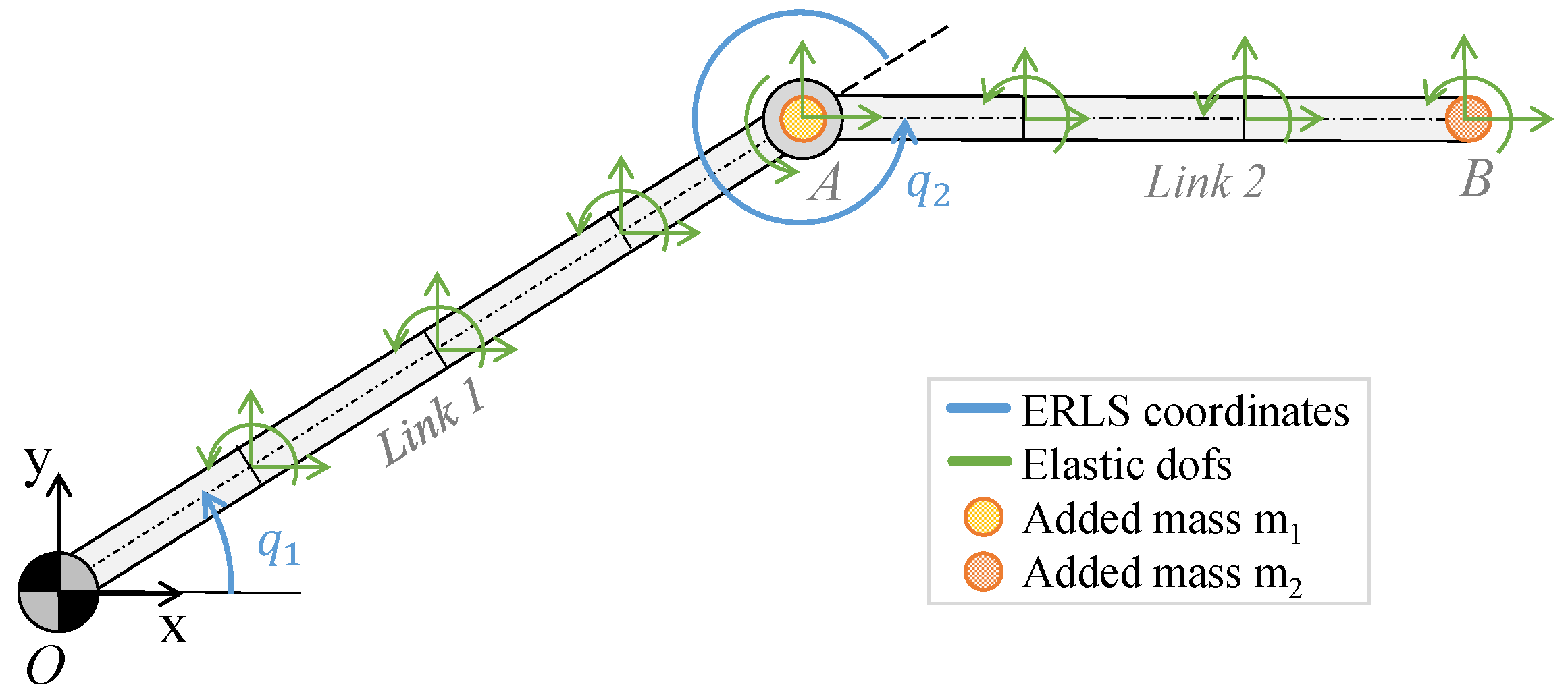
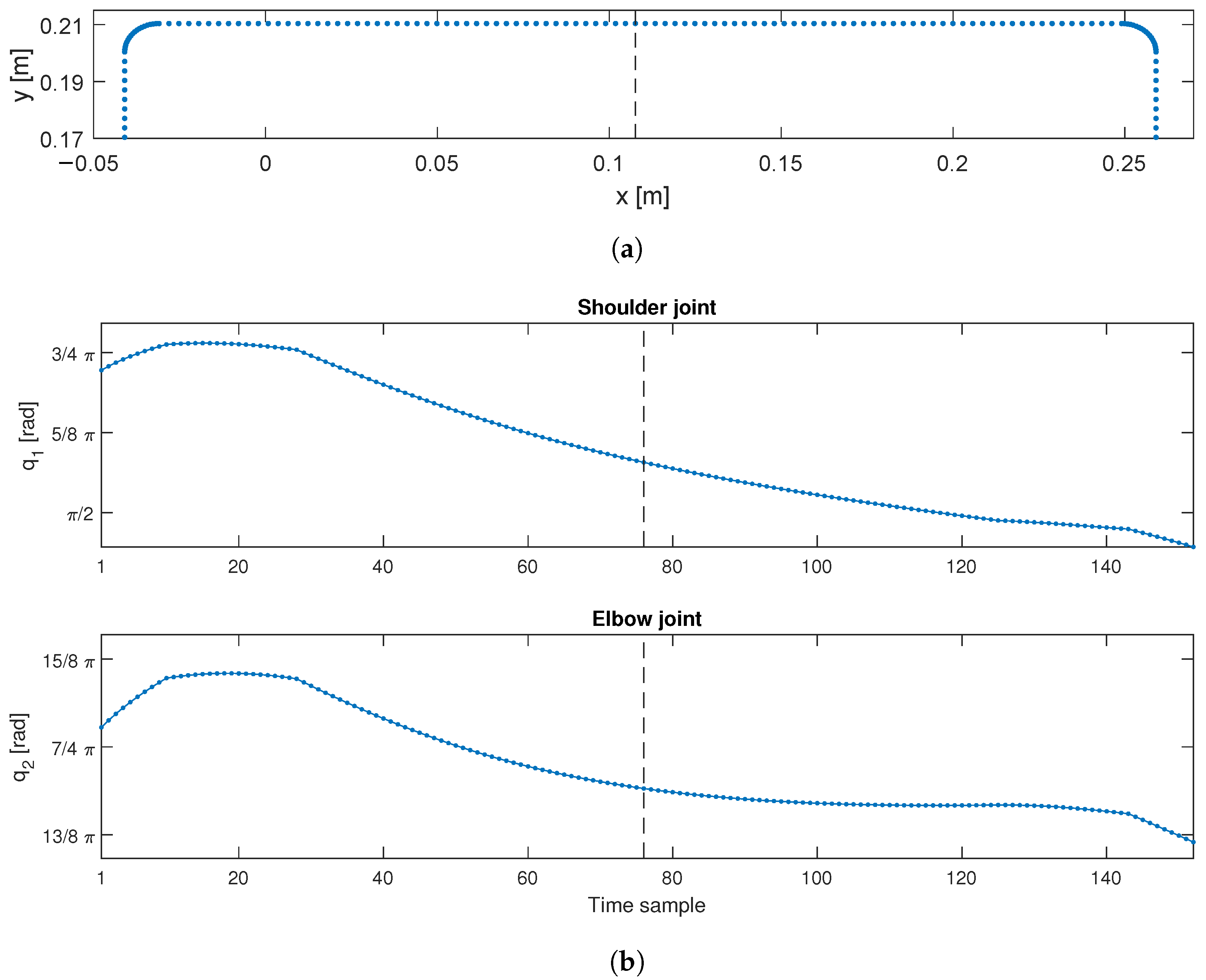
3.1. Description of a Benchmark Problem

The flexible-link multibody system considered for validation of the method is a planar two-link mechanism with two revolute joints, as shown in Figure 1. The geometric and physical properties of the system are listed in Table 1. Link 1 and link 2 are divided into four and three Euler–Bernoulli beam elements with circular and solid cross-sections, respectively. The resulting model has 23 degrees of freedom (dof), including the two rigid dofs of the ERLS, denoted by q 1 and q 2 , and 21 elastic dofs.
It is supposed that the end effector, denoted by symbol B in Figure 1, moves along the path shown in Figure 2a, which can be employed in a pick-and-place task. The trajectory is sampled at constant time intervals, where each dot in the figure represents a sample (152 samples in total). The inverse kinematics are solved, resulting in the joint-space trajectory shown in Figure 2b.
In this example, it is assumed that two point masses m 1 and m 2 can be placed on the elbow joint and end effector, respectively, if necessary to assign the desired eigenfrequency. Hence, y = m 1 m 2 T . The choice of the design variable y is arbitrary, as long as it is consistent with the ERLS model previously described, but it must be determined prior to optimization. In order to preserve the integrity of the FLMS, the design parameters are subjected to the following constraint set:
m 1 , m 2 : 0 m 1 0.250 kg , 0 m 2 0.250 kg .

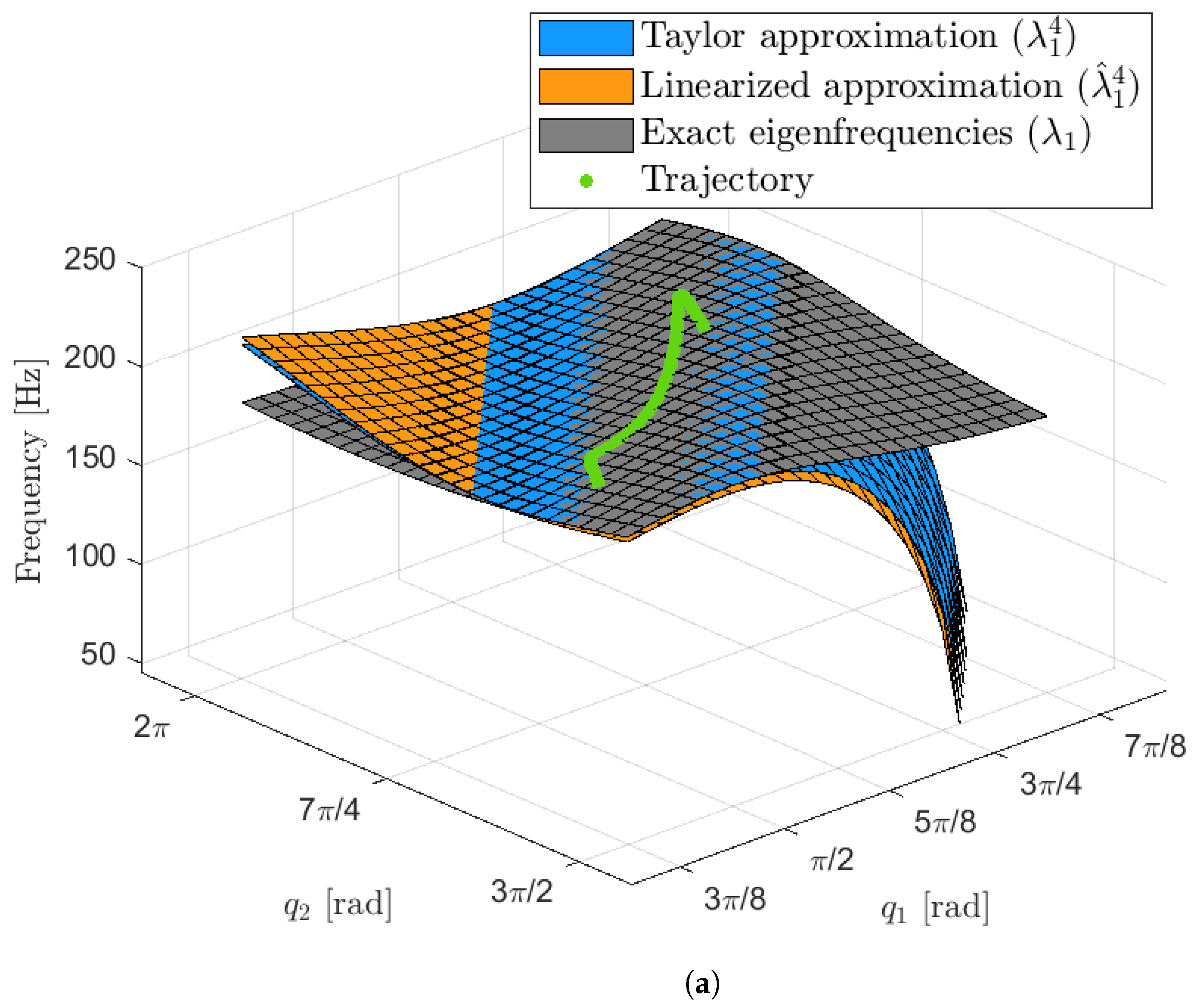
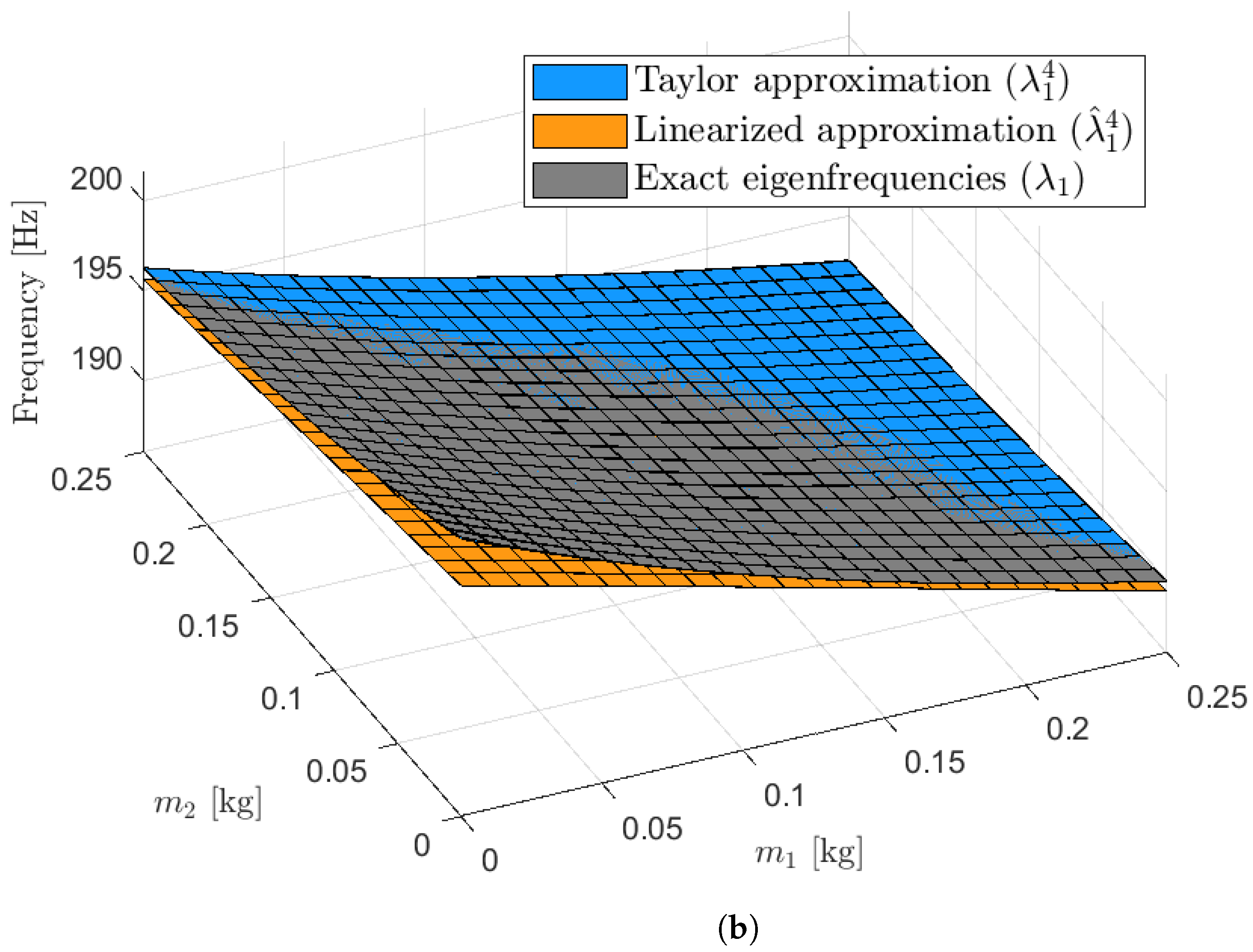
3.2. Parameter Study Results

Before attempting eigenfrequency assignment, the accuracy of the approximation of the eigenfrequencies provided by the Taylor expansion must be assessed. The expansion point q 0 , y 0 has been chosen as q 0 = 1.817 rad 5.312 rad T , which corresponds to the dashed lines, approximately in the middle of the trajectory in Figure 3, and y 0 = 0.125 kg 0.125 kg T , which is halfway between the upper and lower bounds of Equation (15).
The 4th order Taylor polynomial ( p = 4 ) of the lowest eigenfrequency ( i = 1 ), i.e., λ 1 4 q , y , and the partially linearized polynomial, i.e., λ ^ 1 4 q , y , are compared with the actual eigenfrequency of the multibody system. For clarity of representation, the approximations are compared in two ways. In Figure 3, variable q varies in the domain 3 π / 8 , 7 π / 8 × 3 π / 2 , 2 π , while y is fixed at the value 0 0 T (no point masses are added at the joints). If the comparison is restricted to the points of the trajectory, represented in the figure by the green line, the maximum relative error is 0.09 % for λ 1 4 and 1.64 % for λ ^ 1 4 .
In Figure, variable q is fixed at the value q 0 (same position as the expansion point), while y varies in the domain 0 , 0.250 × 0 , 0.250 . The maximum relative error of λ 1 4 is 0.05 % , while λ ^ 1 4 has a maximum relative error of 1.34 % in the considered domain. The assessment of the relative error demonstrates that the partially-linearized polynomial λ ^ 1 4 can approximate the considered eigenfrequency with sufficient accuracy. In fact, the presence of small model uncertainties affects, but does not compromise, the attainment of the desired eigenfrequencies.

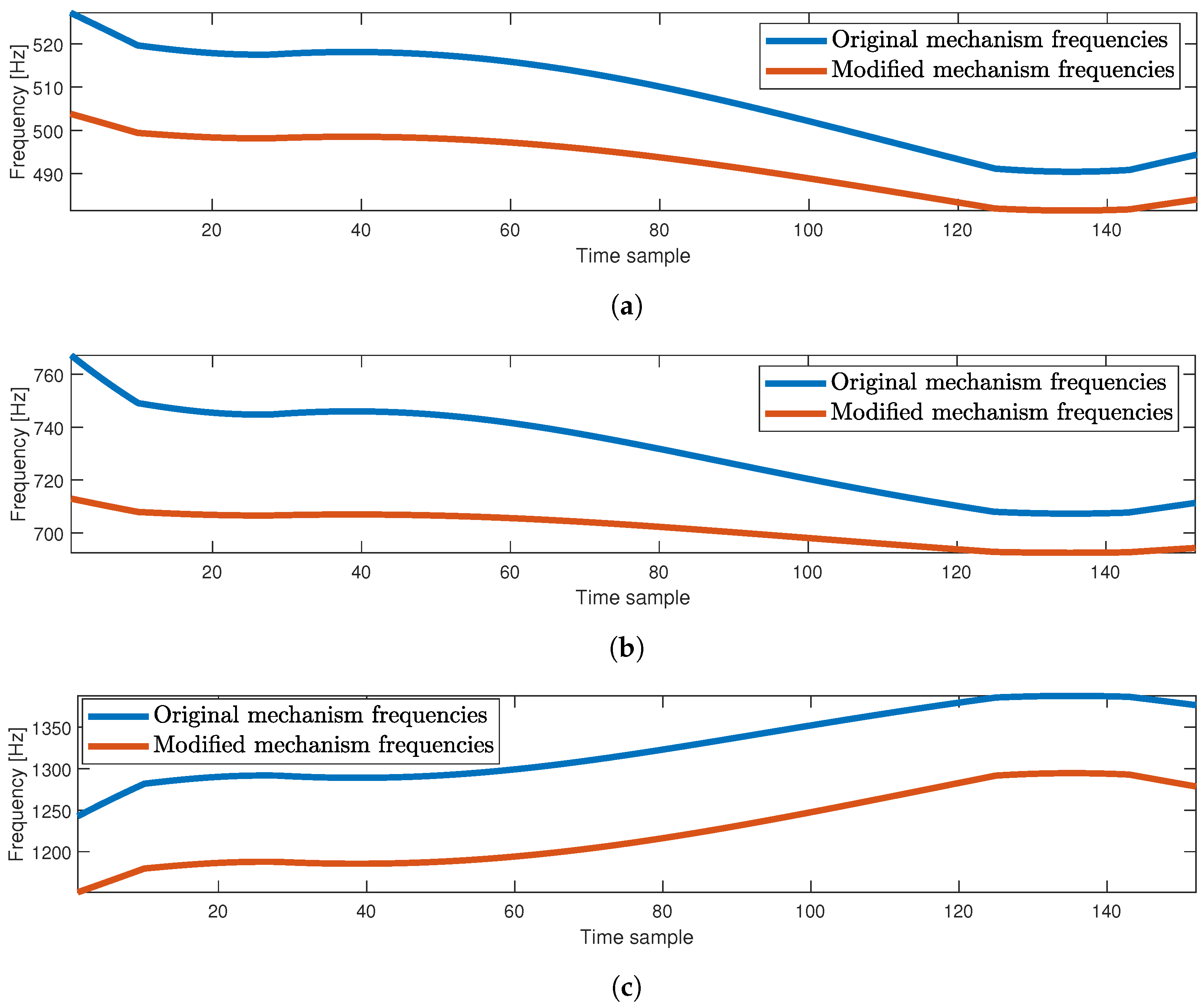
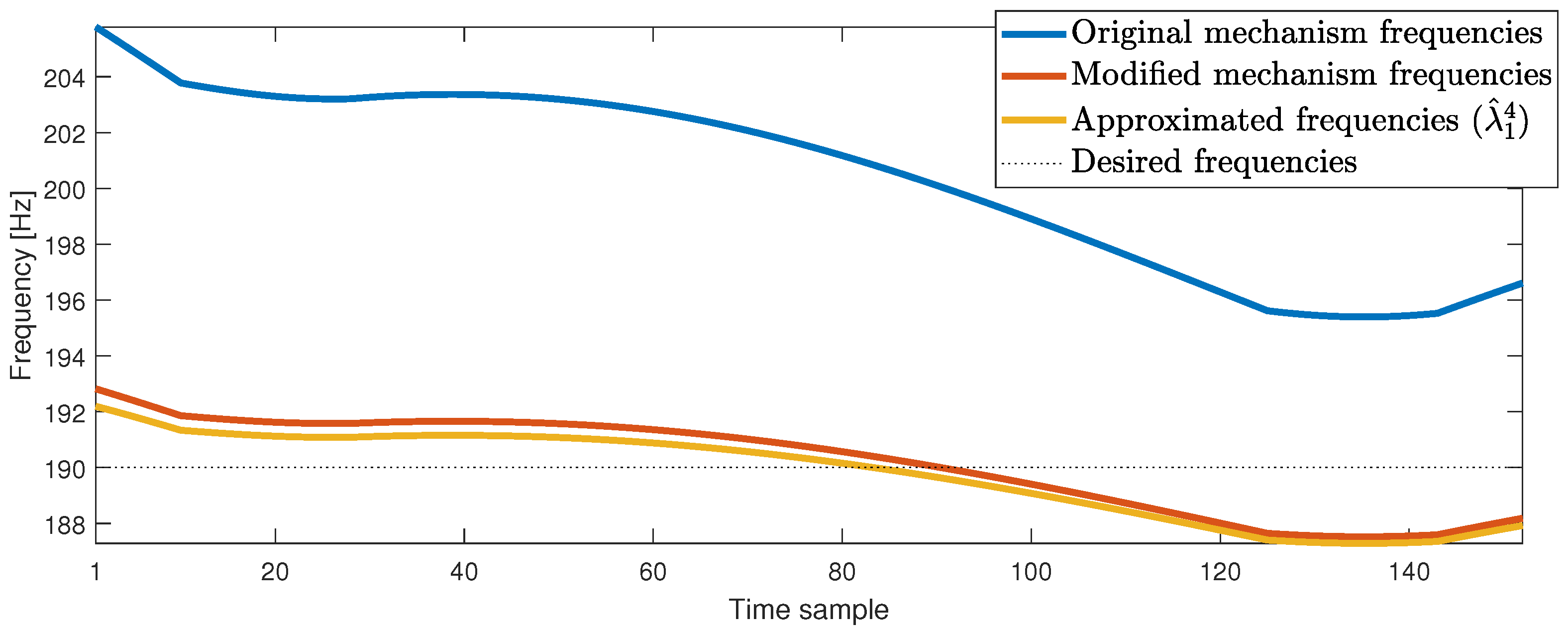
3.3. Optimum Design Results

The method is challenged with the following objective: modify the considered FLMS in such a way that the lowest eigenfrequency becomes λ 1 , d t 190 H z , t 0 , T . The integrals in (13) and (14) are computed numerically by using the trapezoidal rule on the same grid as for the discretization of the trajectory q t (in Section 3.1 and Figure 3). The constraint set Γ is chosen consistently with (15) as
Γ = δ m 1 , δ m 2 : 0.125 kg δ m 1 0.125 kg , 0.125 kg δ m 2 0.125 kg .
If δ y belongs to the set Γ , it is said to be feasible. The optimization problem (11) is solved using the quadprog function from MATLAB’s Optimization Toolbox. The interior-point-convex algorithm converges rapidly in 6 iterations with optimality tolerance set to 10 8 . The optimal value is obtained as δ y = 0.1004 0.1250 T , which translates to m 1 = 0.2254 kg and m 2 = 0 .
The eigenfrequencies are compared in Figure 4. The eigenfrequencies of the modified FLMS are closer to the desired frequency λ 1 , d than the ones of the original system. In fact, the maximum relative error for the original mechanism is 8.31 % , which is reduced to 1.48 % in the modified system. Such a result demonstrates that eigenfrequencies can be effectively assigned by means of the proposed method.
It must be noted that the modification of the system also affects the eigenfrequencies higher than the first. The change in such frequencies can be assessed from Figure 5, in which the frequency of the second, third and fourth mode are shown.

4. Conclusions

In this work, a method is proposed for designing flexible-link multibody systems to feature a desired eigenfrequency. The method exploits the ERLS formulation of dynamic equations, which is parametric in the mechanism configuration q . therefore, it is possible to calculate the derivatives of the system matrices M and K analytically. Hence, the Taylor polynomial of the eigenfrequency and eigenvector are computed by means of an iterative process. The obtained approximation of the eigenfrequency is linearized with respect to the design variables in order to recast the eigenfrequency assignment problem as a quadratic optimization program, which is tractable from the numerical point of view.
The application to a two-dof serial manipulator with flexible links, supposed to perform a pick-and-place motion, proves that it is possible to shift the lowest eigenfrequency closer to a target value. This numerical validation shows the numerical reliability and fast convergence of the method, making the proposed approach appealing for eigenfrequency assignment of large-scale FLMS. Such systems will be addressed in future work, as well as the validity of the partial linearization with respect to large displacements of multibody systems and large changes in the design variables.

Author Contributions

Conceptualization, R.B., I.P. and E.W.; methodology, R.B., I.P. and E.W.; software, R.B. and I.P.; supervision, E.W., I.P. and R.V.; validation, R.B.; writing—original draft, R.B., I.P. and E.W.; writing—review and editing, R.B., I.P., E.W. and R.V. All authors have read and agreed to the published version of the manuscript.

Funding

The research leading to these results can be framed within the COVI project (TN200Y) Free University of Bozen-Bolzano.

Institutional Review Board Statement

Not applicable.

Informed Consent Statement

Not applicable.

Data Availability Statement

The data presented in this study are available on request from the corresponding author.

Conflicts of Interest

The authors declare no conflict of interest.

References

  1. Braun, S.; Ram, Y. Modal modification of vibrating systems: Some problems and their solutions. Mech. Syst. Signal Process. 2001, 15, 101–119. [Google Scholar] [CrossRef]
  2. Liangsheng, W. Direct Method of Inverse Eigenvalue Problems for Structure Redesign. J. Mech. Des. Trans. ASME 2003, 125, 845–847. [Google Scholar] [CrossRef]
  3. Gladwell, G.M.L. Inverse Problems in Vibration. Appl. Mech. Rev. 1986, 39, 1013–1018. [Google Scholar] [CrossRef]
  4. Mottershead, J.; Ram, Y. Inverse eigenvalue problems in vibration absorption: Passive modification and active control. Mech. Syst. Signal Process. 2006, 20, 5–44. [Google Scholar] [CrossRef]
  5. Belotti, R.; Caracciolo, R.; Palomba, I.; Richiedei, D.; Trevisani, A. An Updating Method for Finite Element Models of Flexible-Link Mechanisms Based on an Equivalent Rigid-Link System. Shock Vib. 2018, 2018, 1797506. [Google Scholar] [CrossRef]
  6. Richiedei, D.; Tamellin, I.; Trevisani, A. Simultaneous assignment of resonances and antiresonances in vibrating systems through inverse dynamic structural modification. J. Sound Vib. 2020, 485, 115552. [Google Scholar] [CrossRef]
  7. Richiedei, D.; Tamellin, I.; Trevisani, A. A homotopy transformation method for interval-based model updating of uncertain vibrating systems. Mech. Mach. Theory 2021, 160. [Google Scholar] [CrossRef]
  8. Palomba, I.; Vidoni, R. Flexible-link multibody system eigenvalue analysis parameterized with respect to rigid-body motion. Appl. Sci. 2019, 9, 5156. [Google Scholar] [CrossRef] [Green Version]
  9. Turcic, D.A.; Midha, A. Generalized Equations of Motion for the Dynamic Analysis of Elastic Mechanism Systems. J. Dyn. Syst. Meas. Control 1984, 106, 243–248. [Google Scholar] [CrossRef]
  10. Vidoni, R.; Gallina, P.; Boscariol, P.; Gasparetto, A.; Giovagnoni, M. Modeling the vibration of spatial flexible mechanisms through an equivalent rigid-link system/component mode synthesis approach. JVC/J. Vib. Control. 2017, 23, 1890–1907. [Google Scholar] [CrossRef]
  11. Myers, R.; Montgomery, D. Response Surface Methodology: Process and Product Optimization Using Designed Experiments, 2nd ed.; Wiley: Hoboken, NJ, USA, 2002. [Google Scholar] [CrossRef]
  12. Krige, D.G. A statistical Approach to Some Mine Valuations and Allied Problems at the Witwatersrand. Master’s Thesis, University of Witwatersrand, Johannesburg, South Africa, 1951. [Google Scholar]
  13. Forrester, A.I.; Keane, A.J. Recent advances in surrogate-based optimization. Prog. Aerosp. Sci. 2009, 45, 50–79. [Google Scholar] [CrossRef]
  14. Huang, Z.; Wang, C. Optimal design of aeroengine turbine disc based on Kriging surrogate models. Comput. Struct. 2011, 89, 27–37. [Google Scholar] [CrossRef]
  15. Xu, Q.; Wehrle, E.; Baier, H. Adaptive surrogate-based design optimization with expected improvement used as infill criterion. Optimization 2012, 61, 661–684. [Google Scholar] [CrossRef]
  16. Boursier Niutta, C.; Wehrle, E.J.; Duddeck, F.; Belingardi, G. Surrogate modeling in design optimization of structures with discontinuous responses: A new approach for ill-posed problems in crashworthiness design. Struct. Multidiscip. Optim. 2018, 57, 1857–1869. [Google Scholar] [CrossRef]
  17. Duddeck, F.; Wehrle, E.J. Recent advances on surrogate modeling for robustness assessment of structures with respect to crashworthiness requirements. In Proceedings of the 10th European LS-DYNA Conference, Wrzburg, Germany, 15–17 June 2015. [Google Scholar]
  18. Shabana, A.; Zaher, M.; Recuero, A.; Rathod, C. Study of nonlinear system stability using eigenvalue analysis: Gyroscopic motion. J. Sound Vib. 2011, 330, 6006–6022. [Google Scholar] [CrossRef]
  19. Wittmuess, P.; Henke, B.; Tarin, C.; Sawodny, O. Parametric modal analysis of mechanical systems with an application to a ball screw model. In Proceedings of the 2015 IEEE Conference on Control Applications (CCA), Sydney, Australia, 21–23 September 2015; pp. 441–446. [Google Scholar]
  20. Palomba, I.; Vidoni, R.; Wehrle, E. Application of a parametric modal analysis approach to flexible-multibody systems. Mech. Mach. Sci. 2019, 66, 386–394. [Google Scholar] [CrossRef]
  21. Palomba, I.; Wehrle, E.; Vidoni, R.; Gasparetto, A. Parametric eigenvalue analysis for flexible multibody systems. Mech. Mach. Sci. 2019, 73, 4117–4126. [Google Scholar] [CrossRef]
  22. Floudas, C.A.; Visweswaran, V. Quadratic Optimization. In Handbook of Global Optimization; Springer: Boston, MA, USA, 1995; pp. 217–269. [Google Scholar] [CrossRef]
Figure 1. Finite element model of the flexible-link manipulator.
Applsci 11 11558 g001
Figure 2. Trajectory of the flexible linkage: (a) end-effector trajectory in the work space; (b) joint space trajectory.
Applsci 11 11558 g002
Figure 3. Comparison of approximated and exact eigenfrequency versus (a) generalized coordinates q and (b) design variables y .
Applsci 11 11558 g003aApplsci 11 11558 g003b
Figure 4. Comparison of original and optimal design.
Applsci 11 11558 g004
Figure 5. Comparison of the original and modified system eigenfrequencies in the (a) second mode; (b) third mode; (c) fourth mode.
Applsci 11 11558 g005
Table 1. System parameters of the two-link mechanism.
ParameterValue
Link 1 length 0.6 m
Link 2 length 0.45 m
Linear mass density1.9 kg/m
Young’s modulus 69 · 10 9 P a
Bending moment of inertia 3.97 · 10 4 m 4
Publisher’s Note: MDPI stays neutral with regard to jurisdictional claims in published maps and institutional affiliations.

