High-Resolution LiDAR Digital Elevation Model Referenced Landslide Slide Observation with Differential Interferometric Radar, GNSS, and Underground Measurements

Featured Application

Verification of DInSAR analysis results, Ascending or Descending solution for better aspect, GNSS verification method, underground to ground surface measurement, and landslide mapping based on deformation map.

Abstract

The area of Taiwan is 70% hillsides. In addition, the topography fluctuates wildly, and it is active in earthquakes and young orogenic movements. Landslides are a widespread disaster in Taiwan. However, landslides are not a disaster until someone enters the mountain area for development. Therefore, landslide displacement monitoring is the primary task of this study. Potential landslide areas with mostly slate geological conditions were selected as candidate sites in this study. The slate bedding in this area is approximately 30 to 75 degrees toward the southeast, which means that creep may occur due to gravity deformation caused by high-angle rock formation strikes. In addition, because the research site is located in a densely vegetated area, the data noise is very high, and it is not easy to obtain good results. This study chose ESA Sentinel-1 data for analysis and 1-m LiDAR DEM as reference elevation. The 1-m LiDAR DEM with high accuracy can help to detect more complex deformation from DInSAR. The Sentinel-1 series of satellites have a regular revisit period. In addition, the farm areas of roads, bridges, and buildings in the study area provided enough reflections to produce good coherence. Sentinel-1 images from March 2017 to June 2021 were analyzed, obtaining slope deformation and converting it to the vertical direction. Deformation derived from SAR is compared with other measurements, including GNSS and underground slope inclinometer. The SBAS solution process provides more DInSAR pairs to overcome the problem of tremendous noise and has increased accuracy. Moreover, the SBAS method’s parameter modification derives more candidate points in the vegetated area. The vertical deformation comparison between the GNSS installation location and the ascending SBAS solution’s vertical deformation is consistent. Moreover, the reliable facing of the slope toward the SAR satellite is discussed. Due to the limitations of the GNSS stations, this study proposes a method to convert the observed deformation from the slope inclinometer and convert it to vertical deformation. The displacement of the slope indicator is originally a horizontal displacement. It is assumed that it is fixed at the farthest underground, and the bottom-to-top movement is integrated with depth. The results show that the proposed equation to convert horizontal to vertical displacement fits well in this condition. The activity of landslides within the LiDAR digital elevation model identified as scars is also mapped.

1. Introduction

Taiwan is located at the boundary of two plates, where frequent earthquakes occur. The collision of plates also results in orogeny, increasing the height of mountains. Due to the island being surrounded by different seawater temperatures, the extreme weather changes very fast and induces numerous typhoons and rainfall. For example, in 2009, the highest accumulated rainfall in one typhoon event was 3000 mm. The amount was about three fourths of the average annual rainfall. These massive rainfall events are why such a small island covers many potential sliding slopes. Landslide hazard mitigation is an essential issue in Taiwan. Central Geological Survey started to map the large-scale landslide (deep-seated landslide) scars from LiDAR DEM in the past ten years after typhoon Morakot in 2009. The mapped landslide scars can be downloaded from the open data of the government (Available online: https://data.gov.tw/en (accessed on 1 June 2021)). The existing scars imply what year those landslide events occurred but cannot indicate current conditions. The prominent scars weere downloaded and mapped in detail by this study are as shown in Figure 1. The deep-seated scar was mapped by the criteria that the area should be larger than 10 ha. Thus, detailed investigation and mapping are done by this research. There are several minor scars and cracks found during field investigation and LiDAR DEM mapping. The geological formation of the study area is slate, which varies with different sandstone content. The formation of slate is facing southeast ranging from 20 to 70 degrees, which may induce slow sliding due to gravity. The deformation speed of these scars is the first key issue to installing the monitoring system or engineering treatment.

Generally, PSInSAR was a method to derive large area deformation such as ground subsidence or fault deformation [1,2,3,4,5,6,7,8,9,10,11,12,13,14] performed landslide velocity detection with PSInSAR and SBAS and concluded that PS can have more solved points than SBAS. However, Rao etal. [15] did not provide accuracy verification with these methods. Oliveira et al. [16] used TerraSAR-X SAR to detect landslide activity with PSInSAR and showed that it is possible to map active landslides. Ciampalini et al. [17] combined PSInSAR with the steepest slope velocity and its variance to refine the landslide susceptibility map. Hastaoglu et al. [18] used ENVISAT and GNSS data to verify PSInSAR accuracy. Ciampalini et al. [19] adopted sensors on buildings and PSInSAR for building deformation and risk classification. The resolution of reference DEM is also an important issue when doing PSInSAR. Ciampalini et al. [20] used 1 m airborne LiDAR and 20 m DEM to compare the results of PSInSAR and showed that higher resolution DEM is more suitable for the derivation of ground movement. Mateos et al. [21] combined UAV and PSInSAR for higher resolution DEM for coastal displacement detection. The displacement detected in Mateos et al. [21] is about 1.92 m in 8 years. The interferometric staking is also called A-DInSAR in recent years, including PSInSAR, SBAS, and so on [22,23]. In addition to the two methods mentioned above, another TCP-InSAR can perform continuous DInSAR analysis. TCP-InSAR uses a temporary coherence point selection technique and can estimate long-term surface deformation without performing a phase reduction procedure [24]. In addition, Ferretti1 et al. [25] also improved the PS-InSAR with poor results in mountainous areas or non-artificial structures by using a new algorithm to get better quality candidate points. This algorithm is called SqueeSAR. Peduto et al. [26] and used inclinometer measurements for landslide kinematic modeling. The method projected the velocity to the steepest slope direction and compared Envisat and Cosmos Skymed with PSISAR.

We tried to initiate this study with SBAS. The comparison of different measurements was carried out after the movement of the ground surface was confirmed. The deformation value and velocity prove the activeness and can provide information about the landslide mechanism. However, DInSAR should pay attention to the correctness of the large-area analysis of landslide displacement. Given this, converting the relative satellite deformation (LOS) to the vertical direction is the only feasible verification method. To extract the different displacement paths from time-series data, Pawluszek et al. [27] used the equation provided by Hanseen [28] to calculate displacements in three directions. The Hanseen [28] algorithm is based on the geometry of the transmission and the reflection direction of the SAR signal. The method used in this research is based on the exact procedure but using the commercial software SARScape.

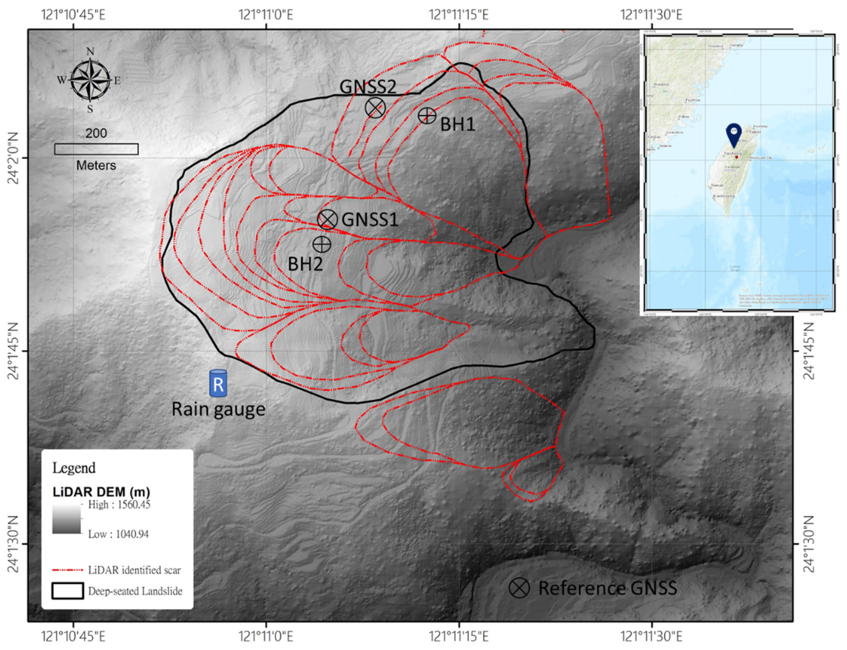
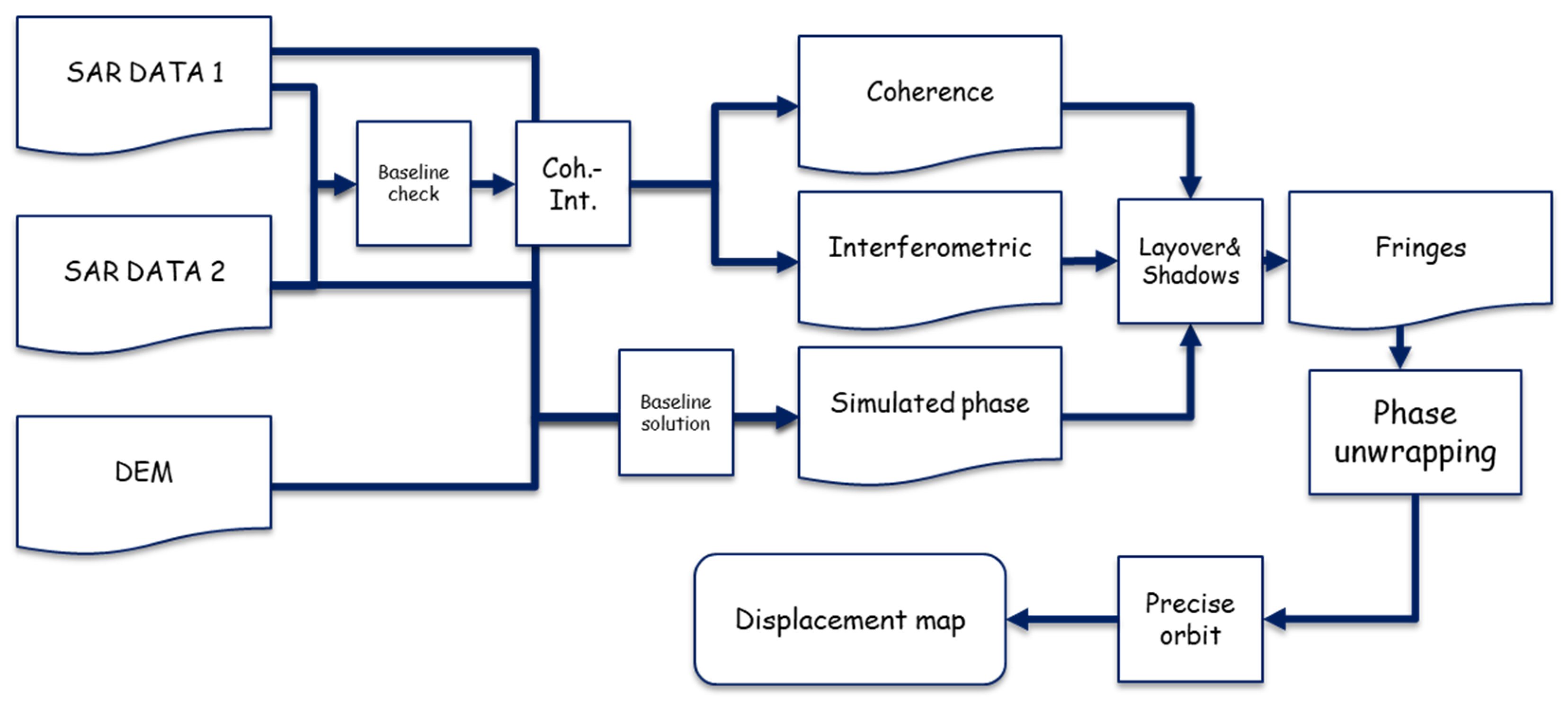
2. Materials and Methods

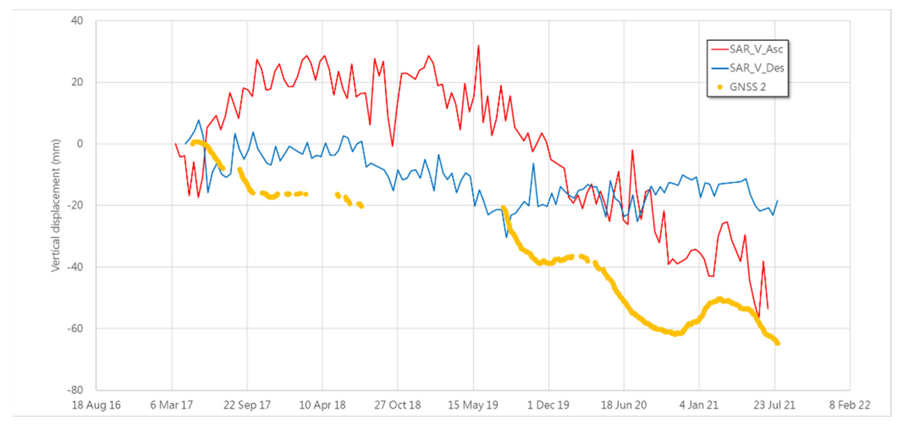
Vertical Deformation from DInSAR

The ground deformation can be obtained from the phase difference temporal SAR pairs. The basic concept is sending radar waves to the same position at different times and baselines. The phase differences of the two signals can be calculated with a reference digital elevation model. The control factors are accurate baseline and reflection on the ground surface. Moreover, precise orbit and reference DEM are also critical to finding actual deformation. DEM with 1 m resolution LiDAR DEM after the year 2009 is used as a reference in this study. The accuracy of ground deformation can be to less than a centimeter with the excellent quality of data, coherence, and amplitude. The phase difference of the interferogram cab is obtained by Equation (1). The actual ground deformation can be derived after removing known effects such as topography, geometry, and atmosphere. The atmosphere effect was eliminated by temporal scene filters without using any data from the meteorological station. Therefore, the interferometry can be calculated with a known baseline and reference height. The 1 m resolution LiDAR dem is adopted as reference height in this study.

$$\begin{gathered} {\varphi }_{Int}=4\pi \frac{R_1-R_2}{\lambda }={\varphi }_{Topography}+{\varphi }_{Movement}+{\varphi }_{Atmosphere} \\ =\frac{4{\pi \mathrm{B}}_{\mathrm{n}}}{\lambda R\sin \mathsf{\theta }}\mathrm{h}+\frac{4\pi }{\lambda }{\Delta R}_{Movement}+{\varphi }_{Atmosphere} \\ =\frac{4{\pi \mathrm{B}}_{\mathrm{n}}}{\lambda R\sin \mathsf{\theta }}\mathrm{h}+\frac{4\pi }{\lambda }{\Delta \mathrm{R}}_{Movement}+{\varphi }_{Noise} \end{gathered}$$

(1)

in which R: distances between satellites and observation location; B: baseline; h: reference elevation; λ: wavelength of the radar; θ: looking angle to the observation location.

DInSAR, PS InSAR, and SBAS InSAR were developed very fast in recent years. These technologies are becoming more efficient for large-scale landslide monitoring. Various methodologies have been proposed for faster processing and better results [29,30,31,32,33,34,35,36,37,38].

The reflection signal is feeble when a smaller wavelength sends it to the ground surface. This study uses single polarization (HH) for the same purpose a stronger reflection signal after testing in this area. The Sentinel-1 data was used for this research. The process to obtain DInSAR vertical displacement is shown in Figure 2 using only two temporal pairs and 1 m resolution LiDAR DEM to generate a simulated phase. The SAR processing software in this research is based on SARScape/ENVI. First, use the SAR images and DEM to produce coherence, interferometry, and simulated phase. After that, it eliminates layover and shadows from interferometry. However, the interferometry ranges from π to −π and the actual deformed phase is more than that. Thus, phase unwrapping is necessary for absolute phase differences. The final step is using GCP and precise orbit to convert the deformed phase to displacement.

The DInSAR method is suitable to observe landslide scars at two scenes with a short baseline and short period. However, the coherence, amplitude, and fringes derived from two images are hard to continuously monitor for displacement. Thus, interferometric stacking is introduced for the study area. PSInSAR and SBAS are adopted in this area, but the PSInSAR result has much fewer candidate points. The number of candidate points extracted from PSInSAR is only 1/10 of SBAS. Thus, only SBAS is shown in this study.

SBAS searches candidates with a similar radar signal amplitude by observing years and tracking their location in each scene. The atmosphere effect in this analysis is merely using temporal days and filters to eliminate. This study uses the European Space Agency (ESA) Sentinel-1 images due to its regular and 12 days return period. The temporal and space baseline is as shown in Figure 3. The temporal baseline is set to 60 days, and the space baseline is set to 150 m in this study. The images of ascending and descending used in this study are 126 and 121 images, respectively.

The RMS vertical displacement error directly from SARScape shows 8.6 mm with 95% confidence in ascending track and 9.8 mm with 95% confidence in descending track. The azimuth angle of the incident angle of the ascending orbit is 80.1 degrees, and the inclination angle is 39.1 degrees. The azimuth angle of the incident angle of the descending orbit is 281.5 degrees, and the inclination angle is 36.9 degrees. The aspect of the study area is mainly in the east direction. The aspect (azimuth) and slope (steepness) affect candidate point numbers and their accuracy. There are more candidate points derived from ascending track images, as shown in Figure 4. This is because the slope of the study area is facing the ascending SAR satellite signal. Also, some parameters of SARScape are optimized for the study area to produce the most candidate points. However, the next step is to verify the accuracy of each of the track results in this study area.

3. Results

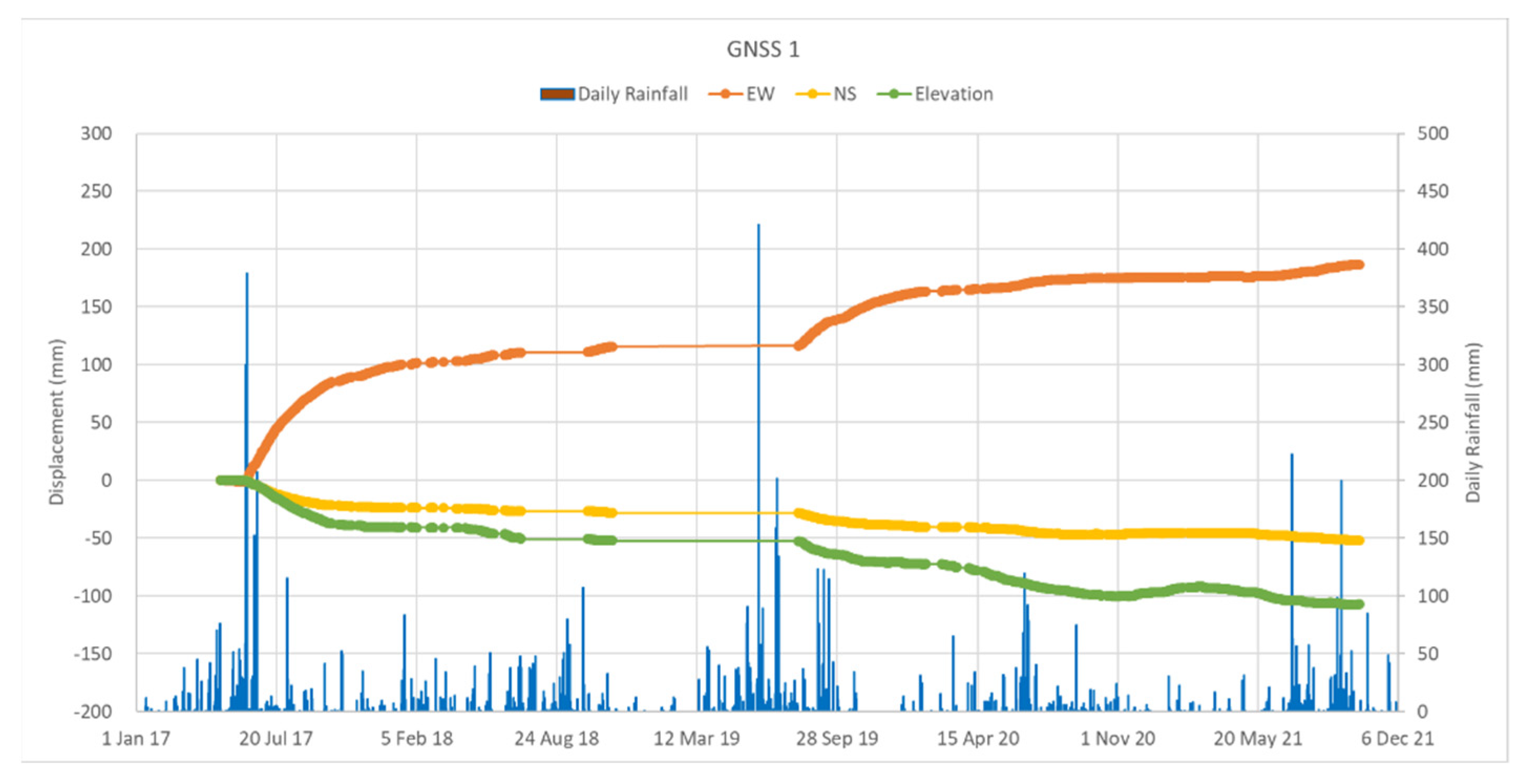
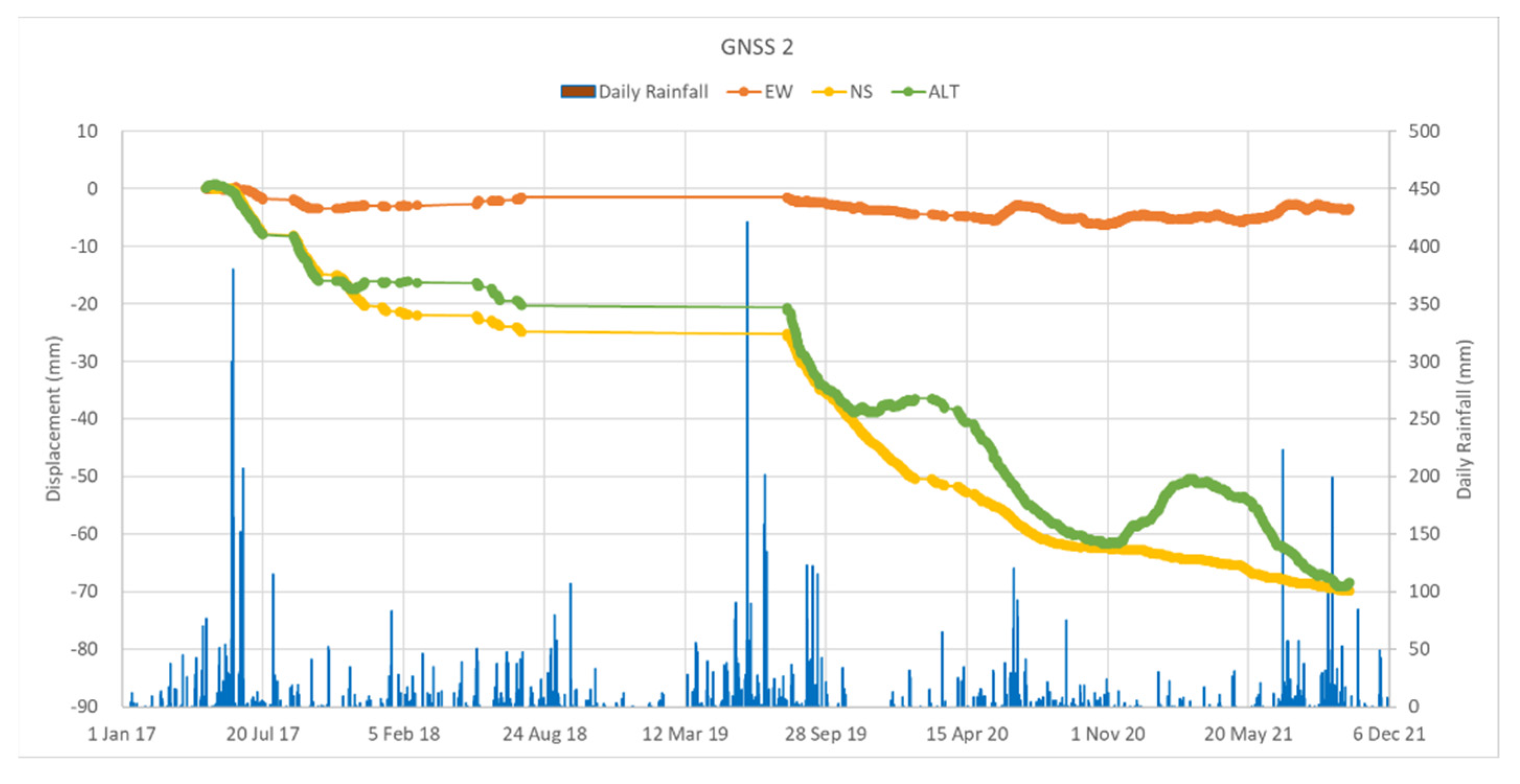
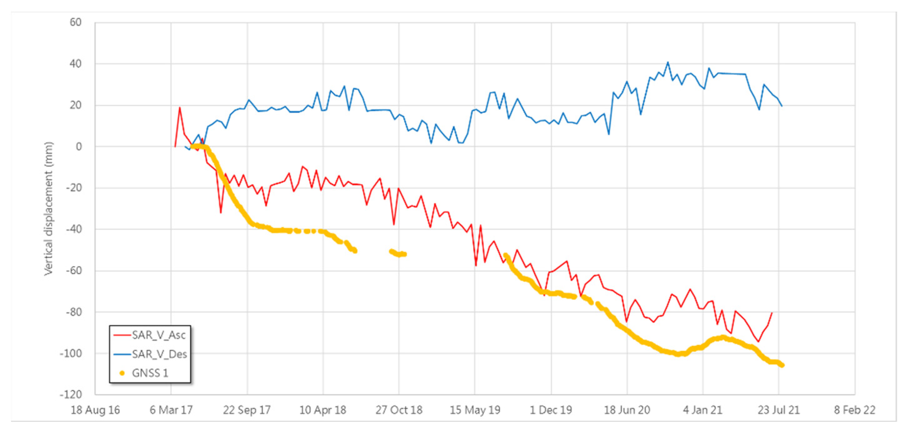
3.1. GNSS Measurement

Two dual-frequency GNSS stations were installed for analysis to verify the accuracy of the SBAS analysis results, as shown in Figure 1 from April 2017. A reference GNSS station located at a stable place 1.1 km away from this point is adopted for a node to node displacement calculation. Assuming the reference GNSS station is stable without displacement. The selection of GNSS station sites was based on preliminarily DInSAR analysis. The differential GNSS calculation is based on open source code RTKLIB. The road could be blocked due to heavy rainfall. Thus, the recorded data was sent through the internet to the lab and calculated on another server every hour. The return period of Sentinel-1 data is 12 days. The hourly solution is too much for DInSAR verification. Thus, a 24 h solution is adopted as well.

As shown in Figure 5 and Figure 6, there are two significant events from April 2017 to June 2021. The first event hit this area in June 2017, just two months after the GNSS stations were installed. The rainfalls hit in June 2017. The first event (1st June to 4th June) has 902.5 mm rainfall and 640 mm rainfall after several days (11th June to 18th June). This event induced about 120 mm in the east direction, 38 mm in the south direction, and 78 mm in the vertical direction at GNSS1. There is another significant rainfall event in 2019. The hourly rainfall reached a peak of 52 mm, but accumulated rainfall was less than the event in 2017. However, displacements were measured in this event. The south direction displacement at GNSS2 is more than east since its slope direction is heading south. The horizontal displacement at GNSS2 is almost the same as vertical displacement. But the horizontal displacement at GNSS1 is much more than vertical displacement. The displacement result means that the location of GNSS2 is at a single sliding surface and GNSS1 is at multiple sliding surfaces, which means there is a deeper sliding surface underneath. The field identification and numerical simulation are executed to verify this observation.

The vertical displacement is adopted for verification. Vertical displacements at GNSS1 and GNSS2 are extracted for SBAS SAR comparison, as shown in Figure 7 and Figure 8. GNSS1 vertical displacement is very consistent with ascending SBAS within centimeter accuracy. The descending SBAS is quite different from actual displacement behavior owing to topography. This result shows that the aspect of the mountain is controlling the selection of tracks to analyze landslide behavior. The GNSS2 is installed inside Lushan elementary school with a slope facing south. The comparison results show that the descending track is more consistent than the ascending track. However, the ascending track has more accurate displacement after four years of waiting. Thus, the following result discussion will focus on the ascending track in this study area. Moreover, it is interesting that both GNSS and SBAS measured uplift after the main events in 2017. The mechanism will be discussed in the next section.

The slope (steepness) and aspect (azimuth) of GNSS stations are shown in

Table 1. The slope (steepness) and aspect (azimuth) of GNSS stations and related DInSAR comparison errors.

	GNSS1 Location
	Slope (degree)	Aspect (degree)
	15.6	88.9
	Ascending orbit	Descending orbit
Error Mean (mm)	13.21	84.74
Error Standard Deviation (mm)	10.14	37.82
Correlation coefficient	0.95	−0.69
	GNSS2 Location
	Slope (degree)	Aspect (degree)
	19.8	169.8
	Ascending orbit	Descending orbit
Error Mean (mm)	24.43	25.76
Error Standard Deviation (mm)	15.17	17.52
Correlation coefficient	0.51	−0.20

. For the accuracy of DInSAR results, the GNSS measurements are adopted as an exact reference. Only the data on the same day of the DInSAR result and GNSS solution is used. As shown in Table 1 of GNSS1 data, the ascending orbit result shows a 13 mm error with a 10 mm standard deviation. Moreover, the correlation coefficient is 0.95, which means highly correlated. For the descending orbit at GNSS1, the error is 84 mm. The correlation coefficient is −0.69, which implies that descending data cannot be used in this location. For the site of GNSS2, the error and standard deviation of ascending data are more significant than GNSS1, but the correlation coefficient is only 0.51. The result shows that the DInSAR result is still applicable at this location with lower accuracy. The descending data also shows low accuracy and is not appropriate at this location. The correlation coefficient is the relation between the GNSS and DInSAR measurements. If the coefficient approaches one, this indicates that these two data are the same.

On the other hand, if the coefficient is less than zero, this means completely different results and even indicates minor mean errors. Thus, we can conclude that ascending SAR data is better than descending SAR data in this study area. The results show that ascending SAR data is suitable for the east aspect slope.

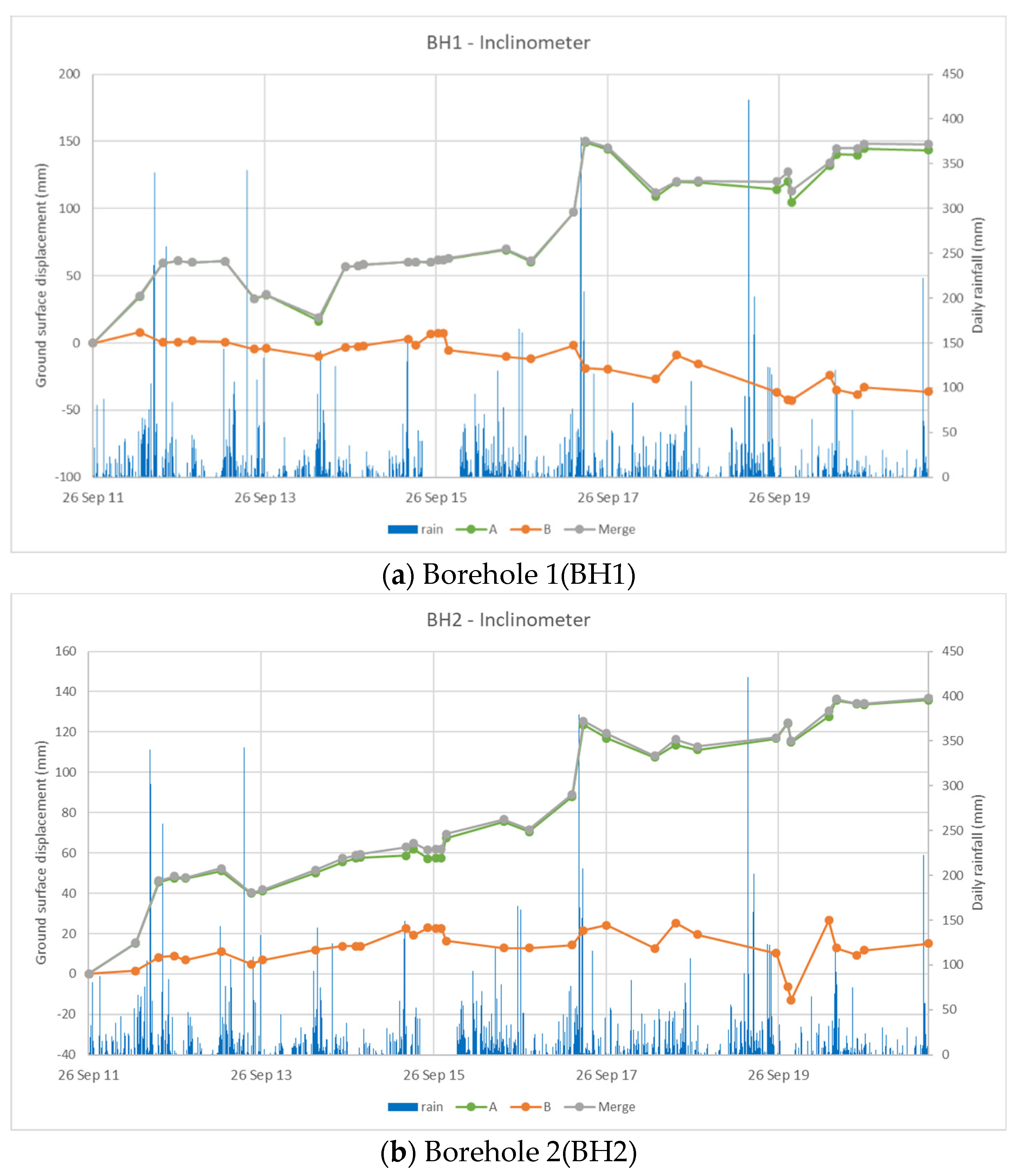
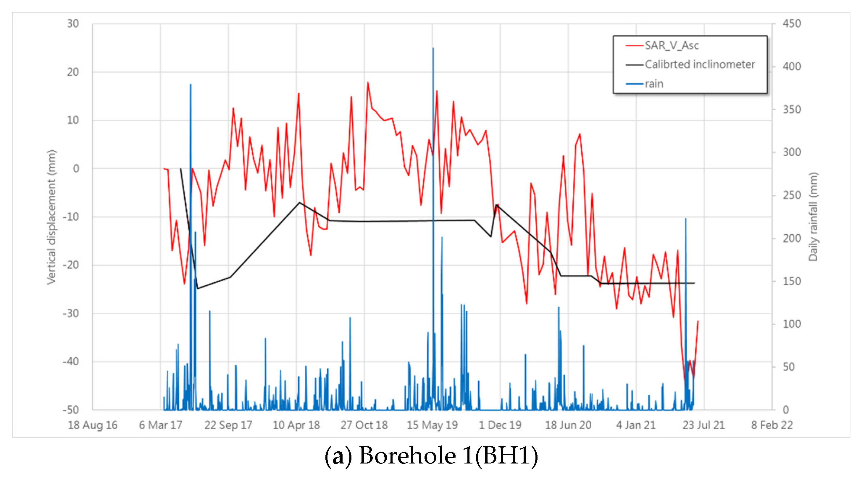
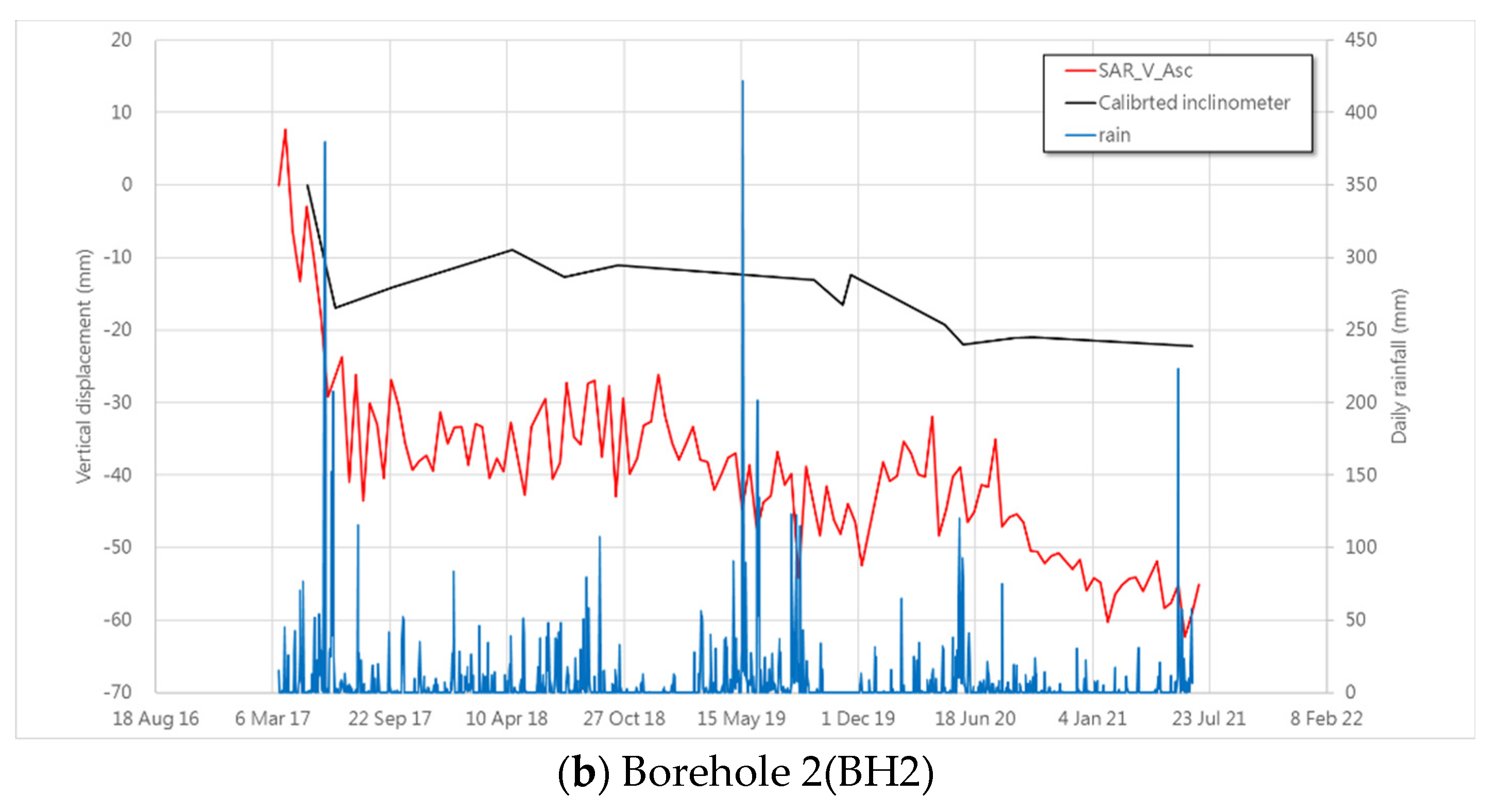
3.2. The Sliding Behavior Comparing with Slope Inclinometer

The study site was investigated for more than ten years. However, the continuous GNSS measurement was quite expensive before that. The borehole is the traditional method to understand underground geology and deformation measurement. Two boreholes, BH1 and BH2, are adopted in this study, as shown in Figure 1. The depths of BH1 and BH2 are 100 m and 80 m, respectively. The measurement of deformation is initiated from the far bottom of the hole. The algorithm assumes that the far bottom is not moving and measures the tilt angle in two perpendicular directions tilt angle. Then the horizontal displacement at each depth can be derived by tilt angle times depth. The horizontal displacement can be used as a reference compared with the SBAS method when the GNSS is limited. The horizontal ground surface displacements are plotted in Figure 9 with daily rainfall. There are two horizontal directions measured, which are A direction and B direction. The two directions are perpendicular to each other. The direction of horizontal displacement is hard to identify because the underground pipe could be twisted. Thus, we merge two directions into one displacement. The results show that A direction is a controlled direction in this case. The slope inclinometer was initiated to measure from 2011. There were two significant events in 2012 and 2017, respectively. The two events were caused by heavy rainfall of more than 1000 mm. Because SBAS can only detect ground deformation, this study uses ground surface displacements with time as a reference.

A concept to convert horizontal displacement to vertical displacement is proposed in this research. The idea of this concept is shown in Figure 10. The slope indicator measures a horizontal displacement in referenece to the deep ground surface. With an average slope at the hole, the vertical displacement at the same point can be estimated based on Equation (2). The recommended distance (radius) to calculate slope degree is from the center of the hole to the radius larger than the depth of the inclinometer.

$$\tan \theta =\frac{V}{H}\to V=H\times \tan \theta$$

(2)

where, θ: average slope at slope indicator; H: ground surface displacement from slope indicator; V: estimated vertical displacement.

The converted vertical displacement is plotted in Figure 11. The vertical movement derived from ESA Sentinel-1 is also plotted in the same period to compare. The result shows that this method can be used for estimating the vertical displacement trends correctly at BH1. However, the displacement comparison at BH2 is only consistent with the deformation trend, not accurate. The method proposed is based on landslide monitoring, in which the observation point is moving down in general. The process should be carefully checked in case the observation point is moving up (uplift). This method allows comparing DInSAR and slope indicator data, especially traditional monitoring sites without GNSS or leveling data. There are two interesting observations when comparing these locations. The first one is that the deformation was reversed after the 2017 event. And the second one is that these locations are not affected by the 2019 event.

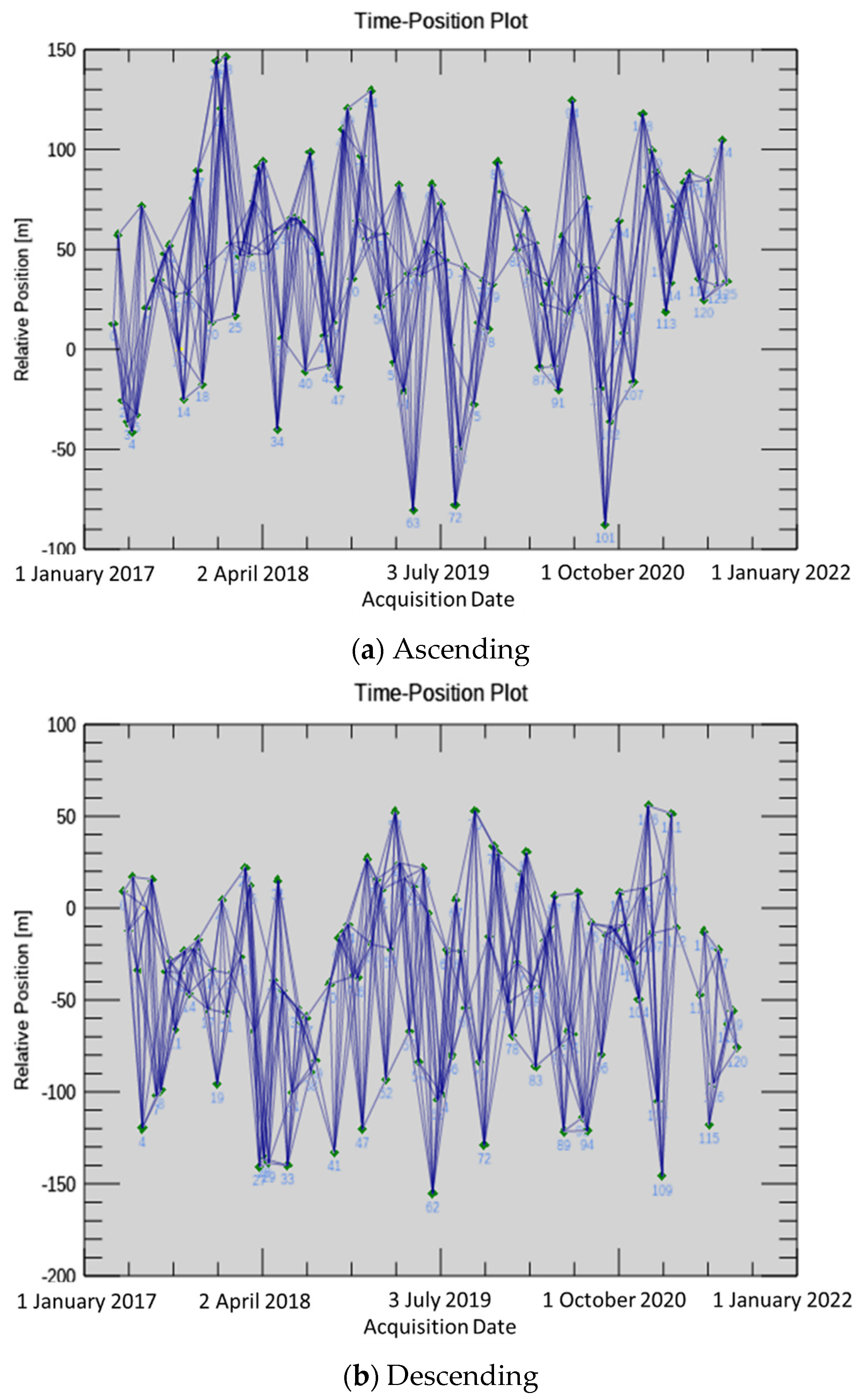
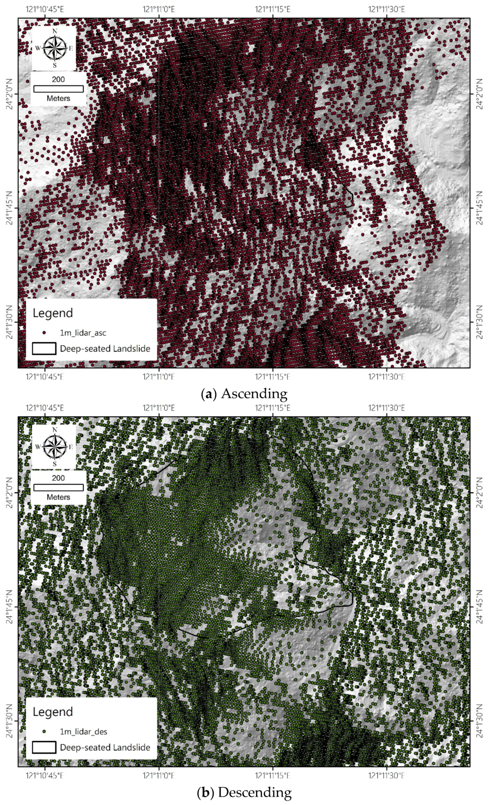
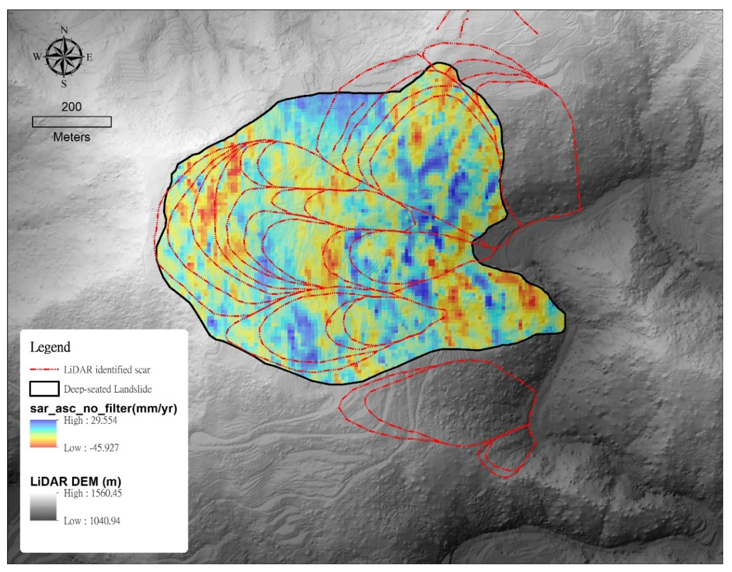
3.3. Potential Landslide Scar Mapping from SBAS Method

Since the accuracy of the SBAS method is verified in this area with GNSS and slope inclinometer, landslide mapping based on this method is possible in the study area. In order to set up a standard operating procedure to map the landslide area, the following steps are executed after several tests.

1.

Calculate vertical displacement from LOS displacement after SBAS analysis.

2.

Interpolate vertical displacement to raster format.

3.

Overlap raster vertical displacement with shaded hill derived from the digital elevation model.

4.

Compare displacement with LiDAR identified scars.

The potential landslide scars are mapped after the procedures, as shown in Figure 12. The landslide scars from LiDAR are also shown in the figure to compare the differences. The figure shows that most of the LiDAR base landslide area is moving, which means mapping landslides from LiDAR data is correct. However, the sliding displacement also means the priority to do further monitoring or engineering treatment. The SBAS method shows a possible procedure to select sites for hazard mitigation. The method based on this research mapped more potential landslides than LiDAR mapped landslides. These potential landslides are moving, but the sliding threshold is difficult to define due to continuous regular sliding. The primary observation from this LiDAR DEM-based SBAS deformation shows that most of the sinking displacement occurs at the mapped scar’s crown. Also, some uplift deformation can be observed at a lower elevation of the slope.

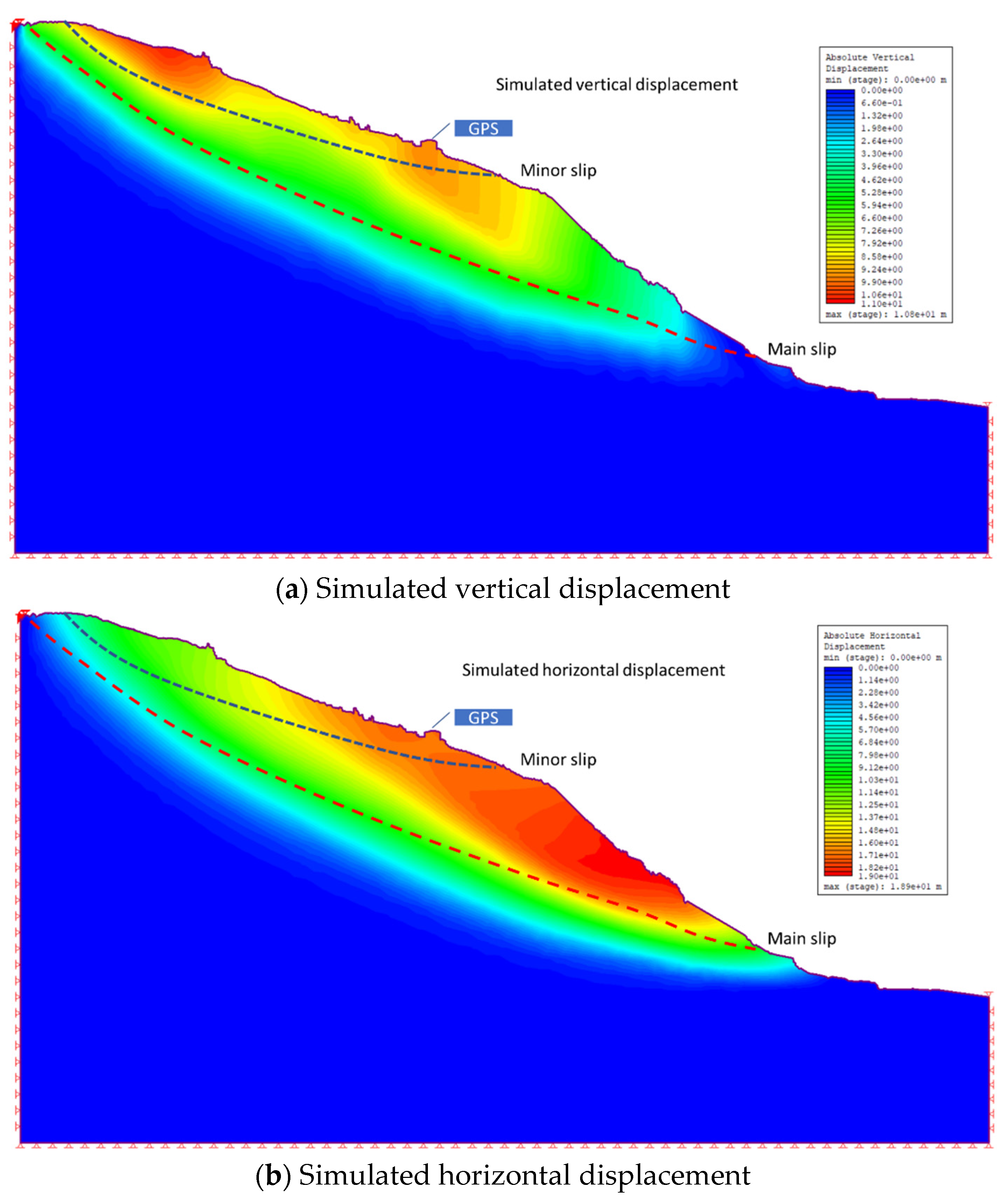
3.4. Numerical Simulation and Field Investigation of Uplift Condition

Vertical displacement in the previous figure (Figure 5) shows an uplift behavior after the severe rainfall event in 2017. The observation from GNSS1 indicates that the horizontal displacement is much larger than the vertical displacement. The minor effect detected means there are multiple sliding planes. Field investigation in this site is checked to find the sliding mechanism. Figure 13 shows the crack in the wall, where a GNSS was installed at the top of the roof. The displacement of the retaining wall to the bottom is larger than the top, illustrating a circular failure condition, which may have resulted in rotation with higher elevation at the sliding toe. In order to simulate this condition, a simple slope model was adopted for finite-element analysis RS2 from Rocscience is adopted for finite-element analysis. A profile from crest to toe was cut to simulate landslide displacement. The simulated result is as shown in Figure 14. The GNSS location is indicated in the plot. Simulated displacements are divided into horizontal and vertical components. The result shows that the horizontal displacement is more significant than vertical displacement at the GNSS position. Moreover, the simulation indicates at least two sliding planes for this site. Two slips are identified from the numerical simulation. The main slip happens with more significant rainfall, which causes overall sliding and GNSS vertical elevation to decrease. The minor slide occurred when the major slide stopped slightly, and slight rain attacked and resulted in circular rotation and vertical elevation increasing.

4. Conclusions

A landslide monitoring procedure and validation methodology from DInSAR and SBAS data are proposed in this study. The mapped scars from LiDAR DEM shows past landslide event but not the current situation. The active landslides should be identified, and further monitoring and treatment should be carried on if the variance speed is fast.

DInSAR can detect the landslide area and map with a displacement map. DInSAR can map landside scars from fringe and displacement maps with an appropriate threshold once events have occurred during two scenes. However, DInSAR has some issues when doing the pair-to-pair solution, which induces noisy signals and is merely challenging to determine whether the slope is slipping or not. The results from DInSAR are not so precise and easy to use for the following stages.

GNSS data can detect three-dimensional displacement and help to explain the landslide behavior. Such as possible sliding surfaces and sliding location in the slope. SBAS has more precise displacement derivation with modeling assumed, and landslide boundary can be thus defined. The SBAS method used in this study adopted parameter optimization resulting in more candidate points in the vegetated area. Several deep-seated landslides were selected for instrumentation to compare with DInSAR and SBAS methods. SBAS results show that that method is more appropriate for creeping landslide mapping and monitoring. The verification from GNSS shows that SBAS can derive high-accuracy results for landslide monitoring. According to the correlation between SBAS and GNSS results, ascending DInSAR is suitable for the study area. The judgment of a high-accuracy displacement is not the only issue for SBAS or PS methods. The correlation between SBAS and GNSS should also be considered.

A vertical displacement estimation method is also proposed in this research. Many landslide sites have enough data of slope inclinometer, a typical underground surface deformation monitoring method. The slope inclinometer obtains horizontal ground surface displacement, assuming that the bottom of the hole remains in the same position. The estimated vertical displacement can help to provide more vertical deformations despite GNSS data. However, the slope inclinometer was measured several months each time. The result indicates the sliding behavior and initiation time appropriately with SBAS vertical displacement. The slope inclinometer data is very precious and probably has decades of data. These data can have more useful applications.

The numerical simulation also examined the sliding behavior of slope, which resulted in different sections of vertical movement. Therefore, large-area landslide monitoring can be performed with such a method, and extended monitoring instrumentation can be selected to install at fast-displacement locations. Moreover, the SBAS method can detect unstable landslides and provide early warning for engineering treatment or monitoring works.

Potential Landslide mapping based on the SBAS method is proposed in this research and is consistent with field investigation. The method provides an opportunity to map landslides and rank priority to do engineering treatment to stable landslides.

References

1. Yen, J.-Y.; Lu, C.H.; Chang, C.P.; Hooper, A.J.; Chang, Y.H.; Liang, W.T.; Chang, T.Y.; Lin, M.S.; Chen, K.S. Investigating the active deformation in the northern longitudinal valley and hualien city of eastern taiwan by using persistent scatterer and small-baseline sar interferometry. Terr. Atmos. Ocean. Sci. 2012, 22, 291–304. [Google Scholar] [CrossRef] [Green Version]
2. Hung, W.C.; Hwang, C.H.; Chen, Y.A.; Chang, C.P.; Yee, J.Y.; Andrew, H.; Yang, C.Y. Surface deformation from persistent scatterers SAR Interferometry and fusion with leveling data: A case study over the Choushui River Alluvial Fan, Taiwan. Remote Sens. Environ. 2011, 115, 957–967. [Google Scholar] [CrossRef]
3. Lu, P.; Casagli, N.; Catani, F.; Tofani, V. Persistent scatterers interferometry hotspot and cluster analysis (PSI-HCA) for detection of extremely slow-moving landslides. Int. J. Remote Sens. 2012, 33, 466–489. [Google Scholar] [CrossRef]
4. Zhao, C.; Lu, Z.; Zhang, Q.; Fuente, J. Large-area landslide detection and monitoring with ALOS/PALSAR imagery data over Northern California and Southern Oregon, USA. Remote Sens. Environ. 2012, 124, 348–359. [Google Scholar] [CrossRef]
5. Champenois, J.; Fruneau, B.; Pathier, E.; Deffontaines, B.; Lin, K.-C.; Hu, J.-C. Monitoring of active tectonic deformations in the Longitudinal Valley (Eastern Taiwan) using Persistent Scatterer InSAR method with ALOS PALSAR data, Earth Planet. Sci. Lett. 2012, 337–338, 144–155. [Google Scholar] [CrossRef]
6. Tung, H.; Hu, J.-C. Assessments of serious anthropogenic land subsidence in Yunlin County of central Taiwan from 1996 to 1999 by Persistent Scatterers InSAR. Tectonophysics 2012, 578, 126–135. [Google Scholar] [CrossRef]
7. Przyłucka, M.; Herrera, G.; Graniczny, M.; Colombo, D.; Béjar-Pizarro, M. Combination of conventional and advanced DInSAR to monitor very fast mining subsidence with TerraSAR-X Data: Bytom City (Poland). Remote Sens. 2015, 7, 5300–5328. [Google Scholar] [CrossRef] [Green Version]
8. Krawczyk, A.; Grzybek, R. An evaluation of processing InSAR Sentinel-1A/B data for correlation of mining subsidence with mining induced tremors in the Upper Silesian Coal Basin (Poland). E3S Web Conf. 2018, 26, 00003. [Google Scholar] [CrossRef] [Green Version]
9. Du, Z.; Ge, L.; Li, X.; Ng, A.H.M. Subsidence monitoring in the Ordos basin using integrated SAR differential and time-series interferometry techniques. Remote Sens. Lett. 2016, 7, 180–189. [Google Scholar] [CrossRef]
10. Gudmundsson, S.; Sigmundsson, F.; Carstensen, J. Three-dimensional surface motion maps estimated from combined interferometric synthetic aperture Radar and GPS data. J. Geophys. Res. 2002, 107, 2250–2264. [Google Scholar] [CrossRef]
11. Massonnet, D.; Feigl, K.L. Radar interferometry and its application to changes in the Earth’s surface. Rev. Geophys. 1998, 36, 441–500. [Google Scholar] [CrossRef] [Green Version]
12. Liu, Z.G.; Bian, Z.F.; Lei, S.G.; Liu, D.L.; Sowter, A. Evaluation of PS-DInSAR technology for subsidence monitoring caused by repeated mining in mountainous area. Trans. Nonferr. Met. Soc. China 2014, 24, 3315. [Google Scholar] [CrossRef]
13. Ng, A.H.-M.; Ge, L.; Du, Z.; Wang, S.; Ma, C. Satellite radar interferometry for monitoring subsidence induced by longwall mining activity using Radarsat-2, Sentinel-1 and ALOS-2 data. Int. J. Appl. Earth Obs. Geoinf. 2017, 61, 92–103. [Google Scholar] [CrossRef]
14. Ciampalini, A.; Solari, L.; Giannecchini, R.; Galanti, Y.; Moretti, S. Evaluation of subsidence induced by long-lasting buildings load using InSAR technique and geotechnical data: The case study of a Freight Terminal Tuscany, Italy. Int. J. Appl. Earth Obs. Geoinf. 2019, 82, 101925. [Google Scholar] [CrossRef]
15. Rao, Y.S.; Ojha, C.; Deo, R. Persistence scatterer interferometry for surface movement mapping over Himalayan region. In Proceedings of the 2011 3rd International Asia-Pacific Conference on Synthetic Aperture Radar (APSAR), Seoul, Korea, 26–30 September 2011. [Google Scholar]
16. Oliveira, S.C.; Zêzere, J.L.; Catalão, J.; Nico, G. The contribution of PSInSAR interferometry to landslide hazard in weak rock-dominated areas. Landslides 2015, 12, 703–719. [Google Scholar] [CrossRef]
17. Ciampalini, A.; Raspini, F.; Lagomarsino, D.; Catani, F.; Casagli, N. Landslide susceptibility map refinement using PSInSAR data. Remote Sens. Environ. 2016, 184, 302–315. [Google Scholar] [CrossRef]
18. Hastaoglu, K.O. Comparing the results of PSInSAR and GNSS on slow motion landslides, Koyulhisar, Turkey. Geomat. Nat. Hazards Risk 2016, 7, 786–803. [Google Scholar] [CrossRef]
19. Ciampalini, A.; Bardi, F.; Bianchini, S.; Frodella, W.; Del Ventisette, C.; Moretti, S.; Casagli, N. Analysis of building deformation in landslide area using multisensor PSInSAR™ technique. Int. J. Appl. Earth Obs. Geoinform. 2014, 33, 166–180. [Google Scholar] [CrossRef]
20. Ciampalini, A.; Raspini, F.; Frodella, W.; Bardi, F.; Bianchini, S.; Moretti, S. The effectiveness of high-resolution LiDAR data combined with PSInSAR data in landslide study. Landslides 2015, 13, 399–410. [Google Scholar] [CrossRef] [Green Version]
21. Mateos, R.M.; Azanon, J.M.; Roldan, F.J.; Notti, D.; Perez-Pena, V.; Galve, J.P.; Perez-Garcia, J.L.; Colomo, C.M.; Gomez-Lopez, J.M.; Montserrat, O.; et al. The combined use of PSInSAR and UAV photogrammetry techniques for the analysis of the kinematics of a coastal landslide affecting an urban area (SE Spain). Landslides 2017, 14, 743–754. [Google Scholar] [CrossRef]
22. Bru, G.; González, P.J.; Mateos, R.M.; Roldán, F.J.; Herrera, G.; Béjar-Pizarro, M.; Fernández, J. A-DInSAR Monitoring of Landslide and Subsidence Activity: A Case of Urban Damage in Arcos de la Frontera, Spain. Remote Sens. 2017, 9, 787. [Google Scholar] [CrossRef] [Green Version]
23. Antonielli, B.; Mazzanti, P.; Rocca, A.; Bozzano, F.; Dei Cas, L. A-DInSAR Performance for Updating Landslide Inventory in Mountain Areas: An Example from Lombardy Region (Italy). Geosciences 2019, 9, 364. [Google Scholar] [CrossRef] [Green Version]
24. Zhang, L.; Ding, Z.; Lu, Z. Ground settlement monitoring based on temporarily coherent points between two SAR acquisitions. ISPRS J. Photogramm. Remote Sens. 2011, 66, 146–152. [Google Scholar] [CrossRef]
25. Ferretti, A.; Fumagalli, A.; Novali, F.; Prati, C.; Rocca, F.; Rucci, A. A new algorithm for processing interferometric data-stacks: SqueeSAR. IEEE TGRS 2011, 49, 3460–3470. [Google Scholar] [CrossRef]
26. Peduto, D.; Santoro, M.; Aceto, L.; Borrelli, L.; Gullà, G. Full integration of geomorphological, geotechnical, A-DInSAR and damage data for detailed geometric-kinematic features of a slow-moving landslide in urban area. Landslides 2021, 18, 807–825. [Google Scholar] [CrossRef]
27. Pawluszek-Filipiak, K.; Borkowski, A. Integration of DInSAR and SBAS Techniques to Determine Mining-Related Deformations Using Sentinel-1 Data: The Case Study of Rydułtowy Mine in Poland. Remote Sens. 2020, 12, 242. [Google Scholar] [CrossRef] [Green Version]
28. Hanssen, R.F. Radar Interferometry: Data Interpretation and Error Analysis; Springer Science Business Media: Berlin/Heidelberg, Germany, 2001; Volume 2. [Google Scholar]
29. Pieraccini, M.; Casagli, N.; Luzi, G.; Tarchi, D.; Mecatti, D.; Noferini, L.; Atzeni, C. Landslide monitoring by ground-based radar interferometry: A field test in Valdarno (Italy). Int. J. Remote Sens. 2003, 24, 1385–1391. [Google Scholar] [CrossRef]
30. Tarchi, D.; Casagli, N.; Moretti, S.; Leva, D.; Sieber, A.J. Monitoring landslide displacements by using ground-based synthetic aperture radar interferometry: Application to the Ruinon landslide in the Italian Alps. J. Geophys. Res. Sol. Earth 2013, 108, 2387. [Google Scholar] [CrossRef] [Green Version]
31. Guzzetti, F.; Manunta, M.; Ardizzone, F.; Pepe, A.; Cardinali, M.; Zeni, G.; Reichenbach, P.; Lanari, R. Analysis of Ground Deformation Detected Using the SBAS-DInSAR Technique in Umbria, Central Italy. Pure Appl. Geophys. 2009, 166, 1425–1459. [Google Scholar] [CrossRef]
32. Cal, F.; Ardizzone, F.; Castaldo, R.; Lollino, P.; Tizzani, P.; Guzzetti, F.; Lanari, R.; Manunta, M. Landslide Analysis through the Multi-Sensor SBAS-DInSAR Approach: The Case Study of Assisi, Central Italy. In Proceedings of the 2013 IEEE International Geoscience and Remote Sensing Symposium—IGARSS, Melbourne, Australia, 21–26 July 2013; pp. 2916–2919. [Google Scholar]
33. Liu, G.; Wang, R.; Deng, Y.K.; Chen, R.; Shao, Y.F.; Xu, W.; Xiao, D. Monitoring of ground deformation in Beijing using SBAS-DInSAR technique. In Proceedings of the 2013 Asia-Pacific Conference on Synthetic Aperture Radar (APSAR), Tsukuba, Japan, 23–27 September 2013; pp. 300–303. [Google Scholar]
34. Lowry, B.F.; Gomez, W.; Zhou, M.A.; Mooney, B.H.; Grasmick, J. High resolution displacement monitoring of a slow velocity landslide using ground based radar interferometry. Eng. Geol. 2013, 166, 160–169. [Google Scholar] [CrossRef]
35. Jebur, M.N.; Pradhan, B.; Tehrany, M.S. Tehrany, Using ALOS PALSAR derived high-resolution DInSAR to detect slow-moving landslides in tropical forest: Cameron Highlands, Malaysia. Geomat. Nat. Hazards Risk 2015, 6, 741–759. [Google Scholar] [CrossRef] [Green Version]
36. Tang, P.; Chen, F.; Guo, H.; Tian, B.; Wang, X.; Ishwaran, N. Large-Area Landslides Monitoring Using Advanced Multi-Temporal InSAR Technique over the Giant Panda Habitat, Sichuan, China. Remote Sens. 2015, 7, 8925. [Google Scholar] [CrossRef] [Green Version]
37. Casagli, N.F.; Cigna, S.; Bianchini, D.; Hölbling, P.; Füreder, G.; Righini, S.; Del Conte, B.; Friedl, S.; Schneiderbauer, C.; Iasio, J.; et al. Landslide mapping and monitoring by using radar and optical remote sensing: Examples from the EC-FP7 project SAFER. Remote Sens. Appl. Soc. Environ. 2016, 4, 92–108. [Google Scholar] [CrossRef] [Green Version]
38. Uhlemann, S.; Smith, A.; Chambers, J.; Dixon, N.; Dijkstra, T.; Haslam, E.; Meldrum, P.; Merritt, A.; Gunn, D.; Mackay, J. Assessment of ground-based monitoring techniques applied to landslide investigations. Geomorphology 2016, 253, 438–451. [Google Scholar] [CrossRef] [Green Version]
Figure 1. Mapped landslide scars from LiDAR in the study area and its location in Taiwan.
Applsci 11 11389 g001
Figure 2. The process flowchart from SAR data to displacement map.
Applsci 11 11389 g002
Figure 3. Temporal and space baseline of images used in this study.
Applsci 11 11389 g003
Figure 4. Extracted candidate points produced with SBAS (March 2017 to June 2021).
Applsci 11 11389 g004
Figure 5. Measured GNSS displacement and rainfall at GNSS1.
Applsci 11 11389 g005
Figure 6. Measured GNSS displacement and rainfall at GNSS2.
Applsci 11 11389 g006
Figure 7. Measured GNSS displacement and SAR displacement at GNSS1.
Applsci 11 11389 g007
Figure 8. Measured GNSS displacement and SAR displacement at GNSS2.
Applsci 11 11389 g008
Figure 9. The measured ground surface horizontal displacement from slope inclinometer.
Applsci 11 11389 g009
Figure 10. Illustration of slope inclinometer measuring lateral ground displacement and vertical displacement conversion.
Applsci 11 11389 g010
Figure 11. The converted vertical displacement of slope indicator compared with ascending SBAS.
Applsci 11 11389 g011aApplsci 11 11389 g011b
Figure 12. Vertical displacement velocity derived from SBAS from March 2017 to June 2021.
Applsci 11 11389 g012
Figure 13. Crack on retaining wall shows the displacement at the bottom is larger than the top (GNSS1 installed on the roof of the building).
Applsci 11 11389 g013
Figure 14. Finite element numerical displacement simulation result.
Applsci 11 11389 g014