Computational Modeling of Passive and Active Cooling Methods to Improve PV Panels Efficiency

Abstract

This paper presents the computational modeling of three cooling systems based on three different methods (passive, active, and hybrid), to improve the efficiency of PV panels when operating beyond the recommended temperature under standard test conditions. All simulations were implemented using the COMSOL Multiphysics software. In the passive method, through-holes were made in the solar panel, to allow the transfer of heat by convection due to the air flow. In the active method, water was used to cool the solar panel, spraying it on the front when the operating temperature reaches a threshold value. The analysis includes both fluid dynamics and heat transfer effects. In addition, a hybrid method that uses both passive and active cooling methods simultaneously was implemented. Finally, a mathematical model for the PV panel is presented, which allowed obtaining the changes in the output power from the reduction in the operating temperature. Results demonstrated improvements in the performance of the solar panel with the implementation of the three cooling systems, showing better performance in the active and hybrid methods compared to the passive method.

1. Introduction

One of the great concerns in the world is the energy crisis that could occur on the planet since in most countries conventional sources are still used for power generation [1]. This situation is due to the accelerated growth of the world population and industrial progress, which has led to an increase in energy demand, causing major environmental problems because of the overexploitation of fossil fuels such as oil, coal, and gas. With this panorama, interest in renewable energy sources such as solar or wind energy has increased [2,3].

Photovoltaic (PV) solar energy is one of the most studied technologies today, which is based on the direct conversion of radiant energy from the sun into electrical energy to be used by consumers directly. Some main characteristics of PV solar energy are: (1) It is a clean energy source, (2) surplus energy can be exported to the grid, (3) it is modular, (4) PV panels are very durable, with a lifespan that can exceed 30 years, (5) the implementation costs have decreased in recent years, and (6) it has few maintenance costs [4].

The development and subsequent use of PV panels for the conversion of solar energy have been a great advance in modern engineering, but despite this, there are still several challenges to reach a complete massification [5]. Among the aspects to improve is the dependence of the PV panel performance with the temperature increase of cells. The rise in photovoltaic panels operating temperature causes an almost linear reduction in their performance. Therefore, continuous efforts are necessary to improve the panels’ efficiency by controlling their temperature [6,7]. There are two types of methods to reduce the operating temperature of solar panels, passive methods [8] and active methods [9]. In passive methods, cooling strategies that do not consume electrical energy are used [10,11], whereas the active methods work with electrical energy [12,13,14,15,16].

In tropical places such as the Colombian Atlantic coast, where the solar radiation is close to the solar constant, the performance of the PV panels is affected because of the high operating temperatures. In this context, this work presents the analysis and results of the computational modeling of cooling strategies to improve the efficiency of the solar panel when it is exposed to environmental conditions such as those existing on the Colombian Caribbean coast.

In this research we analyze three cooling systems, passive, active and hybrid, that can be used to minimize the negative impacts of the increased temperature while attempting to enhance the efficiency of PV solar panels operating beyond the recommended temperature of the standard test conditions (STC). The computational simulations were developed using the COMSOL Multiphysics software [17]. The implementation of the solar panel and the thermal study were simulated considering factors such as solar irradiation, ambient temperature, heat transfer, surface-to-surface radiation, turbulent fluid flow, and wind speed. Finally, a quantitative analysis of the output power of the PV panel and a mathematical model that represents the I–V relationship were implemented in Matlab.

This work is structured as follows: Section 2 presents the computational details of the PV panel modeling and the physical processes considered in the simulations. Section 3 shows the results obtained for the passive, active, and hybrid panels. Finally, Section 4 summarizes the main conclusions of the research.

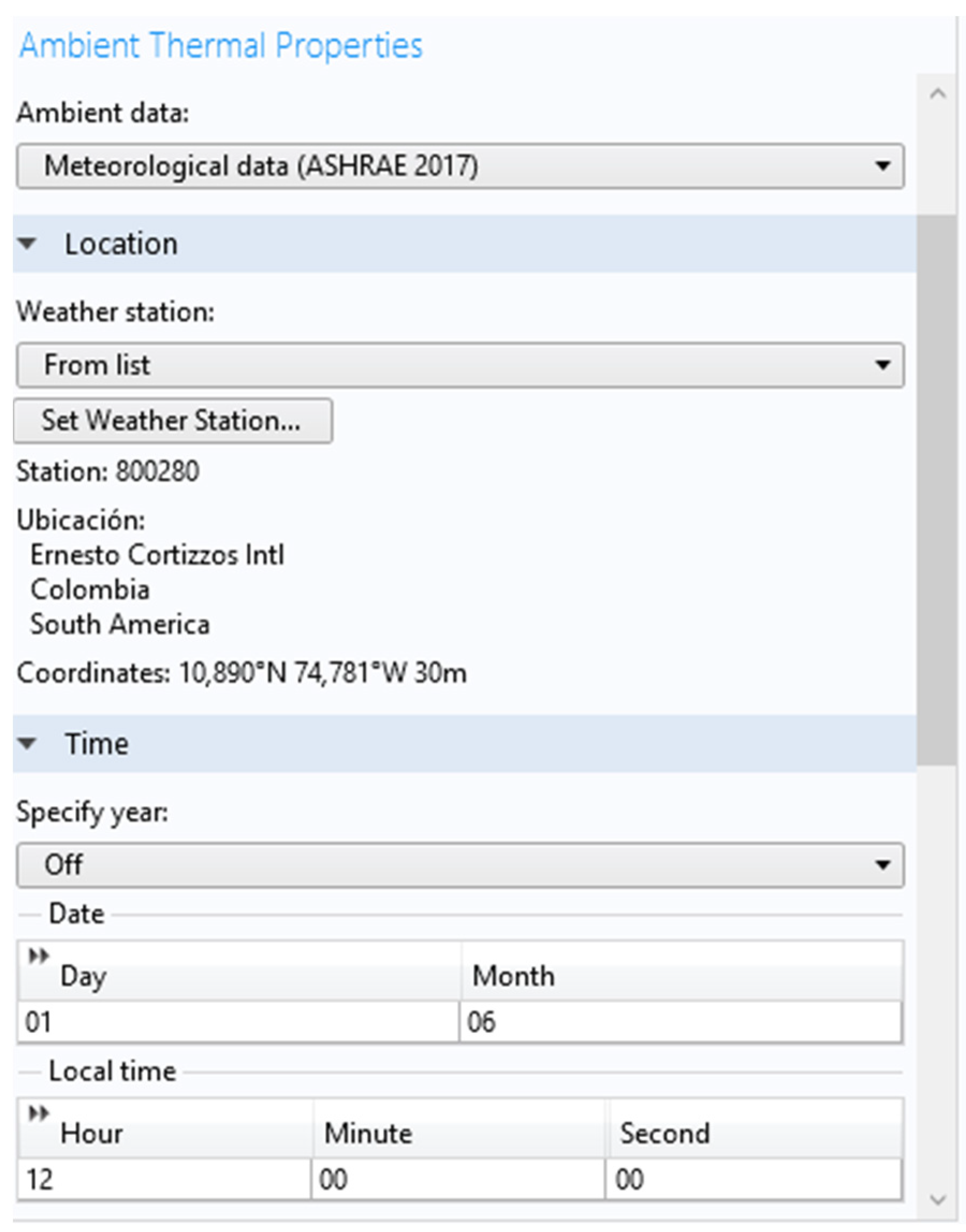
2. Modeling and Computational Details

This section presents the modeling and meshing process of the PV panel for the three cooling methods, as well as the physical processes considered in the investigation. The simulations of the passive, active, and hybrid panels were implemented with the COMSOL Multiphysics software. This software was used because it has an intuitive interface characterized by ease of use and flexibility, which allows the modeling of complex physical problems quickly and accurately. Thus, it was possible to model the phenomena of heat transfer, turbulent flow, radiation in participating media, and the dynamics of water in the solar panels.

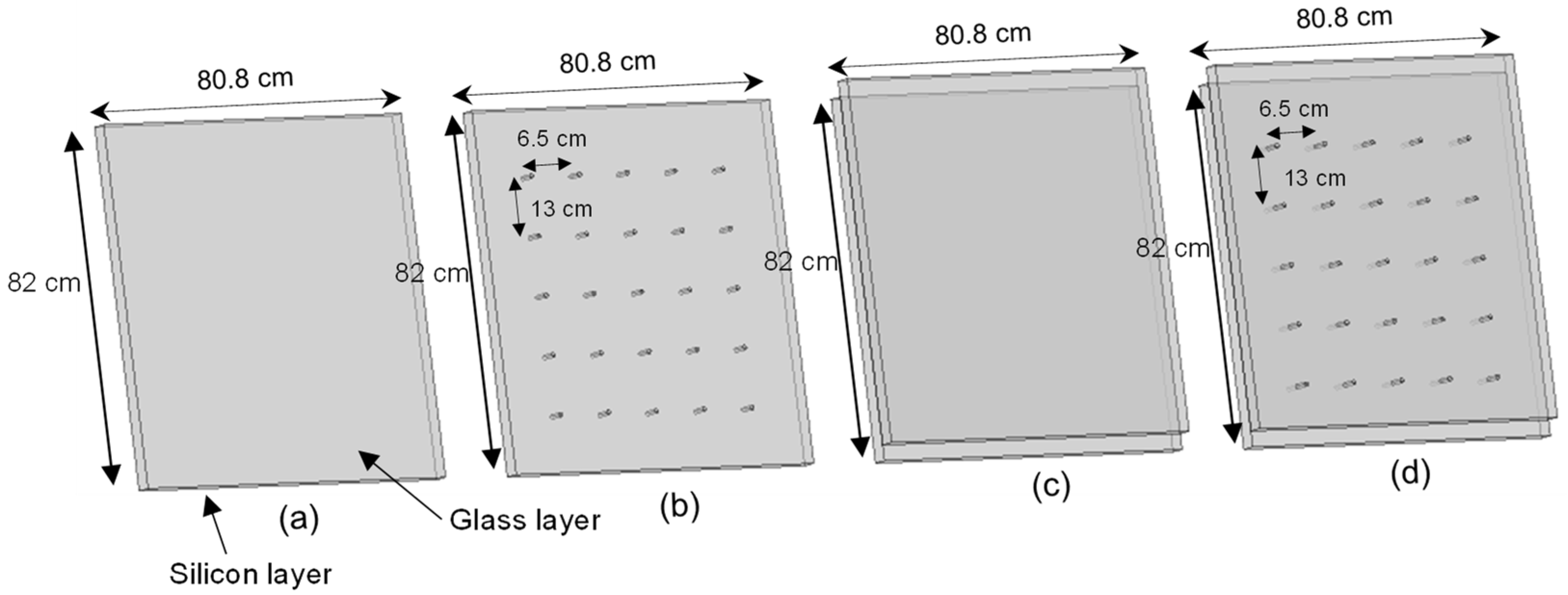
2.1. Modeling of the PV Panel

Figure 1 shows the geometric diagrams of the PV panels modeled for the investigation. The standard PV panel, PV panel with perforations (passive), PV panel with water (active), and hybrid PV panel (passive and active) are presented. The models were implemented with the 3D figure design method of the COMSOL Multiphysics software, for which a geometric figure is defined—in this case a parallelepiped—with the required dimensions.

Thus, the geometry of the PV panel is a rectangle with dimensions of 82 cm × 80.8 cm and a thickness of 0.6 cm. The thickness is divided into a 0.4 cm silicon layer and a 0.2 cm glass layer.

Table 1. Specifications of the panel used in the simulations (SC Origin, SPM100-M).

Specifications	Value
Type	Monocrystalline
Maximum power	100 W
Maximum power voltage	18.75 V
Maximum power current	5.34 A
Open-circuit voltage	22.53 V
Short-circuit current	5.70 A
Temperature power coefficient	−0.45%/°C
Dimensions	820 × 808 × 35 mm

shows the technical specifications of the 100 W panel used.

Table 2. Physical properties of materials used in the simulation.

Properties	Silicon	Water	Air	Units
Density	2329	1000	1.28	kg/m3
Thermal conductivity	130	0.58	0.02	W/(m × K)
Surface emissivity	0.9	0.95	1.012	-
Constant pressure heat capacity	700	4180	-	J/(kg × K)
Thermal expansion coefficient	2.6 × 10−6	-	-	1/K
Relative permittivity	11.7	-	-	-
Dynamic viscosity	-	0.001	0.0000174	Pa × s

shows the physical properties of the materials used in the simulation.

In the case of the perforated panel, the same structure as for the standard panel was modeled but perforating several parts of its area with a matrix built based on cylinders, which were defined with a circumference and a separation distance between holes of 6.5 cm in width and 13 cm in length. The diameter implemented for the cylinders is 1 cm. For the active method, water was sprayed on the surface of the solar panel, to act as a heat sink. For the simulation of the hybrid panel, an additional geometry of equal dimension to the standard panel was considered, but using water as a material, and then superimposing the two geometries to study the dissipation effect that water could cause. After that, using a simple Boolean operation, that matrix was subtracted from the geometry of the PV panel (parallelepiped).

A physics-controlled meshing adjustment tool was used to define the geometry of the PV panels. Thus, the COMSOL software chooses the most pertinent mesh depending on the study to be carried out. Thus, we implement a mesh with a tetrahedral meshing algorithm, and a minimum element size of 0.06 m and a maximum of 0.48 m (

Table 3. Mesh parameters.

Parameter	Value
Maximum element size	0.48 (m)
Minimum element size	0.06 (m)
Maximum element growth rate	1.45
Curvature factor	0.5
Resolution of narrow regions	0.6

). After choosing a fine mesh resolution, the results shown in Figure 2 were obtained. The panel is enclosed in a computational domain with dimensions of 4 m × 4 m × 2 m, which allows observing the behavior of the wind around the PV panel and graphing the flow only in the contours where it collides with the panel. Both the PV panel and the computational domain are meshed (Figure 2), and the specifications obtained are shown in

Table 4. Specifications of the domains and meshes implemented.

Computational Domain	Domains	Sides	Edges	Points
Standard panel	3	17	32	20
Passive panel	3	117	332	220
Active panel	4	23	44	28
Hybrid panel	4	124	348	232
Mesh Specifications	Domain Elements	Boundary Elements	Edge Elements
Standard panel	1415321	55018	1441
Passive panel	3731403	107882	2931
Active panel	920878	45450	1259
Hybrid panel	3042372	135418	3329

.

Finally, meteorological data used in the simulation were taken from the station located at the Ernesto Cortizzos airport in Colombia (Figure 3). For this, we used the ambient thermal properties interface, which allows modifying parameters such as temperature and simulation date.

2.2. Description of the Physical Processes

Considering the different physical processes that are presented in this research (heat transfer, radiation, fluid dynamics, and power analysis of PV panels), the appropriate modules that provide physical interfaces and tools to model the main physical phenomena were chosen. To find the required solutions, in this work fluid mechanics was combined with numerical methods using three key elements: turbulence modeling, mesh construction, and algorithm development. These three elements can be introduced in the simulation with COMSOL Multiphysics, which leads to finding a relationship of the study variables.

Calculations were performed using the turbulent flow modules, where the RANS (Reynolds-averaged Navier–Stokes) k-ε model was chosen together with the non-isothermal flow multiphysics. The model of heat transfer in solids by radiation was used to study the behavior of the panel.

2.2.1. Heat Transfer

Convection heat transfer was modeled with Newton’s law of cooling (Equation (1)), which is proportional to the difference between the surface temperature $\left(T\right)$ and the fluid temperature $\left(T_{\mathrm{ext}}\right)$. The constant of proportionality, $h$, is called the convective heat transfer coefficient.

$$q_0=h\left(T_{\mathrm{ext}}-T\right)$$

(1)

Equation (2) represents the temperature gradient, which is equal to heat transfer by convection [18].

$$-n·\left(-k\nabla T\right)=h\left(T_{\mathrm{ext}}-T\right)$$

(2)

2.2.2. Surface-to-Surface Radiation

COMSOL incorporates a surface-to-surface radiation interface, which was used to model radiation heat transfer. This interface considers thermal radiation as an energy transfer between boundaries and external heat sources where the medium does not participate in the radiation (radiation in transparent media).

While the surface-to-surface radiation heat transfer interface calculates the temperature field, this physical interface requires it as input to the model. If the medium participates in the radiation (semi-transparent medium), the radiation interface on participating media is used. The radiosity equation, defined in the limits where surface-to-surface radiation is enabled, corresponds to the equation of the radiosity method [19].

2.2.3. Turbulent Fluid Flow

To describe the phenomenon of mass and momentum transport, the Reynolds-averaged Navier–Stokes equations were implemented. These equations include unknown terms that are modeled through the closing equations that are based on an approximation to the viscous nature of the problem [20]. For a non-compressible Newtonian flow, the Navier-Stokes Equations take the form:

$$\rho \nabla ·u=0$$

(3)

$$\rho \frac{\partial u}{\partial t}+\rho \left(u·\nabla \right)u=\nabla ·\left[-pI+\mu \left(\nabla u+{\left(\nabla u\right)}^T\right)\right]+F$$

(4)

where: $\rho$: density; $p$: pressure; $u$: fluid velocity; $\mu$: dynamic viscosity; $F$: volumetric forces that can affect movement.

2.2.4. RANS $k-\epsilon$ Turbulence Model

To model the dynamics of the water on the solar panels, the $k-\epsilon$ turbulence model was implemented. This model is the most used for the study of fluids in industrial applications due to its robustness and low computational cost and consists of solving two equations: for the turbulent kinetic energy transport $k$ (which determines the energy in the turbulence) and for the dissipation rate of the turbulent kinetic energy $\epsilon$ (which determines the scale of the turbulence) [21]. With the values of $k$ and $\epsilon$, it is possible to obtain ${\mu }_T$ (Equation (5)).

$${\mu }_T=\rho C_{\mu }\frac{k^2}{\epsilon }$$

(5)

where $C_{\mu }$ is a constant. The transport equation for turbulent kinetic energy is:

$$\rho \frac{\partial k}{\partial t}+\rho \left(u·\nabla \right)k=\nabla ·\left[\left(\mu +\frac{{\mu }_T}{{\sigma }_k}\right)\nabla k\right]+P_k-\rho \epsilon$$

(6)

$$P_k={\mu }_T\left[\nabla u:\left(\nabla u+{\left(\nabla u\right)}^T\right)-\frac{2}{3}{\left(\nabla ·u\right)}^2\right]-\frac{2}{3 }\rho k\nabla ·u$$

(7)

The transport equation for the turbulence dissipation rate is:

$$\rho \frac{\partial \epsilon }{\partial t}+\rho \left(u·\nabla \right)\epsilon =\nabla ·\left[\left(\mu +\frac{{\mu }_T}{{\sigma }_{\epsilon }}\right)\nabla \epsilon \right]+C_{\epsilon 1}\frac{\epsilon }{k}{P}_k-C_{\epsilon 2}\rho \frac{{\epsilon }^2}{k}$$

(8)

2.2.5. Photovoltaic Panel Equation

To obtain the power differences in the modeled PV panels, from the temperature differences obtained with the passive and active cooling methods, the mathematical modeling of the PV panel was performed with the I-V relationship described in Equation (9) [22,23].

$$I\left(V\right)=\frac{I_{x }}{1-e^{-\frac{1}{b}}}\left[1-e^{\frac{V}{b{V}_x }-\frac{1}{b}}\right]$$

(9)

where $V_x$ and $I_x$ are the open-circuit voltage and the short-circuit current for dynamic values of irradiance and temperature and are defined by:

$$V_x=s\frac{E_i}{E_{iN}}{T}_{CV}\left(T-T_N\right)+s\left(V_{\max }\right)-s\left(V_{\max }-V_{\min }\right)e^{\frac{ E_i}{E_{iN}}Ln \frac{V_{\max }-V_{oc}}{V_{\max }-V_{\min }} }$$

(10)

$$I_x=p\frac{E_i}{{\mathrm{E}}_{iN}}\left[I_{sc}+T_{Ci}\left(T-T_N\right)\right]$$

(11)

where $b$ is the constant characteristic of the PV panel; it has no units, and it is the only parameter that must be calculated in this model. $s$: represents the number of panels in series. $p$: represents the number of panels in parallel. $E_i$: is the effective irradiation at which the panel operates. $E_{iN}$: is an irradiation constant of 1000 W/m². $T$: is the operating temperature at which the panel operates. $T_N$: is a temperature constant of 25 °C. $V_{oc}$: is the open-circuit voltage. $I_{sc}$: is the short-circuit current. $V_{\max }-V_{\min }$: are the open-circuit voltage values for irradiation levels less than 200 W/m² and greater than 1200 W/m² with an operating temperature of 25 °C. These values are around $85\%$ of $V_{oc}$ for $V_{\min }$ and $103\%$ of $V_{oc}$ for the case of $V_{\max }$. $T_{Ci}$: is the temperature coefficient of current. $T_{CV}$: is the temperature coefficient of voltage.

Equations (9)–(11) were used for the modeling of the PV panel in Matlab for variable operating conditions in temperature and irradiation. For this, a monocrystalline 100 W PV panel was used (Table 1), with a tolerance of $\pm 3\%$ and the following electrical characteristics for $E_i=1000 \mathrm{W}/{\mathrm{m}}^2$ and T = 25 °C: Short-circuit current ($I_{sc}$) = 5.7 A. Open-circuit voltage ($V_{oc}$) = 22.53 V. Voltage at maximum power point ($V_{\mathrm{pmax}}$) = 18.75 V. Current at maximum power point ($I_{\mathrm{pmax}}$) = 5.34 A. Temperature coefficient of voltage ($T_{CV}$) = −0.35 V/°C. Temperature coefficient of current ($T_{Ci}$) = 0.05 A/°C. Maximum voltage ($V_{\max }$) = 23.21 V. Minimum voltage ($V_{\min }$) = 19.16 V.

In addition to the parameters presented, it is necessary to find the value of b, which is the only parameter that must be calculated. The value of b is in the range of 0.01 to 0.18, therefore, the following approximation can be established [24]:

$$1-e^{\frac{-1}{b}}\approx 1$$

(12)

For $V_x=22.53 \mathrm{V}$, $I_x=5.7\mathrm{A}$, $I=5.34 \mathrm{A}$, and $V=18.75 \mathrm{V}$, the value of $b$ found using Equation (9) is $b=0.06073$.

3. Results and Discussion

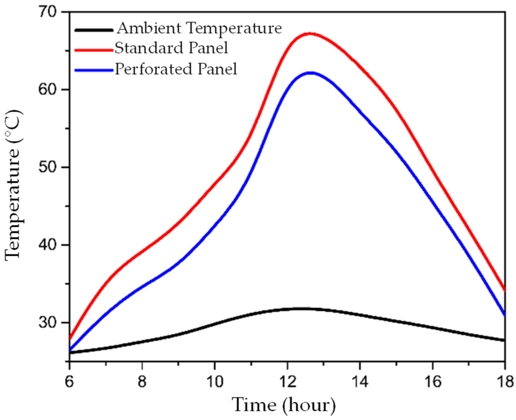
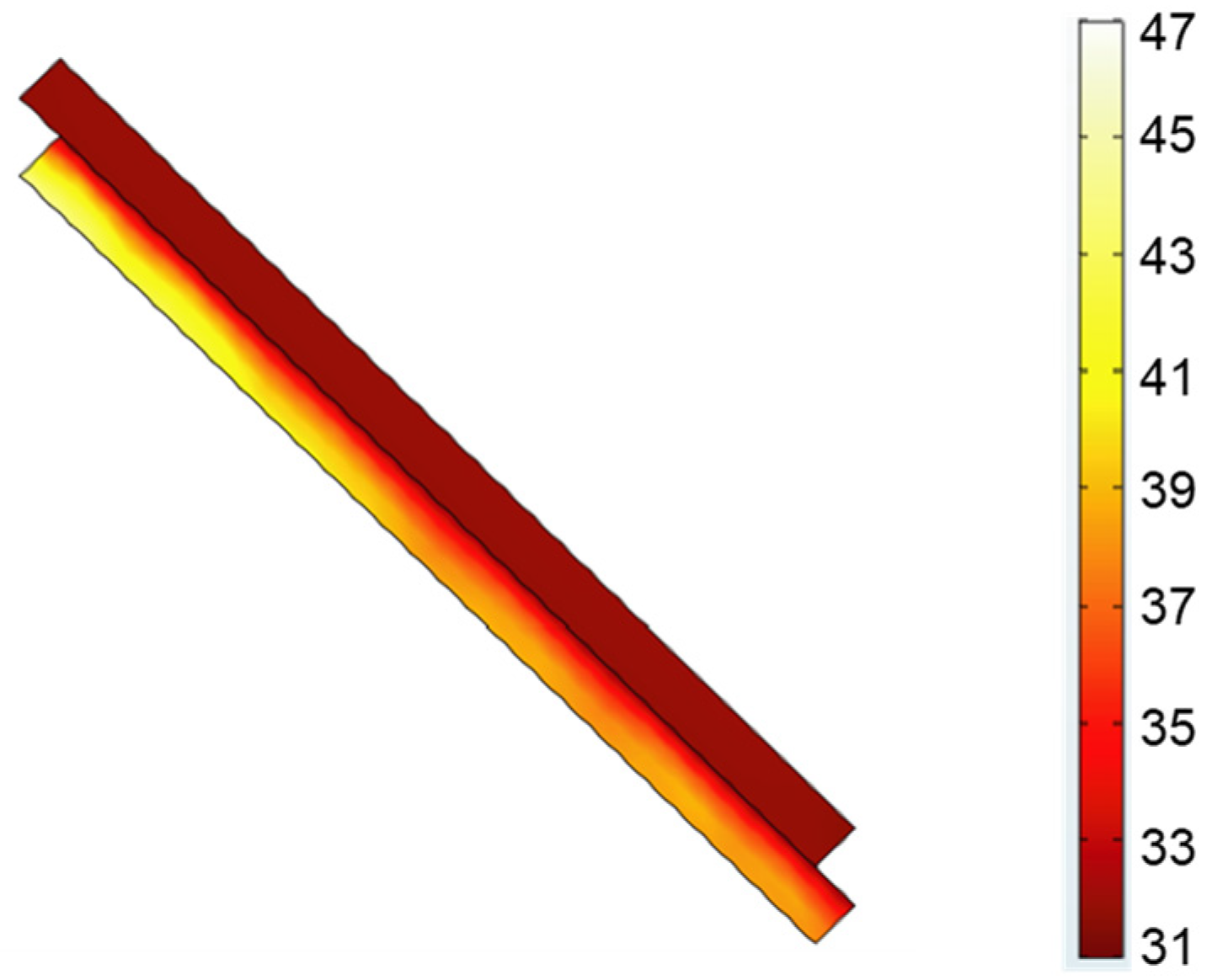
This chapter presents the results obtained by solving the equations described in the previous section, and an analysis of the effects of each cooling method tested is made. To model all the methods, a stationary study considering the unpredictability of turbulent flow was performed.

3.1. Passive Method

In this method, direct holes were made in the PV panel, as described in the modeling section. To analyze the behavior of the PV panel, the physics modules of turbulent fluid flow, heat transfer, and radiation were used. Figure 4 and Figure 5, and

Table 5. Temperature values of the PV panels for different hours of the day (standard—perforated).

Time	Amb. T. (°C)	Std. Panel (°C)	Perf. Panel (°C)	Diff. Std.—Perf. Panel (°C)
6:00	26.12	27.90	26.45	1.45
7:00	26.65	35.77	31.32	4.45
8:00	27.55	39.15	34.75	4.40
9:00	28.36	42.44	37.23	5.21
10:00	29.85	47.97	42.41	5.56
11:00	31.16	52.62	47.92	4.70
12:00	31.86	67.70	62.36	5.34
13:00	31.78	67.34	62.60	4.74
14:00	30.98	63.07	57.01	6.06
15:00	30.17	57.94	52.33	5.61
16:00	29.37	49.41	45.50	3.91
17:00	28.45	42.08	38.80	3.28
18:00	27.69	34.14	30.90	3.24
Prom.	29.23	48.27	43.81	4.46

show the results obtained for the temperature variation, which are compared with the temperature behavior of the standard PV panel.

Figure 4 shows a diagram of the temperature distribution in the cell, for standard and perforated PV panels; and Table 5 shows the different values of temperature reached by the standard panel (Stand. PV Panel Temp.), the perforated panel (Perf. PV Panel Temp.) and their difference (Diff. Stand. PV Panel—Perf. PV Panel), considering a variation in ambient temperature (Amb. Temp.).

Comparing the temperature values presented in Table 5, an average reduction of 4.46 °C can be observed for the perforated module compared to the standard module, with a minimum variation of 1.45 °C, and a maximum of 6.06 °C.

Figure 6 shows the behavior of the wind as it passes through the solar panels. More turbulence flow can be seen for the perforated panel compared to the standard panel. In this way, the operating temperature of the perforated panel is reduced, since any turbulent fluid works as a passive diffuser. This situation is confirmed with the results obtained for the boundary layer of the panels (Figure 7). In this figure, it is observed that the difference in the shape of layers is caused by the holes in the perforated panel.

Finally,

Table 6. Power values of the PV panels for different hours of the day (standard—perforated).

Time	Std. Panel (W)	Perf. Panel (W)	Diff. Std.—Perf. Panel (W)
10:00	67.61	71.29	3.68
11:00	63.98	67.61	3.63
12:00	50.16	55.71	5.55
13:00	50.76	55.37	4.61
14:00	54.80	60.44	5.64
15:00	59.65	64.41	4.76
Prom.	57.83	62.47	4.65

shows the results in the output power of the PV panels modeled in this section, for which the mathematical model of the PV panel implemented in Matlab was used. These data were taken during sunny hours when the panel was exposed to the greatest radiation, from 10 a.m. to 3 p.m. With the perforated panel, a higher power output was achieved due to the improvements obtained in the operating temperature in relation to the standard panel.

3.2. Active Method

As an active cooling method, water was sprayed on the surface of the solar panel, to act as a heat sink. For the analysis of the cooling effect with water, the radiation and heat transfer modules of COMSOL were used. Figure 8, Figure 9 and Figure 10, and

Table 7. Temperature values of the PV panels for different hours of the day (standard—active).

Time	Amb. T. (°C)	Std. Panel (°C)	Act. Panel Wat. Amb. T. (°C)	Act. Panel Wat. 10° (°C)	Act. Panel Wat. 5° (°C)	Diff. Std.—Act. Panel Wat. Amb. T. (°C)
6:00	26.12	27.90	26.04	10.62	6.15	1.86
7:00	26.65	35.77	26.62	10.77	7.08	9.15
8:00	27.55	39.15	28.20	11.56	7.75	10.95
9:00	28.36	42.44	29.89	11.87	6.21	12.55
10:00	29.85	47.97	33.11	12.98	8.51	14.86
11:00	31.16	52.62	36.05	12.36	8.64	16.57
12:00	31.86	66.21	37.83	13.52	8.64	28.38
13:00	31.78	67.34	39.03	13.75	8.65	28.31
14:00	30.98	63.07	38.76	13.72	8.48	24.31
15:00	30.17	57.94	37.45	12.22	8.20	20.49
16:00	29.37	49.41	35.49	12.34	7.71	13.92
17:00	28.45	42.08	32.94	11.86	6.96	9.14
18:00	27.69	34.14	29.46	10.93	6.02	4.68
Prom.	29.23	48.16	33.14	12.19	7.62	15.01

show the results obtained for the temperature variation, and it is compared with the temperature behavior of the standard panel.

Table 7 shows the temperatures of the standard solar panel (Std. Panel) and the active panel with water at different times of the day, considering the variation in ambient temperature and different water temperatures at the time of spraying: ambient temperature (Act. Panel Wat. Amb. T.), 10 °C (Act. Panel Wat. 10 °) and 5 °C (Act. Panel Wat. 5 °). The last column shows the temperature difference between the standard panel and the panel with water at ambient temperature (Diff. Std.—Act. Panel Wat. Amb. T.).

Table 7 shows an average reduction of 15 °C in the temperature of the active panel sprayed with water at ambient temperature compared to the standard panel without water, with a minimum variation of 1.86 °C, and a maximum of 28.38 °C. It can also be observed that by lowering the water temperature by any conventional method, it is possible to achieve a greater reduction in the panel temperature, further improving its efficiency. In this scenario, the cases of water at temperatures of 10 °C and 5 °C were considered and a greater reduction in temperature can be observed compared to the panel with water at ambient temperature.

Finally, in

Table 8. Power values of the PV panels for different hours of the day (standard—active).

Time	Std. Panel (W)	Act. Panel Wat. Amb. T. (W)	Act. Panel Wat. 10° (W)	Act. Panel Wat. 5° (W)	Diff. Std.—Act. Panel Wat. Amb. T. (W)
10:00	67.61	76.00	81.49	81.65	8.39
11:00	63.98	74.68	81.42	81.65	10.70
12:00	50.16	73.79	81.38	81.65	23.63
13:00	50.76	73.05	81.33	81.65	22.29
14:00	54.80	73.25	81.35	81.65	18.45
15:00	59.65	73.94	81.49	81.65	14.29
Prom.	57.83	74.12	81.41	81.65	16.29

, it can be seen how this system substantially improves the power of the panel compared to the results obtained with the perforated panel (Table 6). In addition, these results reflect that there is a point in which it does not matter how much the temperature decreases, since there will be no significant contribution to the increase in power.

3.3. Hybrid Method

To analyze the effect that the two methods applied simultaneously on the solar panel can produce, a perforated panel with a layer of water on it (hybrid panel) was simulated. For the performance analysis, the fluid flow, heat transfer, and radiation physics modules were used. Figure 11 and Figure 12, and

Table 9. Temperature values of the PV panels for different hours of the day (standard—hybrid).

Time	Amb. T. (°C)	Std. Panel (°C)	Hyb. Panel Wat. Amb. T. (°C)	Diff. Std.—Hyb. Panel Wat. Amb. T. (°C)
6:00	26.12	27.90	25.17	2.73
7:00	26.65	35.77	25.97	9.80
8:00	27.55	39.15	28.10	11.05
9:00	28.36	42.44	29.67	12.77
10:00	29.85	47.97	30.28	17.69
11:00	31.16	52.62	33.50	19.12
12:00	31.86	66.21	34.51	31.70
13:00	31.78	67.34	35.15	32.19
14:00	30.98	63.07	34.83	28.24
15:00	30.17	57.94	34.31	23.63
16:00	29.37	49.41	32.11	17.30
17:00	28.45	42.08	30.90	11.18
18:00	27.69	34.14	27.48	6.66
Prom.	29.23	48.16	30.92	17.24

show the results obtained for the temperature variation in this case, which are compared with the temperature performance of the standard panel.

Table 9 shows the different values of the temperature reached by the standard panel (Std. Panel) and the hybrid panel at different times of the day, considering the variation in ambient temperature (Hyb. Panel Wat. Amb. T.). The final column shows the temperature difference between the standard panel and the hybrid panel with water at ambient temperature (Diff. Std.—Hyb. Panel Wat. Amb. T.).

As can be corroborated from the data recorded in Table 9, the combined passive and active cooling methods (hybrid panel) produce a drop in temperature compared to the standard panel. It is highlighted that this decrease is on average 2.2 °C less than the decrease caused by the active method (Table 8).

As in the previous cases, in this system, the data obtained by the mathematical model of the panel power were obtained (See

Table 10. Power values of the PV panels for different hours of the day (standard—hybrid).

Time	Std. Panel (W)	Hyb. Panel Wat. Amb. T. (W)	Diff. Hyb.—Act. Panel Wat. Amb. T. (W)
10:00	67.61	77.24	9.63
11:00	63.98	76.04	12.06
12:00	50.16	75.38	25.22
13:00	50.76	75.12	24.36
14:00	54.80	75.23	20.43
15:00	59.65	75.46	15.81
Prom.	57.83	75.75	17.92

).

3.4. Comparison of the Implemented Methods

When a comparison is performed between the three implemented alternatives (perforated panel, active panel, and hybrid panel), it was possible to establish that the greatest decrease in temperature is achieved with the hybrid solar panel. In absolute values, with the hybrid panel, an average decrease of 17.24 °C was obtained compared to 15.01 °C for the active panel and 4.46 °C for the perforated panel (See

Table 11. Temperature differences between the solar panels evaluated.

Time	Diff. Std.—Perf. Panel (°C)	Diff. Std.—Act. Panel Wat. Amb. T. (°C)	Diff. Std.—Hyb. Panel Wat. Amb. T. (°C)
6:00	1.45	1.86	2.73
7:00	4.45	9.15	9.80
8:00	4.40	10.95	11.05
9:00	5.21	12.55	12.77
10:00	5.56	14.86	17.69
11:00	4.70	16.57	19.12
12:00	5.34	28.38	31.70
13:00	4.74	28.31	32.19
14:00	6.06	24.31	28.24
15:00	5.61	20.49	23.63
16:00	3.91	13.92	17.30
17:00	3.28	9.14	11.18
18:00	3.24	4.68	6.66
Prom.	4.46	15.01	17.24

). In percentage terms, with the hybrid solar panel, a decrease of 287% in operating temperature was obtained compared to the passive solar panel and 15% compared to the active solar panel.

In terms of the output power of the solar panels, with the decrease in the operating temperature, better results were obtained. Obviously, with the hybrid solar panel higher power was obtained on average (17.92 W) compared to the active solar panel (16.29 W) and the passive solar panel (4.65 W) (

Table 12. Differences between the output power of the solar panels evaluated.

Time	Diff. Std.—Perf. Panel (W)	Diff. Std.—Act. Panel Wat. Amb. T. (W)	Diff. Hyb.—Act. Panel Wat. Amb. T. (W)
10:00	3.68	8.39	9.63
11:00	3.63	10.7	12.06
12:00	5.55	23.63	25.22
13:00	4.61	22.29	24.36
14:00	5.64	18.45	20.43
15:00	4.76	14.29	15.81
Prom.	4.65	16.29	17.92

). In percentage terms, the hybrid panel obtained 286% more power compared to the passive panel and 10% more compared to the active panel.

This situation shows that the hybrid solar panel has better performance in terms of power output. However, it is noteworthy that both the active panel and the passive panel improve the performance of the standard solar panel.

4. Conclusions

Air currents through the solar panel play a very important role for natural (passive) convection models, becoming useful tools for reducing high temperatures due to their turbulent characteristics. The standard k-ε model performed satisfactorily in the COMSOL Multiphysics software when evaluating mass air flow, due to the behavior of the simulations and the computational costs, which is in line with results obtained in previous turbulence analysis studies [25] and passive cooling strategies for solar panels [26].

Regarding the performance of the three evaluated solar panels (passive, active, and hybrid), it could be shown that the hybrid panel presented better performance with a greater decrease in operating temperature and increase in output power. With this method, it was possible to reduce the operating temperature by 17.24 °C on average, while with the active methods, reductions of 15.01 °C and 4.46 °C were obtained, respectively.

It is worth mentioning the decrease in temperature obtained with the passive model and the increase in the output power. Although this model presented lower efficiency by reducing the operating temperature by 4.46 °C and increasing the power by 4.65 W on average, it can be easily applicable in some solar installations. These results were obtained with solar panels modeled with a layer of silicon and one of glass, without considering the support structure [26], in order to reduce computation times.

There remains a gap between laboratory prototypes and industrial applications. The tests performed in this project showed that it is possible to increase the electrical production of a photovoltaic solar panel, however, a cost analysis was not implemented. This is an important factor for the future implementation of practical applications. However, water cooling is still an attractive solution to mitigate the thermal effects in photovoltaic panels. The capacity of this method can be improved if the panel can be cooled with water to temperatures below ambient temperature, but the application of this mechanism will depend on the needs to be required in the installation.

References

1. Kannan, N.; Vakeesan, D. Solar energy for future world—A review. Renew. Sustain. Energy Rev. 2016, 62, 1092–1105. [Google Scholar] [CrossRef]
2. Rauf, A.; Liu, X.; Amin, W.; Ozturk, I.; Rehman, O.U.; Sarwar, S. Energy and ecological sustainability: Challenges and panoramas in belt and road initiative countries. Sustainability 2018, 10, 2743. [Google Scholar] [CrossRef] [Green Version]
3. Robles Algarin, C.; Rodríguez Álvarez, O. An overview of the renewable energy in the World, Latin America and Colombia. Espacios 2018, 39, 1–16. [Google Scholar]
4. Franco, M.A.; Groesser, S.N. A Systematic Literature Review of the Solar Photovoltaic Value Chain for a Circular Economy. Sustainability 2021, 13, 9615. [Google Scholar] [CrossRef]
5. Fouad, M.M.; Shihata, L.A.; Morgan, I. An integrated review of factors influencing the performance of photovoltaic panels. Renew. Sustain. Energy Rev. 2017, 80, 1499–1511. [Google Scholar] [CrossRef]
6. Kasera, S.; Nayak, R.; Bhaduri, S.C. A Review of Performance of Solar Photovoltaic Refrigeration System. Lect. Notes Electr. Eng. 2022, 766, 641–651. [Google Scholar] [CrossRef]
7. Hasanuzzaman, M.; Malek, A.B.M.A.; Islam, M.M.; Pandey, A.K.; Rahim, N.A. Global advancement of cooling technologies for PV systems: A review. Sol. Energy 2016, 137, 25–45. [Google Scholar] [CrossRef]
8. Nizetic, S.; Papadopoulos, A.M.; Giama, E. Comprehensive analysis and general economic-environmental evaluation of cooling techniques for photovoltaic panels, Part I: Passive cooling techniques. Energy Convers. Manag. 2017, 149, 334–354. [Google Scholar] [CrossRef]
9. Kim, J.; Nam, Y. Study on the Cooling Effect of Attached Fins on PV Using CFD Simulation. Energies 2019, 12, 758. [Google Scholar] [CrossRef] [Green Version]
10. AlAmri, F.; AlZohbi, G.; AlZahrani, M.; Aboulebdah, M. Analytical Modeling and Optimization of a Heat Sink Design for Passive Cooling of Solar PV Panel. Sustainability 2021, 13, 3490. [Google Scholar] [CrossRef]
11. Aamir Al-Mabsali, S.; Chaudhry, H.N.; Gul, M.S. Numerical Investigation on Heat Pipe Spanwise Spacing to Determine Optimum Configuration for Passive Cooling of Photovoltaic Panels. Energies 2019, 12, 4635. [Google Scholar] [CrossRef] [Green Version]
12. Kandeal, A.W.; Thakur, A.K.; Elkadeem, M.R.; Elmorshedy, M.F.; Ullah, Z.; Sathyamurthy, R.; Sharshir, S.W. Photovoltaics performance improvement using different cooling methodologies: A state-of-art review. J. Clean. Prod. 2020, 273, 122772. [Google Scholar] [CrossRef]
13. Maleki, A.; Haghighi, A.; El Haj Assad, M.; Mahariq, I.; Alhuyi Nazari, M. A review on the approaches employed for cooling PV cells. Sol. Energy 2020, 209, 170–185. [Google Scholar] [CrossRef]
14. Osma-Pinto, G.; Ordóñez-Plata, G. Dynamic thermal modelling for the prediction of the operating temperature of a PV panel with an integrated cooling system. Renew. Energy 2020, 152, 1041–1054. [Google Scholar] [CrossRef]
15. Sharma, S.; Sellami, N.; Tahir, A.A.; Mallick, T.K.; Bhakar, R. Performance Improvement of a CPV System: Experimental Investigation into Passive Cooling with Phase Change Materials. Energies 2021, 14, 3550. [Google Scholar] [CrossRef]
16. Dwivedi, P.; Sudhakar, K.; Soni, A.; Solomin, E.; Kirpichnikova, I. Advanced cooling techniques of P.V. modules: A state of art. Case Stud. Therm. Eng. 2020, 21, 100674. [Google Scholar] [CrossRef]
17. COMSOL Multiphysics. Available online: www.comsol.com (accessed on 9 September 2021).
18. Lienhard, J.H., IV. A Heat Transfer Textbook, 5th ed.; Dover Publications, Inc.: New York, NY, USA, 2019; pp. 49–78. [Google Scholar]
19. Surface to Surface Radiation Benchmarks. Available online: https://www.comsol.com/paper/surface-to-surface-radiation-benchmarks-35611 (accessed on 9 September 2021).
20. Bernard, P.S. Turbulent Fluid Flow, 1st ed.; John Wiley & Sons Ltd.: Hoboken, NJ, USA, 2019; pp. 1–65. [Google Scholar]
21. Kajishima, T.; Taira, K. Computational Fluid Dynamics: Incompressible Turbulent Flows, 1st ed.; Springer: Cham, Switzerland, 2017; pp. 207–263. [Google Scholar]
22. Viloria-Porto, J.; Robles-Algarín, C.; Restrepo-Leal, D. A Novel Approach for an MPPT Controller Based on the ADALINE Network Trained with the RTRL Algorithm. Energies 2018, 11, 3407. [Google Scholar] [CrossRef] [Green Version]
23. Robles Algarín, C.; Sevilla Hernández, D.; Restrepo Leal, D. A Low-Cost Maximum Power Point Tracking System Based on Neural Network Inverse Model Controller. Electronics 2018, 7, 4. [Google Scholar] [CrossRef] [Green Version]
24. Robles Algarín, C.; Taborda Giraldo, J.; Rodríguez Álvarez, O. Fuzzy Logic Based MPPT Controller for a PV System. Energies 2017, 10, 2036. [Google Scholar] [CrossRef] [Green Version]
25. Vera, S.; Cortés, M.; Rao, J.; Fazio, P.; Bustamante, W. Testing turbulence models to predict interzonal mass airflows through a stairwell opening for both natural and mixed convection flows in buildings. Rev. Ing. Construcción 2015, 30, 2. [Google Scholar] [CrossRef] [Green Version]
26. Abd-Elhady, M.S.; Serag, Z.; Kandil, H.A. An innovative solution to the overheating problem of PV panels. Energy Convers. Manag. 2018, 157, 452–459. [Google Scholar] [CrossRef]
Figure 1. Schematic of the modeled PV panels. (a) Standard PV panel; (b) PV panel with perforations (passive); (c) PV panel with water (active); (d) hybrid PV panel (passive and active).
Applsci 11 11370 g001
Figure 2. Meshing the geometry of the PV panels.
Applsci 11 11370 g002
Figure 3. Comsol interface for configuring ambient thermal properties.
Applsci 11 11370 g003
Figure 4. Temperature distribution for the PV panels in °C: (a) standard; (b) perforated.
Applsci 11 11370 g004
Figure 5. Temperature of the PV panels for different hours of the day: standard (red), perforated (blue) and ambient temperature (black).
Applsci 11 11370 g005
Figure 6. Wind speed (m/s) and flow lines on the panels: (a) standard; (b) perforated.
Applsci 11 11370 g006
Figure 7. Boundary layer of the wind in the PV panels. (a) Standard panel in vertical position; (b) standard panel with 45° tilt angle; (c) perforated panel with 45° tilt angle.
Applsci 11 11370 g007
Figure 8. Temperature distribution (°C) in the solar panels. (a) Standard; (b) active.
Applsci 11 11370 g008
Figure 9. Heat transfer between solar panel and water.
Applsci 11 11370 g009
Figure 10. Temperature of the PV panels for different hours of the day: standard panel (red), panel with water at ambient temperature (blue), ambient temperature (black), panel with water at 10 °C (purple), and panel with water at 5 °C.
Applsci 11 11370 g010
Figure 11. Temperature distribution (°C) in the solar panels. (a) Standard; (b) hybrid.
Applsci 11 11370 g011
Figure 12. Temperature of the PV panels for different hours of the day: standard panel (red), hybrid panel (blue) and ambient temperature (black).
Applsci 11 11370 g012