Adaptive Decision Support System for On-Line Multi-Class Learning and Object Detection

Abstract

A new online multi-class learning algorithm is proposed with three main characteristics. First, in order to make the feature pool fitter for the pattern pool, the adaptive feature pool is proposed to dynamically combine the three general features, Haar-like, Histogram of Oriented Gradient (HOG), and Local Binary Patterns (LBP). Second, the external model is integrated into the proposed model without re-training to enhance the efficacy of the model. Third, a new multi-class learning and updating mechanism are proposed that help to find unsuitable decisions and adjust them automatically. The performance of the proposed model is validated with multi-class detection and online learning system. The proposed model achieves a better score than other non-deep learning algorithms used in public pedestrian and multi-class databases. The multi-class databases contain data for pedestrians, faces, vehicles, motorcycles, bicycles, and aircraft.

1. Introduction

The importance of computer vision-related technology and research is increasing with the increasing efficiency of hardware computing. The main research areas in computer vision are object detection and classification techniques. Accurate detection and quick identification of objects has always been the most important issue in this area. Among all object detection methods, machine learning is one of the most frequently studied. In recent years, there have been many successful applications such as face detection and recognition [1,2], vehicle detection and tracking [3,4,5], and pedestrian detection [6,7,8]. There many single-class offline learning algorithms in machine learning that use massive training data and algorithms to find an approximation function closest to the unknown target function. The most common ones are Adaptive Boosting [9] and Support Vector Machine [10]. These single-class offline learning algorithms usually require a person to collect and classify a large number of positive and negative samples, after which different feature extraction and selection methods are used to find the distinguishable features for the dataset. Finally, these features are combined into a detection model by using a machine learning algorithm. For multiple objects, it is necessary to train several detection models in the same way. Although single-class offline learning has performed well in the field of object detection, substantial training time is necessary for multi-object detection. Thus, it is not recommended to combine several single object models together. As a result, multi-class offline learning is proposed.

Multi-class offline learning has many benefits, both in detection and classification. For example, detection speed and the discrimination of the multi-class offline learning model in classifying several objects usually perform better than the model built by multiple single-class offline learning models, as multi-class offline learning algorithms are obtained by combining or modifying single-class offline learning algorithms in a variety of ways. In addition, the algorithm, developed in this way, adapts to the multi-category classification problem. Some examples of such algorithms are Multi-class Support Vector Machine [11], Joint Boosting [12], and Random Forests [13]. Although these multi-class offline learning algorithms effectively solve the problem of multiple objects classification, people must collect and classify a large number of positive and negative samples in advance, thus requiring more memory space and training time. These problems could mean that the algorithm cannot be trained in real-time with their application in some specific situations. To solve these problems, an online learning algorithm is proposed in this paper.

The online learning algorithm does not need to collect a large number of positive and negative samples in advance; instead, providing data one by one can make it adapt to the scene gradually. As a result, it does not need to learn the classifier at one time from a large number of samples. This not only reduces the training time of the detection model, but also decreases the memory space required. Most of these online learning algorithms evolved from offline learning algorithms. However, some of them also evolved from single-class to multi-class, like offline learning.

Oza and Russell proposed Online Boosting [14], that is an improved online version of Adaptive Boosting [9], which achieves the effect of boosting by simulating the number of times the data are sampled. Grabner and Bischof proposed another Online Boosting method [15,16], which simulates Adaptive Boosting [9] but executes in a single-step method. It mainly selects the better classifier from the selector and combines these classifiers into one strong classifier. It replaces the weak classifier in the selector according to the adaption degree of samples to update the model. In addition to these improved online learning algorithms inspired by the offline learning algorithm, other algorithms were also proposed to combine with these online learning algorithms, e.g., On-line Conservative Learning, which was proposed by Roth, Peter M. [17,18]. In this algorithm, two models are compared, and the higher confidence sample is taken to automatically update the model. It achieves the goal of complete automatic learning and does not need people to label samples. Saffari [19] proposed On-line Random Forests, which can be applied in multi-class object detection. It trains each Decision Tree by simulating the number of times the data are sampled, without using Pruning. This is an improved version of Random Forest [13].

However, certain problems remain in the existing online learning algorithms. For example, online learning algorithm is an algorithm for general objects, so there is a huge influence on detection accuracy and learning speed depending on how suitable features are selected for these samples [20,21]. The online learning algorithms [14,15,16], use a single feature during learning. If they use a feature that does not detect a certain object well, for example, using a Haar-like feature [22] to detect a ball-shaped object or LBP [23] to detect a smooth object, the performance suffers. In particular, multi-class classification has this problem because a single feature has insufficient distinguishing ability to distinguish several objects at the same time. Therefore, if we can dynamically allocate the type of feature according to the pattern pool, the problem would be solved. In addition, there are some online learning algorithms such as Online Random Forest [19] whose models are irreversible as soon as the decision has been made. As a result, if the algorithm makes a false decision, the final performance of the detection model declines. At this time, if we can adjust the model thoroughly and correct the false decision, the detection model is able to perform well again. In addition, the classification result would also be bad if the feature that is used cannot effectively classify certain special samples. Most of the existing online learning algorithms, [14,15,16] and so on, have this problem. A good solution would be to combine these learning algorithms with an external model according to the status of the model after learning to increase the detection performance of the model. Finally, since the sample of online learning is a one-by-one input, it would also be a challenge to preserve the better distinguished sample. Online Conservative Learning [17,18] chooses the sample which confidence as the updating sample is higher to solve this problem. With this approach, however, we cannot determine the more representative sample. 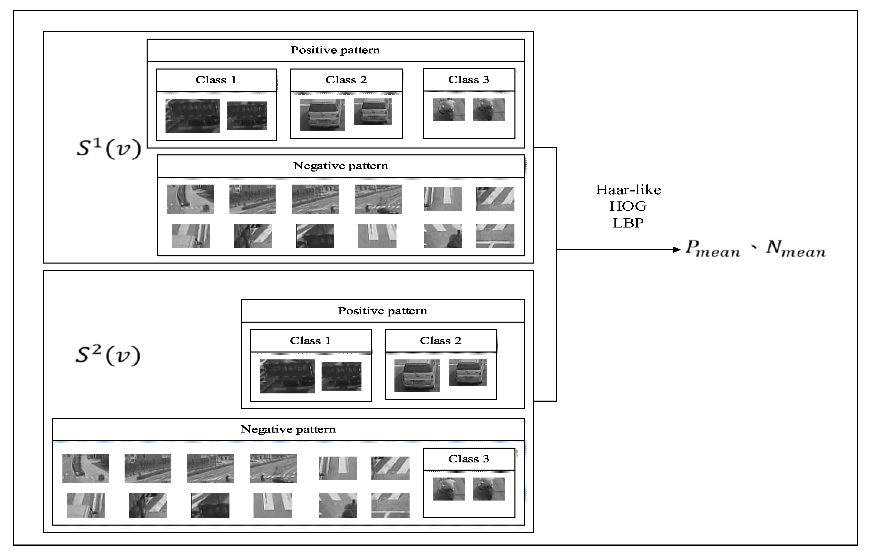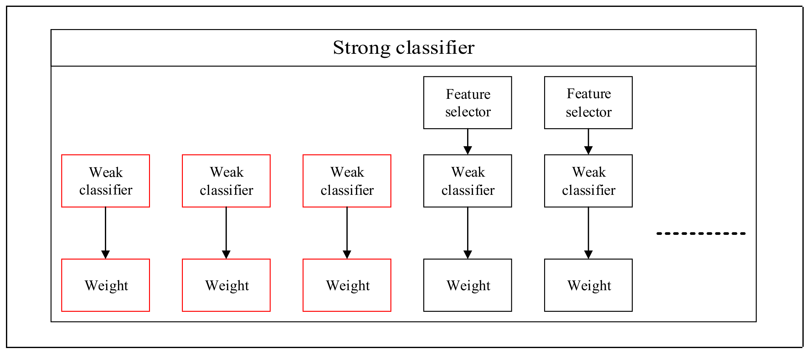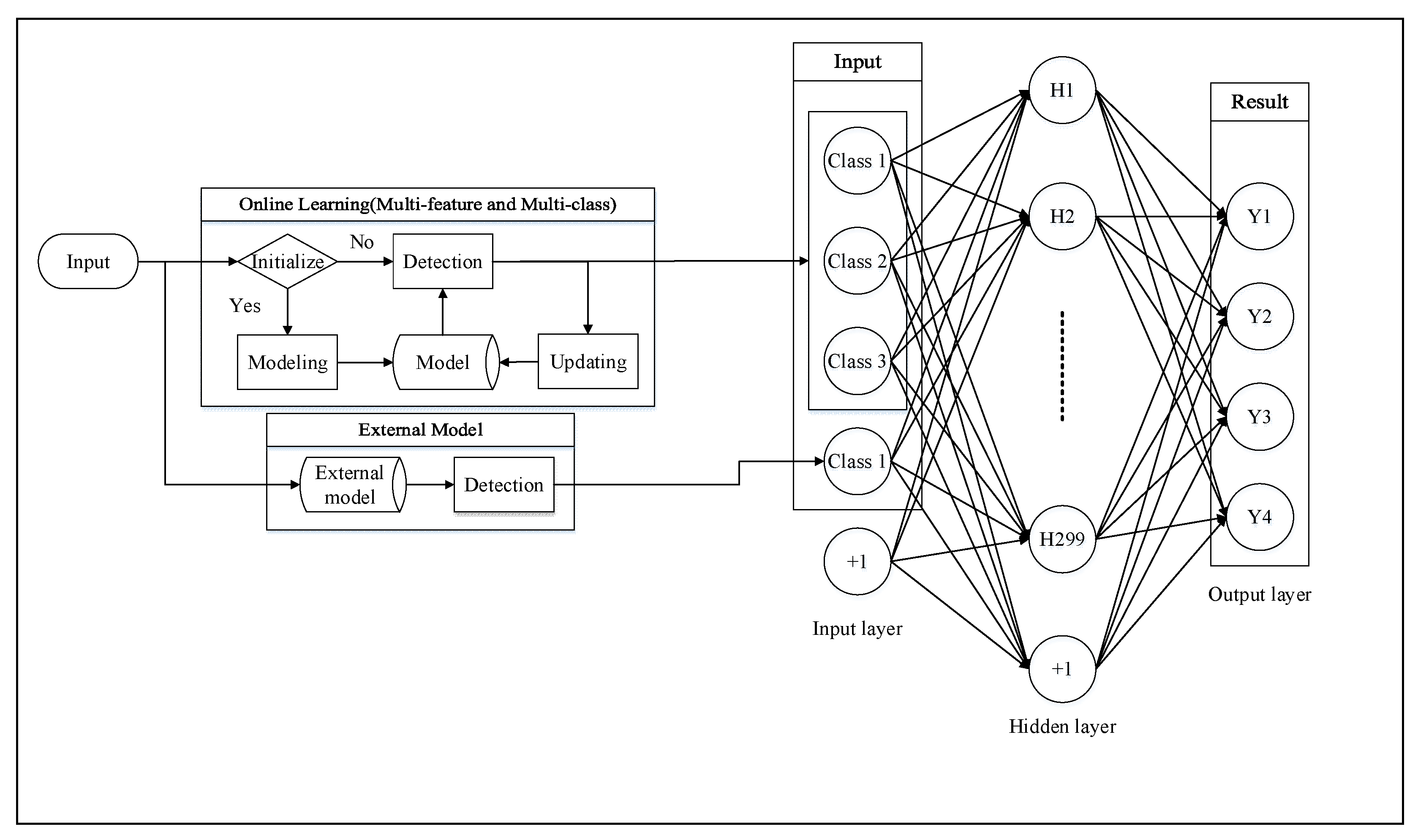Therefore, On-line Learning with Adaptive Model [24] proposes a solution to sample storage and replacement. This method derives the more representative samples by calculating the importance and combining similar samples. For these reasons, this paper proposes an online multi-class learning and detection system that can dynamically allocate features based on samples and can combine with external models based on the learning effect to increase the performance of the model. Therefore, the proposed model not only uses the concept of the sharing feature in Joint Boosting classifier [12] to build the model, but also uses the feature selector in Online Boosting algorithm [15,16] to update and select features that are distinguished better. Then, we used Back Propagation Neural Network [25] to combine it with the external model. 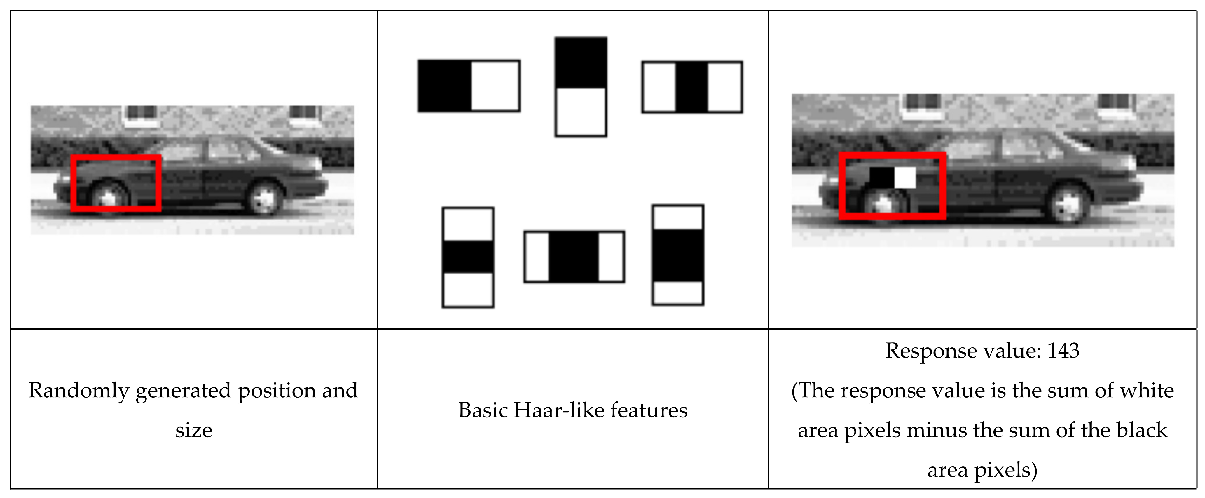In the pattern pool, the proposed model adopts the same method in On-line Learning with Adaptive Model [24] to make an update. 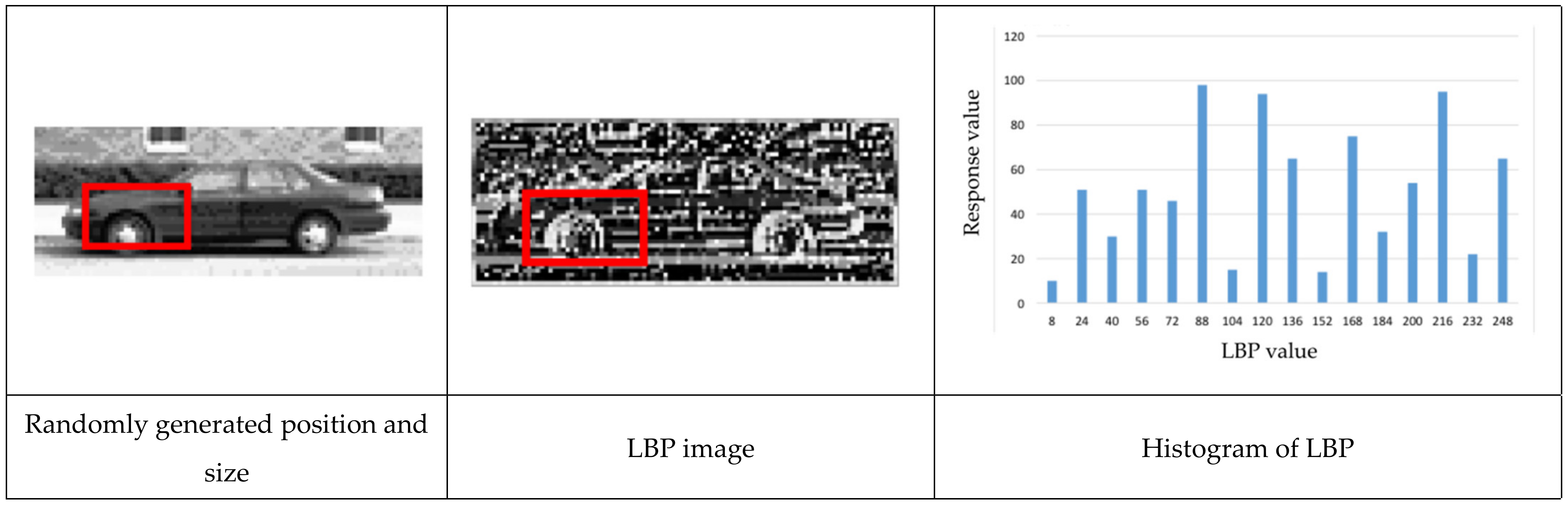In the feature part, the proposed model uses Haar-like [22], Histogram of Oriented Gradient (HOG) [26], and Local Binary Patterns (LBP) [23]. Except for simplifying the last two features so that it can use Integral image [27] to speed up the model, we also proposed an algorithm to dynamically allocate and replace features according to the learning samples. Finally, we proposed a new updating method by combining the Joint Boosting Classifier [12] with the Online Boosting [15,16]. The system is able to adjust the model according to all pattern pools so that it is not affected by previous false decisions.

2. Proposed System

The proposed system flowchart is shown in Figure 1. In the Modeling part, we labelled some target patterns in the input image and collected positive and negative pattern pools from these input images. Then, according to the aspect ratio of the target patterns, we generated the Haar-like [22], HOG [26], and LBP [23] initial feature pools. After that, we determine the applicability of a feature to the patterns by calculating the positive and negative average response value. Further, the adaptive feature pool could be formed by dynamically selecting different proportions of Haar-like, HOG, and LBP features from the initial feature pools. Finally, weak classifiers, which distinguishing abilities are stronger, were chosen to compose a strong classifier. The model is built by these multiple strong classifiers, trained by each class. After the model is built, we set up multiple feature selectors in each strong classifier to speed up the updating of the model. The selector included the feature selected from the adaptive feature pool. In the detection part, the model calculates the score of each class and decides the classification result according to these scores. In the updating part, as the input of the image, model detection is performed and then the misclassified patterns are updated in the pattern pool. We selected the weak classifier that had better distinguishing ability from all the candidate features in each feature selector to replace the weak classifier that had less distinguishing ability in the new pattern pool than the strong classifier. Then, we replaced and updated the candidate features that had less distinguishing ability from the feature selector. Finally, new features were generated to replace the features that were not applicable anymore. In this way, we could dynamically adjust the model. The learned model can also use a neural network [25] to combine with an external model for enhancement and expansion.

2.1. Modeling

This section will introduce how to build the object detection model. It mainly includes feature selection and classifier construction.

2.1.1. Pattern Pool Initialization

For each different class detection target, the user needs to label at least one pattern. The system decides the aspect ratio and scaling range of detection window according to this pattern and generates a positive and negative pattern pool for the algorithm to learn. Figure 2 is an illustration of labeling the detection targets. The generation of patterns in a positive and negative pattern pool is decided by the overlapping area of the labeled target and sliding window in each input image, as given in (1)

$$Overlap=\frac{area\left(B_{sample}\cap B_{sliding}\right)}{area\left(B_{sample}\cup B_{sliding}\right)}$$

(1)

The size of the sliding window starts from the minimum labeled target and zooms in equal magnification (1.2 in this research) until the size reaches the largest labeled size. The scanning stride is the short side of the sliding window times the fixed magnification (0.1 in this research) to scan through the whole image. Then, the pattern is generated by calculating the overlapping area. We used the same setting as in On-line Learning with Adaptive Model [24]. If the overlapping area is larger than 0.875, it is viewed as a positive pattern, as shown in Figure 3. Note that the overlap area of the positive sample is set to be less than 0.8, and it is not conducive to the selection of initial features. It will also affect the correctness of the object classification. If the overlapping area is less than 0.3, it is viewed as a negative pattern, as shown in Figure 4.

The above steps are completed in the first labeled frame. As for the other labeled frames, the positive patterns are also chosen using the above steps. The negative patterns are taken where the overlapping area is between 0 and 0.3. At the same time, if the overlapping area between the positive pattern’s position of the first labeled frame and the positive pattern of this frame is 0, this area would also be seen as a negative pattern to make up the background occluded by the positive pattern in the first labeled frame, as shown in Figure 5.

2.1.2. Generation of Adaptive Feature Pool

Since, the focus of this paper is an online detection system for multiple objects, a single feature is insufficient. Therefore, we adopted and combined three different feature descriptors that have good performance in different kinds of images. There are Haar-like features, which can detect the change in grey level, HOG features, which are good at analyzing gradient direction, and LBP features, which can analyze the image texture. In the initializing part, the proposed system generates 1000 Haar-like, HOG, and LBP initial features each according to the aspect ratio of the labeled target patterns. We adopted six kinds of basic Haar-like features with random scales and positions. Figure 6 shows the basic Haar-like features that are used and the process of feature extraction. To use HOG and LBP features, we simplify them to increase the processing speed. The simplified method is similar to a Haar-like feature. After randomly generating the position and size of a rectangle in the training pattern, HOG calculates the statistics of the gradient value in this rectangle to derive a nine-dimensional histogram for feature extraction, as shown in Figure 7. LBP calculates the statistics of the LBP in this rectangle to derive a sixteen-dimensional histogram for feature extraction, as shown in Figure 8.

After calculating the initial features, we used the difference between the average feature response value of the positive patterns and the negative patterns ($P_{mean}$ and $N_{mean}$) as the distinguishing ability of a feature from the existing patterns. We selected 1000 Haar-like, HOG, and LBP initial features randomly in this way. The total number of features of 1000 can be adjusted according to the calculation performance. In the experiment, using 1000 initial features for selection and replacement, all can achieve real-time calculations and maintain sufficient detection results. The number of dynamically selected features for each type are shown in (2)–(4). Finally, we adopted these initial features to compose the adaptive feature pool.

Number of dynamic Haar-like features:

$$\frac{\left|Haar{P}_{mean}-Haar{N}_{mean}\right|\times 1000}{\left|Haar{P}_{mean}-Haar{N}_{mean}\right|+\left|HOG{P}_{mean}-HOG{N}_{mean}\right|+\left|LBP{P}_{mean}-LBP{N}_{mean}\right|}$$

(2)

Number of dynamic HOG features:

$$\frac{\left|HOG{P}_{mean}-HOG{N}_{mean}\right|\times 1000}{\left|Haar{P}_{mean}-Haar{N}_{mean}\right|+\left|HOG{P}_{mean}-HOG{N}_{mean}\right|+\left|LBP{P}_{mean}-LBP{N}_{mean}\right|}$$

(3)

Number of dynamic LBP features:

$$\frac{\left|LBP{P}_{mean}-LBP{N}_{mean}\right|\times 1000}{\left|Haar{P}_{mean}-Haar{N}_{mean}\right|+\left|HOG{P}_{mean}-HOG{N}_{mean}\right|+\left|LBP{P}_{mean}-LBP{N}_{mean}\right|}$$

(4)

To evaluate the performance of the proposed adaptive feature pool, we used CMU PIE (face) [28], VOC 2005 Person (pedestrian) [29], and CarData (vehicle) [30] databases. In the experiment, we used the feature pool including 1000 features and adopted Adaboost [9] for feature selection. The termination condition was when the number of weak classifier reached 100 or the error rate approached zero (in this research, we set it as 0.00001). We performed the experiments three times for each database and used the average error rate for analysis. The result shown in

Table 1. Comparison result (error rate) of different feature types.

Feature Type	Face	Pedestrian	Vehicle	Average
Haar-like, HOG, LBP (Adaptive feature pool)	2.4%	12.1%	3.6%	6.0%
Haar-like, HOG, LBP	3.7%	14.3%	4.9%	7.6%
Haar-like, HOG	7.5%	17.3%	7.1%	10.6%
Haar-like, LBP	3.8%	21.8%	5.7%	10.4%
HOG, LBP	5.4%	14.7%	5.5%	8.5%
Haar-like	14.9%	32.1%	20.9%	22.6%
HOG	8.0%	15.3%	6.9%	10.1%
LBP	2.3%	20.2%	4.4%	9.0%

explains that it does not matter whether a single type of feature is used or combined with another; these features all achieved good performance on a single-class classification. However, the proposed adaptive feature pool showed the best performance with respect to adapting different kinds of objects.

2.1.3. Weak Classifier Initialization

A weak classifier is composed of a feature and a threshold. The threshold of the weak classifier is calculated by the corresponding feature and pattern pool. We took the training of three-class classification as an example to introduce the calculating method. There would be $2^3-1$ combinations of strong classifiers for three-class classification, as shown in

Table 2. Training data of each classifier.

Strong Classifier	Positive Pattern	Negative Pattern
$S^1\left(v\right)$	Class 1, Class 2, Class 3	Negative pattern
$S^2\left(v\right)$	Class 1, Class 2	Class 3, Negative pattern
$S^3\left(v\right)$	Class 1, Class 3	Class 2, Negative pattern
$S^4\left(v\right)$	Class 2, Class 3	Class 1, Negative pattern
$S^5\left(v\right)$	Class 1	Class 2, Class 3, Negative pattern
$S^6\left(v\right)$	Class 2	Class 1, Class 3, Negative pattern
$S^7\left(v\right)$	Class 3	Class 1, Class 2, Negative pattern

. For all the weak classifiers in each strong classifier, we calculated the average response value of positive patterns ($P_{mean}$), the average response value of negative patterns ($N_{mean}$), and the threshold according to the corresponding pattern pool. Here, we took $S^1\left(v\right)$ and $S^2\left(v\right)$ as an example, as shown in Figure 9. Since we used Adaboost [9] to build our system, the threshold of the feature was set using the middle value of $P_{mean}$ and $N_{mean}$, as in (5).

$$Threshold=\frac{\left(P_{mean}+N_{mean}\right)}{2}$$

(5)

Finally, calculate the Polar, as in (6).

$$Polar=\left\{\begin{array}{c}1,\mathrm{if}{P}_{mean}\ge N_{mean}\\ -1,\mathrm{if}{P}_{mean}<N_{mean}\end{array}\right.$$

(6)

If the pattern is positive while the response value is larger than the threshold, the polar is 1. The contrary is −1. Since the HOG and LBP have multiple dimensions, the determination adopted a majority decision. If the number of dimensions determined as a positive pattern was larger than the number of dimensions determined as a negative pattern, this pattern was viewed as a positive pattern. Otherwise, it was a negative pattern.

2.1.4. Building of Initial Detection Model

After acquiring all the weak classifiers, we used the concept of sharing feature in Joint Boosting [12] to build the multi-class detection model. We used the same adaptive feature pool for the strong classifiers to perform training. The training data used the same allocation as shown in Table 2. The Adaboost [9] is adopted as a learning algorithm. The termination condition was when the error rate approached zero (in this research, we set it as 0.00001) or when the iteration times reached 50. Finally, we combined these strong classifiers to derive a feature-sharing model, as shown in Figure 10.

The detection models of the three classes H(v,1)~H(v,3) are shown in (7).

$$\left\{\begin{array}{c}H\left(v,1\right)=S^1\left(v\right)+S^2\left(v\right)+S^3\left(v\right)+S^5\left(v\right)\\ H\left(v,2\right)=S^1\left(v\right)+S^2\left(v\right)+S^4\left(v\right)+S^6\left(v\right)\\ H\left(v,3\right)=S^1\left(v\right)+S^3\left(v\right)+S^4\left(v\right)+S^7\left(v\right)\end{array}\right.$$

(7)

2.1.5. Feature Selector Initialization

We adopted the concept of Online Boosting Algorithm [15]. While updating the model, we only updated and calculated the features in the feature selector instead of all the features in the adaptive feature pool to reduce the computation process. To preserve the features with better distinguishing ability in the feature selector, a feature updating method is used. First, the calculated error rate of the feature with regard to the pattern pool in the initial detection model was used to determine whether the feature possessed a good distinguishing ability and could be preserved in the feature selector. We preserved 50 features in each feature selector. This method can make the model have a better feature basis when updating as shown in Figure 11. Here, the preserved proportion of Haar-like, HOG, and LBP features was the same as in the adaptive feature pool as mentioned in Section 2.1.2. Since the termination condition in the training of each strong classifier was when the number of weak classifiers reached 50, 50 feature selectors were provided by each strong classifier.

2.2. Detection

During detection, a sliding window would scan through the whole image to get the target, and the target would be input to the model. Then, we calculated the response value of the target using the strong classifier of each class. The output would be the one with the highest response value. The detection process is shown in Figure 12.

Further, to filter out the background quickly, we separated the strong classifier of each class into three layers. If the scores of the strong classifier in the first layer were not more than half, the target was not calculated in the next layer. Take class 1 as an example: the first layer is $S^1\left(v\right)$; the second layer is $S^2\left(v\right)$ and $S^3\left(v\right)$; and the third layer is $S^5\left(v\right)$. If the score of any strong classifier in this layer is more than half, the target is passed into the next layer. If both the scores of $S^2\left(v\right)$ and $S^3\left(v\right)$ are not more than half, the third layer strong classifier, $S^5\left(v\right)$, is not calculated. The scores of the strong classifier that are not calculated are ignored to speed up the detection process. If the error rate of the strong classifier to the pattern pool is higher than 0.3, the classes are considered not to have a good sharing feature result. This strong classifier is ignored during detection, and the target is passed to the next layer for calculation. Finally, to merge the overlapping detection bounding box ($B_{det}$), we merged the detection bounding boxes which overlapping area was more than 0.5. The result of the merged detection bounding box was decided by majority decision. For example, if we merged two class 1 detection bounding boxes and one class 2 detection bounding box, the output was class 1, and the position and size were the average of these three boxes. The calculation of the overlapping area is shown in (1).

2.3. Updating

2.3.1. Pattern Pool Updating

This paper followed the pattern updating method in online learning with Adaptive Model [24], since the goal of the proposed method is to be able to perform, in real-time, online multiple learning and detection. Under the transaction of computing speed and accuracy, according to different experimental environment experiences, the maximum pattern class size of about 30 is a relatively good balance. If there are misclassified patterns that need to be updated to the model, the system checks if there are more than 30 patterns of each class in the pattern pool. If so, we used Euclidean distance as in (8) to merge similar patterns.

$$Similarity={\displaystyle \sum }_{x,y}{\left(T\left(x,y\right)-I\left(x,y\right)\right)}^2$$

(8)

After merging, if there are still more than 30 patterns, we list out the patterns in order according to the importance of the pattern, calculated as shown in (9)

$$Importance=e^{-{\lambda }_{1}n}\left(1-e^{-{\lambda }_{2}m}\right)$$

(9)

The patterns with lower importance were removed until the number of patterns in each class was less than 30 (in this research, m and n are the number of negatives and positives, respectively). The experiments were performed with setting the λ₁ and λ₂ between 0 and 1, respectively. λ₁ = 0.1 and λ₂ = 0.3 yielded the best results. Finally, the patterns that needed to be updated were added into the pattern pool. In the process of updating, we adopted Adaboost [9] as the training method, and the weight of the merged patterns was added together; in each iteration, the weight of the new pattern used the average weight of all the patterns in the pattern pool, so that the distribution of the patterns was balanced in the next updating iteration, and the model could be updated starting from any weak classifier. The storing method of positive patterns adopted only a single pattern pool, as shown in Figure 13. The storing method of negative patterns is shown in Figure 14, that preserved the entire negative pattern pool built during initialization and only performed merging and replacement on the updated negative pattern pool.

2.3.2. Feature Selector Updating

If the feature in the feature selector had an error rate higher than 0.3 for the pattern pool at the moment, the system viewed this feature as not applicable for the classification and removed the feature right away. Then, it randomly chose a feature from the adaptive feature pool that had not been used by this feature selector and which was the same feature type as the removed feature until all the features in the feature selector were updated. The method is shown in Figure 15.

2.3.3. Adaptive Feature Pool Updating

There are two kinds of feature updating procedures in our model-single feature updating and the whole type of feature updating. In single-feature updating, we removed the feature that was abandoned by all the feature selectors from the adaptive feature pool and generated another same type of feature. In this whole type of feature updating process, if a feature selector chose all the features of a certain type from the adaptive feature pool, the system removed all of this type of feature and generated a new feature again. Finally, calculate the threshold of each feature according to the pattern pool. The calculation method is the same as in Section 2.1.3. The process is shown in Figure 16.

2.3.4. Detection Model Updating

After updating the adaptive feature pool, we updated the strong classifier, which is generated according to the classification class, in the model. To preserve the weak classifier that can adapt most of the pattern and to make the strong classifier capable of adapting a new pattern pool, we removed the weak classifier from the half of the weak classifier owned by the strong classifier one by one back to the first weak classifier. In this way, we could build the strong classifier by combining weak classifiers whose error rates were lower than the allowable value. The definition of the allowable value is the average error rate of all weak classifiers in the strong classifier to the pattern pool, as shown in Figure 17. Then, we used the pattern and weights updating results, derived as in Section 2.3.1, to select the most suitable weak classifier from the feature selector until the error rate approached zero (in this study, we set it as 0.00001) or the iteration reached 50, as shown in Figure 18. By doing so, we could speed up the process of model updating.

2.4. External Model Combination

After the model was completed, if the accuracy of a certain class was not sufficient, we could combine it with an external model using Backpropagation Neural Network [25] to enhance the detection system. The choice of the external model is to use a single-object detection model with higher accuracy for the accuracy of a certain class, which is not sufficient in online learning model. We adopted a three-layer neural network and used 300 nodes in the hidden layer. The activation function is a sigmoid function. Through the backpropagation neural network, we learned the error rate of each class output in the original, trained online learning model and the external model. Then, we can increase the final accuracy without retraining our online model. The input node and output nodes were based on the number of classes. Here, we took three-class classification as an example to combine our model with an external model, as shown in Figure 19.

3. Experimental Results

This paper takes the following settings in the next sections: The termination condition of the strong classifier is when the number of weak classifiers reaches 50 or the error rate approaches zero (in this paper, we set it as 0.00001). The number of patterns preserved in the pattern pool is 30 per class. Otherwise, an iteration time of the external model greater than 6000 or a mean square error of the output and an expectation value from the neural network less than one are the learning termination conditions. Our system was performed on a Windows 7 operating system. The computer equipment is Intel(R) Core(TM) i7-2630QM CPU @ 2.00 GHz with 16 GB DRAM using Microsoft Visual C++.

3.1. System Evaluation Standard

There are various kinds of system evaluation standards. We adopted three different evaluation methods. The first is the comprehensive evaluation of Recall and Precision called the F-measure. The second is the Equal Error Rate, which can evaluate the applicability of the classifier. The third is the most basic and common Error Rate. While introducing the first evaluation standard, we first addressed the standard, defined by the PASCAL VOC 2007 Challenge, to determine whether the detection goal is correctly detected.

3.1.1. PASCAL VOC 2007 Challenge

In the experiment, we adopted the system evaluation in PASCAL VOC 2007 Challenge. It is an evaluation standard for object detection, recognition, and classification in computer vision. The full name is “The Pattern Analysis, Statistical Modeling and Computational Learning Visual Object Classes 2007 Challenge”.

There is a positive correlation between the assessment of the system and the ability to correctly detect the target. It uses the overlapping area of the detected bounding box, predicted by the system, and ground-truth bounding box, provided by the database, to determine whether it correctly detects the goal, as given in (10). In Figure 20, the yellow line is the ground-truth bounding box ($B_{gt}$) provided by the database, and the red line is the detected bounding box ($B_{det}$), predicted by the system.

$$\frac{Area\left(B_{det}\cap B_{gt}\right)}{Area\left(B_{det}\cup B_{gt}\right)}\ge 0.5$$

(10)

After defining the condition of correct detection, we introduced the F-measure. We took pedestrian detection as an example to define some terms for different detection results. The number of correctly detected pedestrians is called the true positives; false positives represent the number of backgrounds that were wrongly detected as pedestrians; the number of pedestrians that were detected is the false negatives; and the number of real backgrounds that were also detected as non-pedestrian is the true negatives. Precision and Recall are two measurements widely used in computer vision. Precision is the measurement based on the detected results. It represents the proportion of the real number of pedestrians among all the detected bounding boxes, as given in (11).

$$\mathrm{Precision}=\frac{\mathrm{True}\mathrm{positives}}{\left(\mathrm{True}\mathrm{positives}+\mathrm{False}\mathrm{positives}\right)}$$

(11)

Recall is the measurement based on the ground-truth bounding box provided by the database. It represents the proportion of correctly detected number of pedestrians among all the ground-truth bounding boxes, as given in (12).

$$\mathrm{Recall}=\frac{\mathrm{True}\mathrm{positives}}{\left(\mathrm{True}\mathrm{positives}+\mathrm{False}\mathrm{negatives}\right)}$$

(12)

However, we cannot evaluate the system by precision or recall alone. If the precision is low and the recall is high, there are fewer false negatives and many false positives, as shown in Figure 21. If the precision is high and the recall is low, there are fewer false positives and many false negatives, as shown in Figure 22. Therefore, we adopted the F-measure as our evaluation standard, which can consider both precision and recall. The formula is shown in (13).

$$\mathrm{F}-\mathrm{measure}=\frac{2\times \mathrm{Precision}\times \mathrm{Recall}}{\left(\mathrm{Precision}+\mathrm{Recall}\right)}$$

(13)

In the following experiments, we used precision, recall, and the F-measure as the comparison standard.

3.1.2. Equal Error Rate

Before introducing EER, we have to define some terms first. The proportion of correctly detected positives among all positive samples is the true positive rate (TPR), as in (14). The proportion of misclassified negative samples among all negative samples is the false positive rate (FPR), as in (15).

$$\mathrm{True}\mathrm{positive}\mathrm{rate}=\frac{\mathrm{True}\mathrm{positives}}{\mathrm{True}\mathrm{positives}+\mathrm{False}\mathrm{negatives}}$$

(14)

$$\mathrm{False}\mathrm{positive}\mathrm{rate}=\frac{\mathrm{False}\mathrm{positives}}{\mathrm{False}\mathrm{positives}+\mathrm{True}\mathrm{negatives}}$$

(15)

By adjusting the threshold of the detection model, we can use TPR (Y axis) and FPR (X axis) to draw the ROC curve, as shown in Figure 23. The blue line is the result, derived by randomly guessing the classifier. If the threshold of the classifier is higher, all samples are classified as negative samples. Then, the FPR and TPR are both 0, as in the case of point (a) (0,0) in Figure 23. If the threshold of the classifier is low, all samples are classified as positive samples, and then the FPR and TPR are both 1, as in the case of point (b) (1,1) in Figure 23. This is the way to adjust the threshold and draw the ROC curve between (0,0) and (1,1). If the ROC curve is closer to (0,1), the classifier is better as point (c) in Figure 23, and all the predictions are correct. If the ROC curve is closer to (1,0), as in the case of point (d) in Figure 23, all the predictions are wrong.

If we draw a diagonal line between (1,0) and (0,1) on the ROC curve, the intersection of this line and ROC curve is the Equal Error Rate, as in Figure 24. This Equal Error Rate is around 0.73. The setting of this threshold makes the system have the most balanced performance. Therefore, the Equal Error Rate is usually used to determine the performance of the system. In the following experiments, we also use it to perform comparisons with different classifiers.

3.1.3. Error Rate

The Error Rate is a common and straightforward system evaluation standard. The definition is shown in (16). We used it in the experiment to compare the performance of our system.

$$\begin{gathered} \mathrm{Error}\mathrm{Rate}= \\ \frac{\mathrm{False}\mathrm{positives}+\mathrm{False}\mathrm{negatives}}{\mathrm{True}\mathrm{positives}+\mathrm{False}\mathrm{positives}+\mathrm{True}\mathrm{negatives}+\mathrm{False}\mathrm{negatives}} \end{gathered}$$

(16)

3.2. Comparison with Offline Learning Algorithms

In this section, we compare the proposed method with other offline learning algorithms that use a single feature and multiple features in two different multi-class classification databases to prove the multi-class learning effect of the proposed method.

3.2.1. VOC2005 Multi-Class Classification

In this section, we compare offline learning algorithms that use a single feature. The database is VOC 2005 [29], which includes bikes, vehicles, motorcycles, and pedestrians-four classes for classification. There are a total of 63 bikes, 159 vehicles, 109 motorcycles, and 81 pedestrians to use for positive samples in the training data. Negative samples of one class are the positive samples of the other classes that do not belong to this class. For example, the negative samples of bikes are the 159 vehicles, 109 motorcycles, and 81 pedestrian images. VOC 2005 provides two testing data, the simple one-test1 and the difficult one-test2. This paper adopts the difficult one-test2 dataset. It is difficult because the variability in samples is large. For example, there are side views, front views, and fallen down vehicles. There are different pedestrian poses, and sometimes there is occlusion. These testing data included 342 bikes, 295 vehicles, 202 motorcycles, and 874 pedestrians. The negative samples were chosen in the same way as the training data were selected.

We performed the experiment eight times and reported the results in this section. Each experiment used 40% of the training data for initializing, and then 10% of the other 60% of data was used as a unit for updating the model. The final result used EER for evaluation, as shown in

Table 3. VOC2005 results (EER).

Times	Bikes	Vehicles	Motorcycles	Pedestrians	Average
1	76.6%	80.6%	77.8%	88.6%	80.9%
2	75.3%	82.4%	79.3%	89.5%	81.6%
3	76.5%	83.3%	78.8%	90.3%	82.2%
4	75.8%	83.3%	76.7%	89.9%	81.4%
5	73.3%	81.7%	76.9%	88.3%	80.0%
6	75.3%	80.2%	79.2%	89.4%	81.0%
7	76.9%	81.8%	78.7%	89.9%	81.8%
8	74.1%	80.7%	77.5%	89.9%	80.5%
Average	75.5%	81.7%	78.1%	89.5%	81.2%
Standard Deviation	1.2%	1.1%	1.0 %	0.7%	0.7%

. We can see that the standard deviation of the average was only 0.7%. This proves that the stability of the proposed method is very good. A comparison with other work is shown in

Table 4. Comparison results (EER) with other algorithms in VOC2005.

	Bikes	Vehicles	Motorcycles	Pedestrian	Average
Winner (${\chi }^2$) [29]	72.8%	72.0%	79.8%	71.9%	74.1%
Winner (EMD) [33]	68.1%	74.1%	79.7%	75.3%	74.3%
PDK [34]	70.1%	78.4%	76.9%	72.5%	74.5%
Xie [35]	75.4%	78.2%	79.1%	73.9%	76.7%
ICBS [31]	77.7%	80.0%	77.4%	77.2%	78.1%
Our Average Result	75.5%	81.7%	78.1%	89.5%	81.2%
Our Best Result	76.5%	83.3%	78.8%	90.3%	82.2%

. In Table 4, the main comparison method, ICBS [31], uses Saliency Driven Nonlinear Diffusion and Multi-scale Information Fusion to blur the background and make the goal object have a better effect during feature extraction. Finally, it uses single feature SIFT [32] combined with SVM [10] to perform training and classification. From Table 4, it is found that although we used online learning for training, it could still achieve good performance by making the feature pool more adaptive to the pattern pool because of dynamically allocation of multiple features. The proposed method outperformed other single-feature offline learning algorithms by at least 3.1% in both average and best results. This proves that the proposed method can obtain a good result in multi-class classification.

3.2.2. Caltech Multi-Class Classification

In this section, we perform a comparison with other offline learning algorithms that use multiple features on the Caltech [36] database. This database provides a four-class classification problem-aircrafts, motorcycles, vehicles, and faces. There are 1074 aircrafts, 826 motorcycles, 1155 vehicles, and 450 faces. The negative samples used 900 background images for aircrafts, motorcycles, faces, and 1370 background images including roads and street scenes for vehicles.

While using this database, we combined all the background images together and performed a comparison using the same standard as the comparison target [37], which used 150 random positive samples and 150 negative samples in each class, totaling 1200 positive and negative samples in four classes, to perform the training. The other positive and negative samples were for testing. We also performed eight experiments, and the final results are shown by the error rates, as indicated in

Table 5. Caltech experimental results (error rate).

Times	Aircrafts	Motorcycles	Vehicles	Faces	Average
1	7.3%	2.6%	2.8%	0.8%	3.4%
2	8.1%	2.5%	2.1%	0.5%	3.3%
3	6.2%	2.4%	1.8%	0.6%	2.8%
4	7.8%	2.6%	2.1%	0.8%	3.3%
5	6.8%	3.2%	3.6%	0.7%	3.6%
6	7.6%	3.1%	2.5%	0.6%	3.5%
7	7.9%	2.8%	2.1%	0.4%	3.3%
8	7.7%	3.1%	2.6%	0.6%	3.5%
Average	7.4%	2.8%	2.3%	0.6%	3.3%
Standard Deviation	0.6%	0.3%	0.5%	0.1%	0.2%

. We found that the standard deviation was only 0.2%, which again proves the stability of our research.

A comparison with GVC [37], which uses both the Gabor feature [38] and Moment feature [39] to perform SVM [10] training is shown in

Table 6. Enhanced result (error rate) of combination with external aircraft model in Caltech.

	Aircrafts	Motorcycles	Vehicles	Faces	Average
Constellation model [36]	9.8%	7.5%	9.7%	3.6%	7.7%
HSM and various methods [40]	6.3%	2.7%	2.3%	9.7%	5.3%
Generalized correlogram [41]	7.5%	3.3%	4.2%	4.8%	5.0%
GVC [37]	2.7%	3.2%	2.7%	2.8%	2.9%
Our Average Result	7.4%	2.8%	2.3%	0.6%	3.3%
Our Best Result	6.2%	2.4%	1.8%	0.6%	2.8%

. The Gabor feature is usually used for age recognition and texture analysis, and the Moment feature is usually used for aircraft recognition and shape analysis. Combining these two features can extract features in terms of both detail and contour, making the classification effect better. Further Backpropagation Neural Network combines the proposed method with a single-class model, which achieved an error rate of 5.7% for aircrafts, 55.5% for motorcycles, 55.8% for vehicles, and 47.8% for faces, and thus the recognition ability for aircrafts increased. The termination conditions were iterated more than 6000 times, or the mean square error of the output from the neural network and the expected output were less than one. We performed the experiments eight times, and used the best, worst, and average values to perform further analysis, as in

Table 7. Enhanced result (error rate) of combination with the external aircraft model in Caltech.

	Aircrafts	Motorcycles	Vehicles	Faces	Average
GVC [37]	2.7%	3.2%	2.7%	2.8%	2.9%
Our original model	6.6%	2.9%	1.6%	0.6%	2.9%
External model	5.7%	55.5%	55.8%	47.8%	41.2%
Our model with external model (Best result)	3.6%	2.8%	1.8%	0.6%	2.2%
Our model with external model (Average result)	3.9%	2.9%	1.8%	0.7%	2.3%
Our model with external model (Worst result)	4.1%	3.1%	1.9%	0.8%	2.5%

. We achieved an error rate of only 2.3%, which proves that even if we face a classification goal that is difficult, we can still use an external model to enhance the proposed model and achieve the ideal result.

3.3. Comparison with Online Learning Algorithms

3.3.1. CAVIAR Pedestrian Detection

We used the database CAVIAR [42], which was gathered from surveillance video of a shopping mall in Portugal. In the training stage, 1200 frames used for online learning and 34,705 frames for testing, the same as the other comparison targets. In the testing video, each person in every frame was labeled even if partially occluded. Figure 25 is the definition of the region of interest in this database. We used these settings to perform a comparison with OLAM [24], OC [17], and ORF [19]. OLAM is an online learning system combining bagging and a cascade structure. OC is the online learning algorithm combining Online boosting with Principal components analysis. This method is also a competitive online learning algorithm that is the same as ORF. Compared with the other methods, many parameters need to be set in ORF. In this experiment, we used five trees, whose largest depths were 20 with 900 random features in each node. Before the split of each node, at least 200 pieces of data need to be considered, and the minimum gain of a split should be less than 0.1. The final result is shown in

Table 8. Comparison results with other online learning algorithms in CAVIAR.

	Learned Frames	Precision	Recall	F-Measure
OC [17]	1200	86.00%	60.00%	70.60%
ORF [19]	1200	72.21%	75.65%	73.89%
OLAM [24]	1200	86.00%	81.10%	83.47%
Our model	400	81.83%	87.49%	84.57%

.

OC uses a shape and appearance model to automatically obtain new patterns and update the model, while ORF, OLAM, and our work obtain new patterns by hand labeling. Here, we found that ORF performed less well than our approach, although it also uses hand labeling; the split node in ORF cannot be changed. If it is faced with other important patterns, it cannot adjust the model moderately according to these patterns while updating, thus affecting the performance. In the final results, although we performed less well in terms of precision, we achieved much better recall than the other methods. The proposed method outperformed OLAM, in terms of recall by 6.4% and F-measure by 1.1%. Furthermore, we used fewer frames while learning than the other methods but, in terms of the F-measure, achieved comparable and even better results than the other methods mainly because we adopted dynamic multiple feature allocation to make the feature pool more adaptive to the pattern pool. The results demonstrated the performance of our online learning algorithm.

3.3.2. Caltech Multi-Class Classification

In this section, we performed a comparison with ORF [19] on Caltech database [38], which can perform multi-class classification among all the online learning algorithms. According to the description of ORF, this approach is close to the result of offline random forest, as shown in Figure 26. Therefore, we compared our method with Random Forest (RF) [13]. The experiment adopted the RF algorithm provided by Matlab R2015a, in which the internal parameters are set as the default. We provided 400 Haar-like, HOG, and LBP features each for feature extraction and used 100 trees for training, the same as ORF, to indirectly compare our research with ORF. The F-measure is used in this experiment to evaluate the result, as shown in

Table 9. Comparison result of our research with RF 1 in Caltech 1.

		Aircrafts	Motorcycles	Vehicles	Faces	Average
Recall	RF [13]	82.2%	94.8%	89.9%	96.2%	90.8%
	Ours	96.7%	98.0%	99.3%	99.4%	98.4%
Precision	RF [13]	96.4%	97.0%	99.0%	96.8%	97.3%
	Ours	87.6%	96.9%	98.5%	98.2%	95.3%
F-measure	RF [13]	88.7%	95.9%	94.2%	96.5%	93.8%
	Ours	91.9%	97.4%	98.9%	98.8%	96.8%

. Although the average precision fell by around 2%, the proposed method outperformed RF in terms of recall by 7.6% and F-measure by 3%. This again proves that our online learning algorithm can achieve comparable performance.

3.4. Online Learning Curve

We record the learning curve of pedestrian detection on the CAVIAR database [42], as shown in Figure 27. We analyzed the learning effect of our system according to this online learning curve. After training in the initial model, the positive patterns that the system has seen are not diverse enough, and thus the learned weak classifiers suffer from overfitting to the positive patterns. Therefore, in the beginning of the learning curve, the precision was high, but the recall was relatively low. With the input of images, the observed positive patterns became more diverse, and the weak classifiers were replaced and updated. This can increase the description ability of positive patterns. Finally, although some false positives were generated, causing precision to decrease, recall was increased on a large scale. At around 260 frames, recall and precision crossed; the learning of the system converged, but new positive patterns and negative patterns are updated to the system and combined.

Here, we analyzed only the F-measure, as shown in Figure 28. We found that our approach starts to converge in terms of the F-measure after around 260 frames. The F-measure after that is basically oscillating between 80% and 85%. Sometimes, recall and precision decrease somewhat, and thus the F-measure decreases as well. After observing the pattern pool, we find that by this point, the pattern pool is performing merging, and this makes the positive and negative patterns that the system can refer to decrease temporarily. However, after updating is performed a few more times, the F-measure increases again. From the whole learning curve, we can see that there is an obvious upward trend in the F-measure.

4. Conclusions and Future Works

We proposed a new online multi-class learning algorithm. There are three main parts to this algorithm. The first is adaptive feature pool. We proposed a feature allocation method to allocate the proportion of Haar-like, HOG, and LBP features dynamically according to the types of patterns, making the feature more adaptive to the pattern pool; the second part is combining it with the external model. After the model has been learned, we can combine it with the external model according to the learning condition to enhance the adaptive ability of the model; the last part is the model structure. By combining and modifying the sharing feature concept in Joint Boosting [12], feature selector in Online Boosting [15], and learning method in Adaptive Boosting [9,43,44,45], we further proposed a new model learning and updating method which can adjust the model thoroughly according to the pattern pool.

We proved the effect of adaptive feature pool, and by combining the external model and multi-class learning. We verified the updating effect of the whole model and the single-class learning effect. Among the general targets, including pedestrians, vehicles, faces, and motorcycles, our method has outperformed other single-feature offline learning algorithms by 3.1% in EER; the error rate is lower by 0.6% than other multiple features offline learning algorithms; in terms of the F-measure, we achieved results that are 1.1% higher than those of other single-feature online learning algorithms; finally, the proposed method also outperformed other multiple-feature online learning algorithms by 3% in terms of the F-measure.

The experimental results proved that the proposed method can effectively solve most of the online learning and multi-class problems and is better than the other methods. However, since we used more feature types and classifiers to build the model, the detection speed is slower. In the CAVIAR database, the resolution is 320 × 240 and the scanning window is from 29 × 70 to 50 × 120. The detection speed and the effect of each image are shown in

Table 10. Detection speed of each frame.

Number of Classifier	Precision	Recall	F-Measure	Average Processing Time
10	26.58%	86.54%	40.67%	2.5 s
20	60.14%	92.11%	72.77%	3.6 s
30	76.82%	88.62%	82.30%	6.7 s
40	80.46%	87.58%	83.87%	10.0 s
50	81.83%	87.49%	84.57%	13.5 s

. This detection speed poses difficulties in reality. In the future, the method can be sped up by program optimization or parallelization. Or, we can use other general and rapidly calculated features to make it more adaptive to the feature pool and to decrease the weak classifiers, which are required by the model, thus reducing the detection time of the system. Furthermore, our system now updates the model by hand labeling. In the future, some algorithms can be used to reduce the amount of updating.

References

1. Siddiqui, M.F.; Siddique, W.A.; Ahmedh, M.; Jumani, A.K. Face detection and recognition system for enhancing security measures using artificial intelligence system. Indian J. Sci. Technol. 2020, 13, 1057–1064. [Google Scholar] [CrossRef]
2. Singh, G.; Goel, A.K. Face Detection and Recognition System using Digital Image Processing. In Proceedings of the 2020 2nd International Conference on Innovative Mechanisms for Industry Applications (ICIMIA), Bangalore, India, 5–7 March 2020; pp. 348–352. [Google Scholar]
3. Hassaballah, M.; Kenk, M.A.; Muhammad, K.; Minaee, S. Vehicle Detection and Tracking in Adverse Weather Using a Deep Learning Framework. IEEE Trans. Intell. Transp. Syst. 2020, 22, 4230–4242. [Google Scholar] [CrossRef]
4. Li, D.L.; Prasad, M.; Liu, C.-L.; Lin, C.-T. (Ct) Multi-View Vehicle Detection Based on Fusion Part Model with Active Learning. IEEE Trans. Intell. Transp. Syst. 2021, 22, 3146–3157. [Google Scholar] [CrossRef]
5. Wang, H.; Zhang, X. Real-time vehicle detection and tracking using 3D LiDAR. Asian J. Control. 2021. [Google Scholar] [CrossRef]
6. Praveen, A.; Shweta, M.G.; SharonPriyansh, S.C. Embedded Night-Vision System for Pedestrian Detection using Adaboost Machine Learning Meta-Algorithm. Ann. Rom. Soc. Cell Biol. 2021, 25, 7825–7830. [Google Scholar]
7. Allagwail, S.; Elbkosh, A. Face Recognition with Symmetrical Face Training Samples Based on Histograms of Oriented Gradients. In Proceedings of the Third Conference for Engineering Sciences and Technology, Alkhoms, Libya, 1–3 December 2020. [Google Scholar]
8. Tu, R.; Zhu, Z.; Bai, Y. Improved Pedestrian Detection Algorithm Based on HOG and SVM. J. Comput. 2020, 31, 211–221. [Google Scholar]
9. Freund, Y.; Schapire, R.R.E. Experiments with A New Boosting Algorithm. Int. Conf. Mach. Learn. 1996, 96, 148–156. [Google Scholar]
10. Cortes, C.; Vapnik, V. Support-vector networks. Mach. Learn. 1995, 20, 273–297. [Google Scholar] [CrossRef]
11. Guo, Y.; Zhang, Z.; Tang, F. Feature selection with kernelized multi-class support vector machine. Pattern Recognit. 2021, 117, 107988. [Google Scholar] [CrossRef]
12. Xiao, R.; Li, W.; Tian, Y.; Tang, X. Joint Boosting Feature Selection for Robust Face Recognition. In Proceedings of the 2006 IEEE Computer Society Conference on Computer Vision and Pattern Recognition-Volume 1 (CVPR’06), New York, NY, USA, 17–22 June 2006; Volume 2, pp. 1415–1422. [Google Scholar]
13. Breiman, L. Random Forests. Mach. Learn. 2001, 45, 5–32. [Google Scholar] [CrossRef] [Green Version]
14. Oza, N. Online Bagging and Boosting. In Proceedings of the 2005 IEEE International Conference on Systems, Man and Cybernetics, Waikoloa, HI, USA, 12 October 2006; pp. 2340–2345. [Google Scholar]
15. Grabner, H.; Bischof, H. On-line Boosting and Vision. In Proceedings of the 2006 IEEE Computer Society Conference on Computer Vision and Pattern Recognition-Volume 2 (CVPR’06), New York, NY, USA, 17–22 June 2006; Volume 1, pp. 260–267. [Google Scholar]
16. Grabner, H.; Bischof, H. Real-Time Tracking via On-line Boosting. In Proceedings of the British Machine Vision Conference, Edinburgh, UK, 4–7 September 2006; p. 6. [Google Scholar]
17. Roth, P.M.; Grabner, H.; Bischof, H.; Skočaj, D.; Leonardist, A.; Bischol, H. On-line Conservative Learning for Person Detection. In Proceedings of the 2005 IEEE International Workshop on Visual Surveillance and Performance Evaluation of Tracking and Surveillance, Beijing, China, 15–16 October 2005; pp. 223–230. [Google Scholar]
18. Roth, P.M.; Bischof, H. Conservative Learning for Object Detectors. In Ubiquitous Display Environments; Springer: Singapore, 2008; pp. 139–158. [Google Scholar]
19. Saffari, A.; Leistner, C.; Jakob, S.J. On-line Random Forests. In Proceedings of the 3rd IEEE ICCV Workshop on On-line Computer Vision, Kyoto, Japan, 27 September–4 October 2009; pp. 112–127. [Google Scholar]
20. Bay, H.; Tuytelaars, T.; van Gool, L. SURF: Speeded up Robust Features. In Proceedings of the European Conference on Computer Vision, Graz, Austria, 7–13 May 2006; pp. 404–417. [Google Scholar]
21. Papageorgiou, C.; Poggio, T. A Trainable System for Object Detection. Int. J. Comput. Vis. 2000, 38, 15–33. [Google Scholar] [CrossRef]
22. Oualla, M.; Ounachad, K.; Abdelhalimhnini, A.S. The fast integration of a rotated Haar-like feature for face detection. Int. J. 2020, 9, 4044–4062. [Google Scholar] [CrossRef]
23. Adeshina, S.; Ibrahim, H.; Teoh, S.; Hoo, S. Custom Face Classification Model for Classroom Using Haar-Like and LBP Features with Their Performance Comparisons. Electronics 2021, 10, 102. [Google Scholar] [CrossRef]
24. Huang, G.M. On-line Learning with Adaptive Model. Master’s Thesis, Chiao-Tung University, Hsinchu, Taiwan, 2016. [Google Scholar]
25. Rumelhart, D.E.; Hinton, G.E.; Williams, R.J. Learning Internal Representations by Error Propagation; Institute for Cognitive Science: San Diego, CA, USA, 1985; Volume 1, pp. 318–362. [Google Scholar] [CrossRef]
26. Dalal, N.; Triggs, B. Histograms of Oriented Gradients for Human Detection. In Proceedings of the IEEE Computer Society Conference on Computer Vision and Pattern Recognition (CVPR’05), San Diego, CA, USA, 20–25 June 2005. [Google Scholar] [CrossRef] [Green Version]
27. Viola, P.; Jones, M.J. Robust Real-Time Face Detection. Int. J. Comput. Vis. 2004, 57, 137–154. [Google Scholar] [CrossRef]
28. Sim, T.; Baker, S.; Bsat, M. The CMU Pose, Illumination, and Expression (PIE) database. In IEEE Transactions on Pattern Analysis and Machine Intelligence; IEEE: Piscataway, NJ, USA, 2003; p. 53. [Google Scholar]
29. Everingham, M.; Zisserman, A.; Williams, C.; van Gool, L.; Allan, M.; Bishop, C.; Chapelle, O.; Dalal, N.; Deselaers, T.; Dorkó, G.; et al. The 2005 PASCAL Visual Object Classes Challenge. In Machine Learning Challenges. Evaluating Predictive Uncertainty, Visual Object Classification, and Recognising Tectual Entailment; Springer: Berlin/Heidelberg, Germany, 2006; pp. 117–176. [Google Scholar]
30. Agarwal, S.; Awan, A.; Roth, D. UIUC Image Database: Car Detection. L2r.cs.uiuc.edu. Available online: https://publicaffairs.illinois.edu/services/image-database/ (accessed on 21 May 2020).
31. Kharche, S.R.; Chaudhari, B.K. Image Classification based on Saliency Driven Nonlinear Diffusion and Multi-scale Information Fusion. Int. Res. J. Eng. Technol. 2016, 3, 2472–2478. [Google Scholar]
32. Lowe, D. Object Recognition from Local Scale-Invariant Features. In Proceedings of the Seventh IEEE International Conference on Computer Vision, Corfu, Greece, 20–25 September 1999; IEEE Computer Society: Washington, DC, USA, 1999; Volume 2, pp. 1150–1157. [Google Scholar]
33. Zhang, J.; Marszalek, M.; Lazebnik, S.; Schmid, C. Local Features and Kernels for Classification of Texture and Object Categories: A Comprehensive Study. In Proceedings of the 2006 Conference on Computer Vision and Pattern Recognition Workshop (CVPRW’06), New York, NY, USA, 17–22 June 2006; pp. 213–238. [Google Scholar]
34. Ling, H.; Soatto, S. Proximity Distribution Kernels for Geometric Context in Category Recognition. In Proceedings of the 2007 IEEE 11th International Conference on Computer Vision, Rio de Janeiro, Brazil, 14–21 October 2007; pp. 1–8. [Google Scholar]
35. Xie, N.; Ling, H.; Hu, W.; Zhang, X. Use bin-ratio information for category and scene classification. In Proceedings of the 2010 IEEE Computer Society Conference on Computer Vision and Pattern Recognition, San Francisco, CA, USA, 13–18 June 2010; pp. 2313–2319. [Google Scholar]
36. Fergus, R.; Perona, P.; Zisserman, A. Object class recognition by unsupervised scale-invariant learning. In Proceedings of the 2003 IEEE Computer Society Conference on Computer Vision and Pattern Recognition, Madison, WI, USA, 18–20 June 2003; pp. 264–271. [Google Scholar]
37. Arivazhagan, S.; Priyadharshini, R.A. Generic visual categorization using composite Gabor and moment features. Optik 2015, 126, 2912–2916. [Google Scholar] [CrossRef]
38. Fogel, I.; Sagi, D. Gabor filters as texture discriminator. Biol. Cybern. 1989, 61, 103–113. [Google Scholar] [CrossRef]
39. Kotoulas, L.; Andreadis, I. Image analysis using moments. In Proceedings of the IEEE International Conference on Technology and Automation, Thessaloniki, Greece, 15–16 October 2005; pp. 360–364. [Google Scholar]
40. Fergus, R.; Perona, P.; Zisserman, A. A Sparse Object Category Model for Efficient Learning and Exhaustive Recognition. In Proceedings of the 2005 IEEE Computer Society Conference on Computer Vision and Pattern Recognition (CVPR’05), San Diego, CA, USA, 20–25 June 2005. [Google Scholar]
41. Amores, J.; Sebe, N.; Radeva, P. Context-Based Object-Class Recognition and Retrieval by Generalized Correlograms. IEEE Trans. Pattern Anal. Mach. Intell. 2007, 29, 1818–1833. [Google Scholar] [CrossRef] [PubMed]
42. Fisher, R.B. PETS04 Surveillance Ground Truth Data Set. In Proceedings of the Sixth IEEE International Workshop on Performance Evaluation of Tracking and Surveillance, Prague, Czech Republic, 10 May 2004; pp. 1–5. [Google Scholar]
43. Adankon, M.M.; Cheriet, M.; Biem, A. Semisupervised Learning Using Bayesian Interpretation: Application to LS-SVM. IEEE Trans. Neural Netw. 2011, 22, 513–524. [Google Scholar] [CrossRef]
44. Huo, L.-Z.; Tang, P. A Batch-Mode Active Learning Algorithm Using Region-Partitioning Diversity for SVM Classifier. IEEE J. Sel. Top. Appl. Earth Obs. Remote. Sens. 2014, 7, 1036–1046. [Google Scholar] [CrossRef]
45. Baldeck, C.A.; Asner, G.P. Single-Species Detection with Airborne Imaging Spectroscopy Data: A Comparison of Support Vector Techniques. IEEE J. Sel. Top. Appl. Earth Obs. Remote Sens. 2015, 8, 2501–2512. [Google Scholar] [CrossRef]
Figure 1. The Proposed system flowchart.
Applsci 11 11268 g001
Figure 2. Illustration of labeling detection targets.
Applsci 11 11268 g002
Figure 3. Positive pattern.
Applsci 11 11268 g003
Figure 4. Negative pattern.
Applsci 11 11268 g004
Figure 5. Makeup of the background in the first labeled frame.
Applsci 11 11268 g005
Figure 6. Feature extraction process of Haar-like.
Applsci 11 11268 g006
Figure 7. Feature extraction process of HOG.
Applsci 11 11268 g007
Figure 8. Feature extraction process of LBP.
Applsci 11 11268 g008
Figure 9. Calculation of response value.
Applsci 11 11268 g009
Figure 10. Model structure.
Applsci 11 11268 g010
Figure 11. Feature selector.
Applsci 11 11268 g011
Figure 12. Detection process.
Applsci 11 11268 g012
Figure 13. Storing method of the positive pattern pool.
Applsci 11 11268 g013
Figure 14. Storing method of the negative pattern pool.
Applsci 11 11268 g014
Figure 15. Updating method of the feature selector.
Applsci 11 11268 g015
Figure 16. Adaptive feature pool updating.
Applsci 11 11268 g016
Figure 17. Method of deriving the strong classifier, whose error rate is lower than the allowable value.
Applsci 11 11268 g017
Figure 18. Selection of a suitable weak classifier again from the feature selector.
Applsci 11 11268 g018
Figure 19. Illustration of the neural network.
Applsci 11 11268 g019
Figure 20. Ground-truth bounding box and detected bounding box.
Applsci 11 11268 g020
Figure 21. Low precision and high recall.
Applsci 11 11268 g021
Figure 22. High precision and low recall.
Applsci 11 11268 g022
Figure 23. ROC Curve.
Applsci 11 11268 g023
Figure 24. Equal Error Rate.
Applsci 11 11268 g024
Figure 25. Region of interest.
Applsci 11 11268 g025
Figure 26. ORF 1 approaches the same error as RF.
Applsci 11 11268 g026
Figure 27. Online learning curve.
Applsci 11 11268 g027
Figure 28. F-measure learning curve.
Applsci 11 11268 g028