Article

Minimizing the In-Cloud Bandwidth for On-Demand Reactive and Proactive Streaming Applications

1
Software Engineering Department, College of Computer and Information Sciences, King Saud University, P.O. Box 51178, Riyadh 11543, Saudi Arabia
2
Industrial Engineering Department, College of Engineering, King Saud University, P.O. Box 800, Riyadh 11421, Saudi Arabia
3
Computer Engineering Department, College of Computer and Information Sciences, King Saud University, P.O. Box 51178, Riyadh 11543, Saudi Arabia
4
Department of Information Technology, College of Computer and Information Sciences, King Saud University, P.O. Box 51178, Riyadh 11543, Saudi Arabia
*
Author to whom correspondence should be addressed.
Appl. Sci. 2021, 11(23), 11267; https://doi.org/10.3390/app112311267
Submission received: 18 October 2021 / Revised: 21 November 2021 / Accepted: 25 November 2021 / Published: 28 November 2021
(This article belongs to the Section Electrical, Electronics and Communications Engineering)

Abstract

:
Video streaming services are one of the most resource-consuming applications on the Internet. Thus, minimizing the consumed resources at runtime in general and the server/network bandwidth in particular are still challenging for researchers. Currently, most streaming techniques used on the Internet open one stream per client request, which makes the consumed bandwidth increases linearly. Hence, many broadcasting/streaming protocols have been proposed in the literature to minimize the streaming bandwidth. These protocols can be divided into two main categories, namely, reactive and proactive broadcasting protocols. While the first category is recommended for streaming unpopular videos, the second category is recommended for streaming popular videos. In this context, in this paper we propose an enhanced version of the reactive protocol Slotted Stream Tapping (SST) called Share All SST (SASST), which we prove to further reduce the streaming bandwidth with regard to SST. We also propose a new proactive protocol named the New Optimal Proactive Protocol (NOPP) based on an optimal scheduling of video segments on streaming-channel. SASST and NOPP are to be used in cloud and CDN (content delivery network) networks where the IP multicast or multicast HTTP on QUIC could be enabled, as their key principle is to allow the sharing of ongoing streams among clients requesting the same video content. Thus, clients and servers are often services running on virtual machines or in containers belonging to the same cloud or CDN infrastructure.

1. Introduction

Video streaming consumes will exceed almost 80% of the total Internet traffic by 2023 [1]. Thus, designing streaming protocols that minimize the network and server consumed bandwidth is still a challenging task for researchers and industrial parties. Most of the current streaming techniques [2,3,4,5] are based on unicast communication using HTTP or RTP/RTSP oriented streaming protocols, where one channel is opened per client request. This leads to a quick depletion of the available bandwidth when the video is requested by many viewers simultaneously [6]. To tackle this problem, many video (mainly video and/or audio) broadcasting protocols were proposed at the end of the 90s and the first decade of the current century to minimize the consumed bandwidth during video streaming. Most of these protocols are based on stream sharing implemented by using multicast channels. Unfortunately, the nondeployment of IP multicast on the Internet has blocked the implementation and wide use of these protocols. Nevertheless, the full control of large companies in their cloud/content delivery networks (CDNs) makes the deployment of IP multicast or HTTP multicast through QUIC [7] possible within their private networks. This encourages the reuse of broadcasting protocols proposed in the literature to optimize the consumed video streaming bandwidth between virtual machines/containers in their clouds/CDNs.
The broadcasting protocols can be divided into two main categories, namely, reactive protocols [8,9,10,11,12,13,14,15] and proactive protocols [6,16,17,18,19,20,21,22]. In the first category, the server opens streams upon receiving client (Internet users’ devices) requests. This is recommended for streaming videos with low request rate [15] which we qualify by unpopular video in this paper. However, in the second category, videos are divided into segments where the server repeatedly broadcasts them through a set of channels regardless of the number of clients requesting it. This category is recommended for streaming popular videos. As we are focusing on the cloud/CDN internal network, the clients and the servers are running in the same cloud datacenter infrastructure (or CDN infrastructure). The clients are front-end nodes, which could be containers, virtual machines or CDN proxy servers. These latter are the sources of video streams loaded by Internet users’ devices. However, the servers are back-end nodes, which could be containers, virtual machines or back-end CDN servers connected to the video source. They perform all the necessary video preprocessing tasks (dividing the stream into segments, transcoding and storing) of the received streams. They supply the front-end nodes with the necessary videos to stream. Our main goal in this paper is to minimize the bandwidth induced by the streams internally opened between the back-end and the front-end nodes for streaming unpopular and popular videos.
The main contributions of the current paper are:
  • to propose a new reactive protocol named Share All Slotted Stream Tapping (SASST) based on the technique Slotted Stream Tapping (SST) [11,23] for unpopular video streams. It has been shown in [11,23] to be competitive in performances and in ease of implementation than the rest of the reactive protocols,
  • to propose a new proactive technique named the new optimal proactive protocol (NOPP) for popular video streams using optimal video segments to broadcast channels scheduling for known and unknown time horizon cases.
The remainder of this paper is organized as follows: In the second section, we present the cloud architecture that we consider in this paper and the related work. The third and fourth sections are dedicated to the explanation and modeling of the reactive and proactive proposed techniques SASST and NOPP, respectively. Finally, we conclude the paper, and we cite some future works as a continuity to the current one.

2. Related Work

In this section, we detail the considered cloud architecture serving as a background for this paper. Furthermore, we define the storage nodes and the streaming nodes and how they are interacting in the context of a cloud/CDN based streaming application. Then, we present the related work with a special focus on video broadcasting protocols.

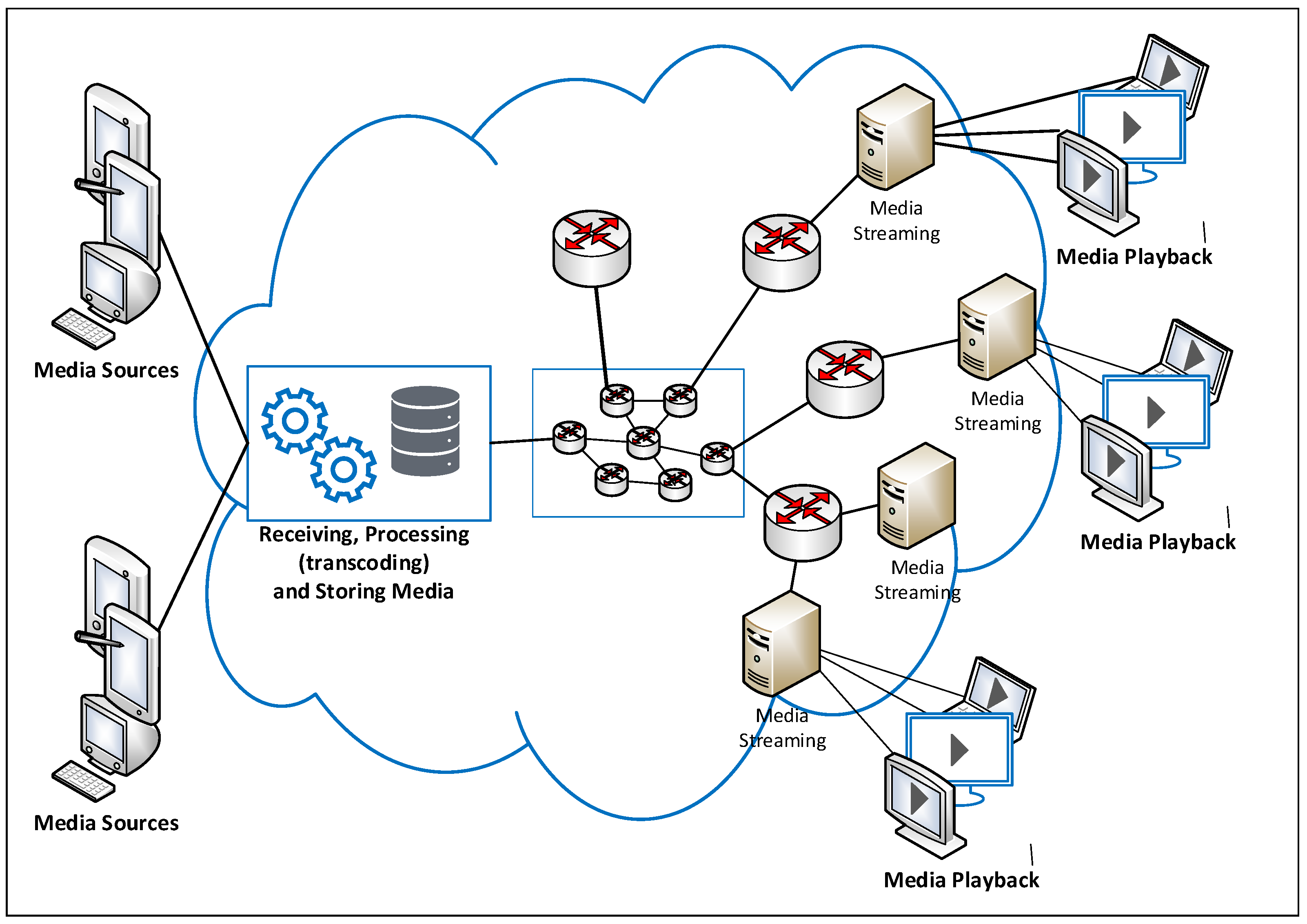
2.1. Considered Cloud-Based Streaming Architecture

In this paper, we consider the commonly used architecture for cloud-based on-demand and live streaming applications (such as Amazon CloudFront media streaming [24], IBM Video Streaming [25], Microsoft Azure Media Service [26] and Google Video Streaming services [27]). The architecture allows the user of the service to create a streaming application by enabling a chain (or pipe) of video processing starting from the video supply (live or recorded content) until video streaming to the potential clients of the enabled application. The nodes in the chain are often deployed as virtual machines or containers in the cloud.
As illustrated in Figure 1, the different services (video reception, processing, storing and streaming) are often running in virtual machines or containers.
A management tool is used to control and orchestrate the virtual machines (VMs)/containers involved in the application pipe/chain created in the cloud based on load balancing and VMs/containers health (processor load, memory load and network load) [24,25,26,27]. Streaming video nodes are often deployed on physical servers spread all over the world to be as close as possible to the final users. These nodes are connected to the main datacenter through private networks (most likely virtual private networks) often deployed on the Internet. Cloud companies have full control of routers, enabling private networks that allow multicast routing protocols to be activated over them to minimize the consumed bandwidth in the cloud backbone network. To avoid firewalls, HTTP-based streaming protocols are used where the video serves as small segments (chunks), such as web pages [5].
Generally, cloud-based streaming applications provide the client with a web page presenting the video catalog as HTML5 video tags, as done in YouTube, Dailymotion and Facebook video, for example. The links encoded on the page are generated to minimize the consumed resources in the cloud and offer the best possible user experience. The client is often redirected to the nearest video streaming node to him. As multicast routing is disabled on the Internet, each client is served through a unicast stream.
In this paper, we focus on minimizing the server node bandwidth as well as the consumed bandwidth in the network connecting the different nodes in the chain run by the cloud-based streaming application. This is portrayed as a set of interconnected network devices in the cloud/CDN of Figure 1.

2.2. Previous Work

Many research works have paid attention to the optimization of resource consumption in clouds. While some of them focused on the VM/container to physical node (server) placement (VMP) [28,29,30,31] problem, other works investigated the virtual network embedding (VNE) [32] problem. Solving the VMP problem aims to efficiently use the physical processing nodes (servers) while deploying virtual nodes (VMs/containers) on the cloud infrastructure. Some works considered [28,29,30,31] application needs in their optimization algorithms. However, other works targeted the trade-off between power consumption and cloud performance in fulfilling application needs [33,34,35,36]. The VNE problem solving [32,37,38,39,40,41] considers the link load between the nodes involved in the deployment of an application in the cloud (as well as Internet service providers (ISP) networks) in addition to the node load. The set of nodes and links builds a virtual network to be embedded on top of the physical datacenter’s infrastructure. The main goal here is to ensure a balanced use of the available physical resources, namely, the processing (servers) and network (switchers, routers and links) nodes. Network slicing [42,43] has been also considered in the cloud context to efficiently organize the bandwidth sharing among concurrent VMs hosted in the same physical node. While the works in this thematic (network slicing) deal with inter-slices optimization and efficient management, we rather consider in this work the intra-slice consumed bandwidth minimization.
In this paper, we suppose the existence of the virtual network in the cloud datacenter, and we aim to optimize the way the SNs (streaming nodes) share the video streams requested through the storage nodes. As mentioned in the Introduction, proactive and reactive video broadcasting protocols have been proposed to minimize the servers and network bandwidth.
Proactive protocols are subdivided into three subcategories. They are based on the same idea, which consists of dividing the video into many segments to be streamed through several channels. The size of each segment and the scheduling of the different segments among the various channels vary from one subcategory to another. The first subcategory is staggered broadcasting (SB) [6,18,44,45,46]. Given n channels and a movie of duration D, SB divides the movie into n equally sized segments. The n instances of the same movie are broadcast on n separate channels repeatedly, where each instance is shifted from the previous instance by the size of one segment, namely, D n . The second subcategory is called pyramid broadcasting. Protocols in this subcategory are based on the pyramid broadcasting protocol (PB) [6,16,20,22]. Having n channels, PB divides each movie into n segments with sizes growing geometrically with the parameter α > 1 . The first channel repeats broadcasting the first segment, the second channel repeats broadcasting the second segment, and so on for the remaining channels. The client must download data simultaneously from all channels to obtain a continuous fluid video display. Data must be downloaded at a rate equal to n times the playback (displaying) rate. A more efficient protocol named the Pagoda Broadcasting Protocol was proposed (PaB). PaB [6,47,48] uses a more complicated segment-to-channel scheduling algorithm. It distributes segments over the channels using the series {1,3,5,15,25}. Apart from the first channel where the first segment is broadcast repeatedly, PaB uses the remaining channels in a pairwise manner. The client also has to download data from all channels at once. PaB is better than all protocols of this subcategory in terms of the required server bandwidth while maintaining the same waiting time. A more efficient algorithm was proposed in [49]. Like PaB, it does not schedule segments to a channel in a sequential manner. It outperforms PaB because it is based on a more complicated heuristic to schedule segments to channels. In [50], the authors invented a new heuristic for segment-to-channel scheduling that enhances the performance of the version given in [49] in terms of the consumed bandwidth. The third subcategory is named the Harmonic Broadcasting (HB) HB [21,51]. It is based on the harmonic broadcasting protocol proved to be the best protocol [18] in terms of the required server bandwidth. HB divides each movie into equally sized segments, where each segment is broadcast through a separate channel. The channel bit rates are in decreasing order: the first channel bit rate is equal to the playback (displaying) rate denoted b, the second channel bit rate is equal to b 2 , the third is equal to b 3 , etc. The client must download data from all channels at the same time to obtain a smooth video display.
Some proactive protocols use a sequential segment to channel scheduling, namely, SB, PB and HB, while others such as PaB use a different segment to channel scheduling. We can then categorize proactive protocols based on these criteria. On the other hand, some proactive protocols oblige clients to wait for a fixed delay before starting the video display. These protocols are called fixed delay broadcasting protocols [52]. Fixed delay pagoda broadcasting (FDPB) is considered the most efficient fixed delay protocol [52] in terms of the consumed network and server bandwidth. The most well-known reactive protocol is stream tapping (ST) [15]. ST assumes that each customer set top box (STB) includes a buffer capable of storing several minutes of video. This buffer allows the client to tap into the current streams originally created for previous clients having requested the same video. The first client receives the requested movie on a special stream called the complete stream (CS). Further late clients requesting the same movie are served through temporary streams called full tap streams (FTS) to download the missed part of the movie. While displaying this first part of the movie using an FTS, video from a chosen ongoing complete stream is stored in the buffer. When the frame to be displayed from the FTS is the same as the first frame stored from the CS stream, the client terminates his FTS and begins displaying from its buffer, which continues to be fed from the corresponding CS. Unfortunately, this protocol performs worse than proactive protocols at a high workload [18] as the consumed bandwidth increases very rapidly with the number of clients demanding the same movie. A more recent reactive protocol is the Split and Merge Protocol, SAM [12]. Upon the arrival of the first client, SAM initiates a predefined batch time interval. All clients arriving within this batch interval will be served by the same video stream, called the S stream (equivalent to the CS in ST but no FTS is used in SAM), which is opened at the end of this time interval. In addition, SAM is an interactive protocol; it handles interactive operations through special streams called interactive streams (I stream) and the use of a client (synchronized) buffer. When a client performs an interactive operation, he will be served through a new I stream until he can be merged to an ongoing S stream through his synchronized buffer. In [8], the authors proposed the Dyadic optimal algorithm in terms of the consumed bandwidth when the request arrival time sequence is known (optimal for offline scenario) beforehand. The optimal solution is determined by dynamic programming. It has been shown by the authors in [8] that optimal stream sharing algorithms (including Dyadic) are very complex to implement. Hence, a trade-off between the performance and the complexity of implementation should be assured when designing the broadcasting protocol. While proactive protocols are recommended to broadcast frequently requested movies, reactive protocols should be used when the client arrival rate is low. In a recent work, the authors proposed reactive broadcasting protocols named slotted stream tapping (SST) [11,23]. This protocol performs like proactive protocols at a high workload and like reactive protocols at a low workload. It is based on the same ST Broadcasting scheme. The novelty of SST is to consider a slotted time axis where all clients arriving within one slot obtain their CS (or FTS) at the beginning of the next slot.
In Table 1, we summarize the principles and the performances (the consumed bandwidth) of the representative related works. Through, this table we can make the following observations:
  • In reactive protocols: Dyadic is outperforming Unicast, ST and SST techniques in terms of bandwidth consumption. But, it is very hard to implement as reported in [8]. This raises the following question: Could we assure a trade off between the bandwidth consumption and the implementation level of difficulty in the reactive category?
  • In proactive protocols: modern HTTP streaming protocols are based on (1) dividing the video into equally-sized segments and (2) sending them to the client as fast as segments are ready. SB is the only protocol compliant with these two properties (of modern streaming protocols). Unfortunately, its segments to channels scheduling is not optimal in terms of the consumed bandwidth. This raises the following question: How could this scheduling problem be stated and solved?
To answer the aforementioned two questions, we propose in this paper new streaming techniques, namely, SASST as a reactive technique for unpopular video streaming and NOPP as a proactive optimal technique for popular video streaming. Both proposed techniques minimize the server and the internal cloud (or CDN) streaming bandwidth. Since only one quality (the highest) is considered by SASST and NOPP, we suppose that any video adaptation (transcoding) mechanism is done by the streaming nodes on the fly.

3. Optimizing Cloud-Based Streaming Internal Bandwidth: Case of an Unpopular Video

For unpopular content streaming, in this section we present a new variant of the protocol Slotted Stream Tapping called SASST. We consider the on-demand scenario (not the live scenario) where video and/or audio files stored in the cloud storage nodes are requested.
First, we describe the SASST principle. Then, we evaluate the performances of SASST in terms of the average consumed bandwidth for both cases of (1) a deterministic high load and (2) a Poisson load of SN request arrivals.

3.1. SASST Principle

As SST is the baseline of the SASST technique, we begin by being reminded of the SST principle; then, we detail how SASST varies from SST. We choose SST as the baseline, as it was proven in [11,23] to be competitive in terms of performance and ease of implementation with regard to the other reactive protocols.

3.1.1. SST Principle

Each streaming node (SN) acts as a proxy node that loads the stream (back-end stream) from the storage node in the cloud and forks it to the clients requesting it. When the first streaming node requests the back-end stream, the storage node begins streaming it internally in the cloud network through a multicast complete stream (CS). When another streaming node later requests the same back-end stream, it will be asked (by the storage node using a manifest file, for example) to share the CS with the first streaming node and will be assigned a new multicast FTS stream to recover the missed video part (as it comes later than the first SN). The video content downloaded from the shared CS is buffered in a circular buffer, while the video content downloaded from the FTS is immediately relayed to the front-end clients. When the missed part is completely recovered, the FTS is closed, and the streaming continues through the circular buffer. This is the principle of the original version of SST. Recall that a slotted time axis is considered where all the requests coming within the same slot are served through the same CS and/or FTS starting from the beginning of the next slot.
Figure 2 portrays the SST principle. It contains four subfigures numbered from 1 to 4 illustrating how SST deals with late requests. As shown in subfigure 1, the first SN is served through a CS.
Then, as portrayed in subfigure 2, the second SN comes two slots later than the first SN. The second SN is assigned, as portrayed in subfigure 3, an FTS to serve the missed video slots 1 and 2 while buffering video slots 3 and 4 in a circular buffer from the ongoing CS. Finally, as missed slots 1 and 2 are recovered, the FTS is closed, and video streaming to clients continues through the circular buffer, as shown in subfigure 4 of Figure 2.
The circular buffer serves clients from one end while being filled through the CS from the other end. In other words, it serves slot 3 while being filled with slot 5, it serves slot 4 while being filled by slot 6, and so on, until the end of the requested video file. Thus, the buffer size of the second SN illustrated in Figure 2 never exceeds 2 slots, which is equal to the missed slot duration.

3.1.2. SASST Variant

The original version of SST does not consider FTS sharing between the latest streaming nodes. In this paper, we consider the sharing of FTS between them to further minimize the consumed bandwidth. Figure 3 represents the FTS handling with SST and SASST at a high workload where at least an SN request comes per slot. It can be seen that FTSs are shorter in the SASST case illustrated in Figure 3b than in the SST case shown by Figure 3a. Let’s take the example of the 8th SN node. As it arrives during the 7th time slot, using SST, it will be assigned a 7 slot FTS duration to serve the 7 missed slots. However, with SASST, it will only be assigned a 4 slot FTS duration (8th SN FTS), which saves 3 time slots compared to SST. This is because the 8th SN node obtains video slots 2, 4 and 6 through the 7th SN FTS and obtains video slots 1, 3, 5 and 7 through the 8th SN FTS. Hence, any late SASST SN node will share the FTS opened for the previous SN to further reduce the consumed bandwidth with regard to SST. Recall that SN requests that are received within the same time slots share the same FTSs.
SASST could be easily implemented over IP multicast using Real Time Protocol (RTP) or multicast-HTTP over QUIC. The SN needs to know the currently opened CS and FTS through a session description or announcing mechanism. Session Description Protocol (SDP) or DASH like manifest files could be used in this context. Once done, it starts downloading the video slots through multicast channels as described in the previous paragraph. The storage node could push the video slots using RTP or HTTP/3 packets.

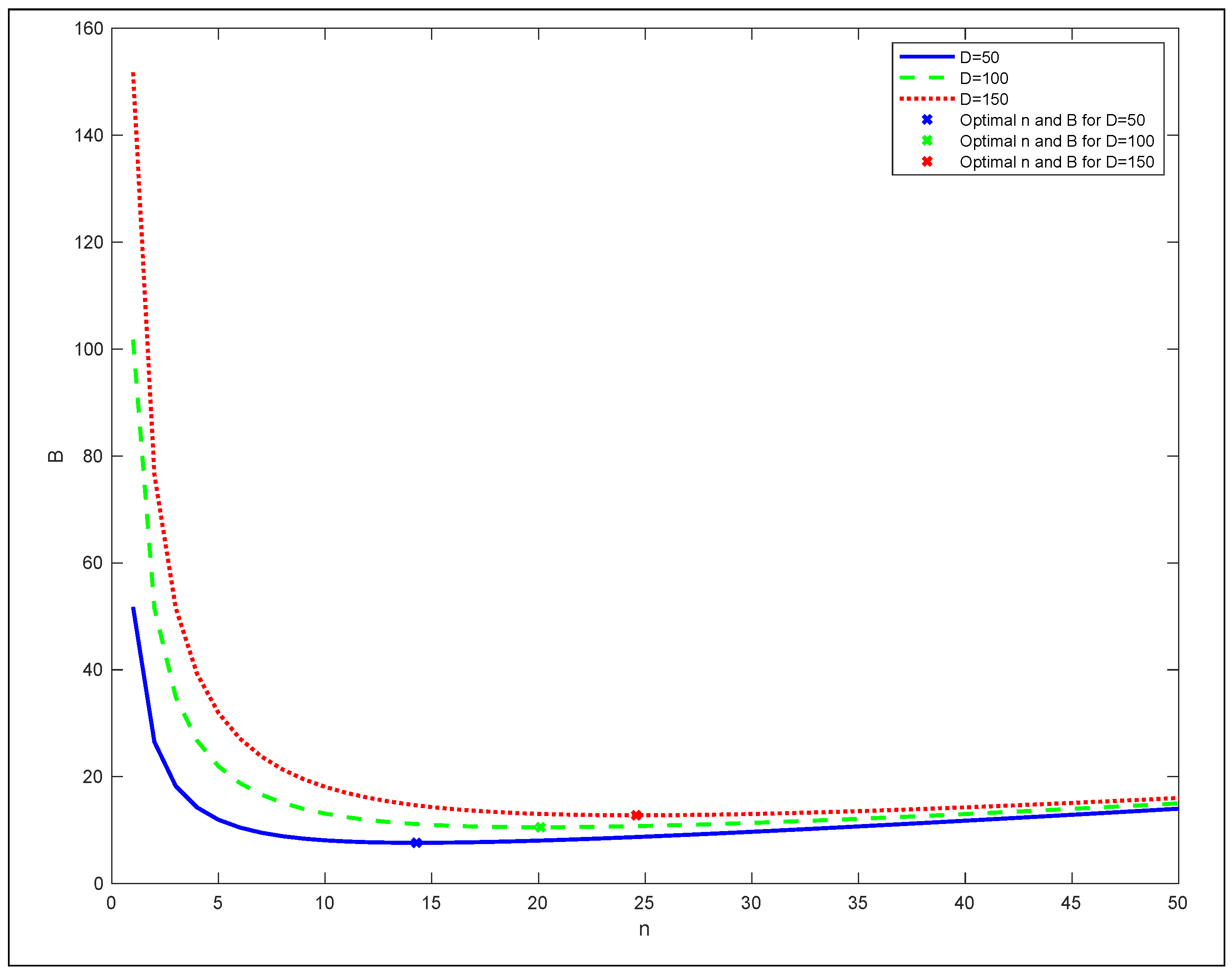
3.2. SASST Performance Evaluation: Case of a Deterministic High Load

As portrayed in Figure 3b, we consider in this subsection the deterministic high load scenario where we have at least one SN request per time slot.
Let l be the number of missed video slots by a late SN request, a s be the number of slots streamed through and FTS and b t be the number of slots tapped into (shared through) the FTS opened to the previous late SN request, as represented in boxes with orange color in Figure 3b.
We have
l = a s + b t
Let us recursively instantiate Equation (1) to each SN arrival of Figure 3b,
1 = 1 s + 0 t , 1 s : slot   1   which   is   streamed   through   the   2 nd   SN   FTS
2 = 2 s + 0 t , 2 s : slot   1   and   slot   2   are   streamed   through   the   3 nd   SN   FTS
3 = 2 s + 1 t , 2 s : slot   1   and   slot   3   are   streamed   through   the   4 nd   SN   FTS 1 t : slot   2   is   tapped   through   the   3 nd   SN   FTS
n = ( n 2 + 1 ) s + ( n 2 1 ) t   if   n   is   even o r
n = ( n + 1 2 ) s + ( n 1 2 ) t   if   n   is   odd
At a given value of l = n , the storage node should decide to open a CS instead of an FTS to a new SN request to minimize the consumed bandwidth and then start a new cycle. The average bandwidth value denoted B is the same in each cycle and is stated as follows:
B ( n ) = S C S ( n ) + S F T S ( n ) n
where S C S ( n ) denotes the number of video slots streamed through CSs and S F T S ( n ) denotes the number video slots streamed through FTSs during a cycle duration of n time slots.
At the stationary regime, the storage node opens a CS for each n slot. Thus,
S C S ( n ) = D n n = D
where D is the CS duration.
To determine S F T S , let us first consider the case of n being even. By summing the first terms a s of Equations (2)–(5), we obtain
S F T S ( n ) = 1 + 2 i = 2 n 2 i + ( n 2 + 1 ) = n 2 4 + n 2 + 1 .
When n is odd, we obtain by summing the terms a s of Equations (2)–(6) (except Equation (5)),
S F T S ( n ) = 1 + 2 i = 2 n + 1 2 i = n 2 4 + n 1 4 .
Replacing S C S ( n ) and S F T S ( n ) in Equation (7) by their expressions determined in Equations (8)–(10), respectively, gives
B ( n ) = D + 1 n + n 4 + 1 2 , if   n   is   even D 1 4 n + n 4 + 1 , if   n   is   odd .
Plotting B for three different values of video duration D = 50 , D = 100 and D = 150 shows that we can optimize B with regard to n, as portrayed in Figure 4.
The optimal value of n denoted as n * could be determined by resolving d B d n = 0 , which gives
n * = 2 D + 1 , if   n   is   even 2 D 1 4 , if   n   is   odd .
Thus, we can determine the optimal average bandwidth value denoted as B * by replacing n * in Equation (11),
B * ( n ) = D + 1 + 1 2 , if   n *   is   even D 1 4 + 1 , if   n *   is   odd .

3.3. SASST Performance Evaluation: Case of a Probabilistic Load

In this case, we suppose that the SN request interarrival follows a random variable. Let us denote the average time slots separating two successive requests by y. By applying a recursive Equation (1) to each SN arrival, we obtain
y = y s + 0 t
2 y = 2 y s + 0 t
3 y = 2 y s + 1 y t
n y = ( n 2 + 1 ) y s + ( n 2 1 ) y t   if   n   is   even o r
n y = ( n + 1 2 ) y s + ( n 1 2 ) y t   if   n   is   odd .
By following the same steps as in Section 3.2 (i.e., summing the a s of Equations (14)–(17) if n is even and to (18) if n is odd), we can determine the total FTS slot number denoted as S y F T S for n being even and odd as follows:
S y F T S ( n ) = y [ 1 + 2 i = 2 n 2 i + ( n 2 + 1 ) ] = y [ n 2 4 + n 2 + 1 ] , if   n   is   even y [ 1 + 2 i = 2 n + 1 2 i ] = y [ n 2 4 + n 1 4 ] , if   n   is   odd .
Hence, we can deduce the expression of the average bandwidth value, denoted as B y , consumed by a storage node as follows:
B y ( n ) = D y + 1 n + n 4 + 1 2 , if   n   is   even D y 1 4 n + n 4 + 1 , if   n   is   odd .
After Resolving d B y d n = 0 , we obtain,
n * = 2 D y + 1 , if   n   is   even 2 D y 1 4 , if   n   is   odd .
Let us replace n * in B y ; then we obtain the optimal value of B y denoted B y * ,
B y * ( n * ) = D y + 1 + 1 2 , if   n *   is   even D y 1 4 + 1 , if   n *   is   odd .
Assume that the SN request interarrival is an exponential random variable. We can conclude the probability p 0 of having zero arrival per time slot s as follows:
p 0 = e λ s
where λ is the Poisson average arrival rate.
Let Y be a random variable denoting the number of slots k between two Poisson successive requests, defined by
P [ Y = k ] = p 0 k 1 ( 1 p 0 )
As y is the average interarrival slot number between two successive requests, we can then express it as follows using Equations (23) and (24):
y = k = 1 + k P [ Y = k ] = 1 1 e λ s .
Replacing y by its expression in Equation (22) gives the following:
B y * ( λ ) = D 1 1 e λ s + 1 + 1 2 , if   n *   is   even D 1 1 e λ s 1 4 + 1 , if   n *   is   odd .
As lim λ y = 1 , we can deduce the asymptotic values of n * and B * as follows:
lim λ n * ( λ ) = 2 D + 1 , if   n   is   even 2 D 1 4 , if   n   is   odd .
lim λ B * ( λ ) = D + 1 + 1 2 , if   n *   is   even D 1 4 + 1 , if   n *   is   odd .
This shows that the deterministic high load performances done in Section 3.2 are upper bounds of the probabilistic performances of SASST. Another important result achieved through Equation (28) is that the average bandwidth of SASST is less than the average bandwidth of SST, which was expressed in [11,23] as B S S T * = 2 D 1 2 for long videos where D > 3.5 when n * is even and for D > 4.5 when n * is odd. Recall that SST was proven to outperform ST in terms of the average consumed bandwidth in [11,23].

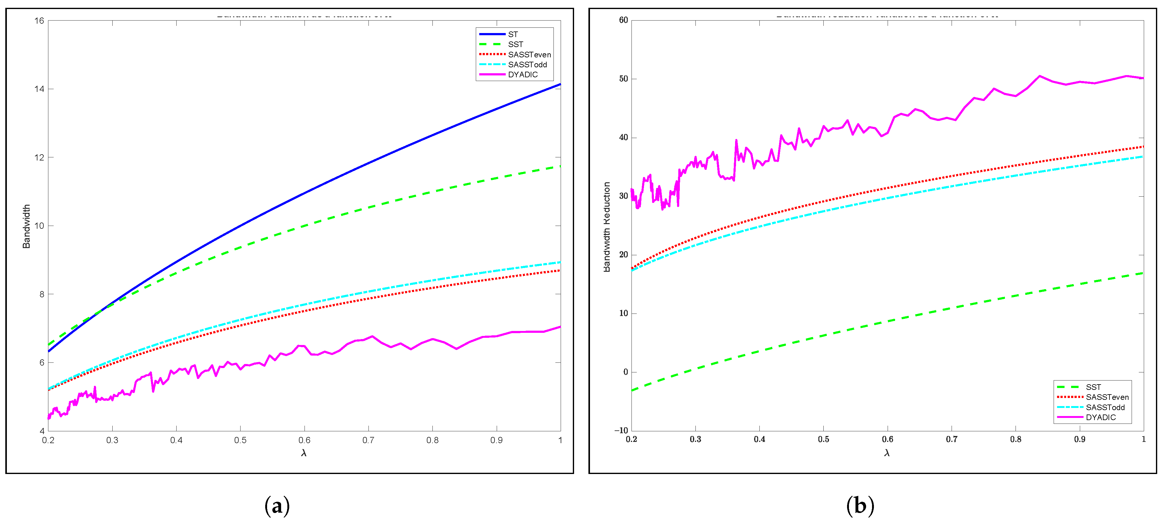
3.4. SASST Performance Evaluation: Numerical Analysis

In this subsection, we compare SASST to SST, ST and Dyadic in terms of the average consumed bandwidth as a function of the SN request rate denoted as λ . As we can see in Figure 5a, SASST outperforms SST and ST in terms of the average bandwidth except for request rates smaller than 0.06, where the performances are very close to one other. Note here that the video size D = 100 and one slot s = 1 .
However, Dyadic requires a lower bandwidth than SASST. The maximum difference between them reaches 1.65 streams for an arrival rate equal to 1. In fact, having one or many requests per slot does not affect the performance in terms of the consumed bandwidth. Thus, SASST is very competitive in terms of the consumed bandwidth while being simpler than Dyadic with regard to the complexity of implementation.
The bandwidth reduction of SASST, SST and Dyadic compared to ST is plotted in Figure 5b. As we can see in this figure, SASST ranks second after Dyadic. At a high request rate ( λ 1 ), the bandwidth reduction values are almost equal to 50%, 39% and 18% for Dyadic, SASST and SST, respectively. Note that ST bandwidth is taken as reference.
To obtain more insight into the optimal value of ( n * ) with regard to the video size D using SASST, in Figure 6 we plot n * D for odd and even cases of n * where D { 10 , 11 , 1000 } . As can be seen, as the video size increases, the storage node decides to open CS more frequently than if the video size is smaller. This could be explained by the rapid growth of cumulative FTS sizes that quickly reach the size of the video, which encourages opening a new CS rather than an FTS for the current late SN request. Indeed, serving late requests with a smaller FTS if a new CS is opened is better than serving the late requests with very long FTSs in terms of bandwidth minimization.

4. Optimizing Cloud-Based Streaming Internal Bandwidth: Case of Popular Video

In this section, we study the case of a high SN request rate where it is recommended to use a proactive streaming protocol. Unlike the reactive protocols (such as SASST presented in the previous section), the storage node divides the video into equally-sized segments and broadcasts the them repeatedly on a set of multicast channels regardless of the SN requests using a schedule that allows the SN to obtain all video segments. We aim to determine the optimal segments-to-channels scheduling in terms of consumed bandwidth. This scheduler will be used in the context of NOPP.
In the rest of the current section, we analyze how SASST could be approximated by the proactive protocol staggered broadcasting. Although it is out of the scope of this paper, this approximation helps in implementing a smooth transition from using reactive protocol a proactive one when the video becomes popular at runtime. Then, we detail the formulation and solving process of the bandwidth optimization problem which leads to NOPP optimal scheduling of segments to broadcasting channels. Two version are considered: (1) minimizing the bandwidth when the streaming period of a given video is known in advance (known time horizon) and (2) when it is not (periodic).

4.1. Approximating SASST by SB

When the system is in a stationary regime, the storage node opens a new CS each n * slots of time. Thus, we can see the CS streaming channels as portrayed in Figure 7a. If we consider each n * in a given CS as a video segment and we name it s e g m e n t i where i { 1 , 2 , 3 , , N } (we assume here that D n * = N ), then we obtain the same broadcasting schema as SB [6,18]. Each channel broadcasts one instance of the video shifted by the size of one segment from the previous and the next adjacent channels. This means that one instance of the entire video is broadcast across all channels in each segment duration period. Hence, any SN can download the entire video if it connects to all the channels at the same time after one time slot. Using SB, any SN could download the entire video by connecting to only one channel during the CS duration to download the video segments one by one.
The question is how to minimize the number of broadcasting channels while allowing the SN to download the video without missing any segment. The key scheduling answer to this question is to broadcast each segment i at least once on any of the channels each i time slots. By time slot, we mean one segment duration (i.e., equal to n * slots). This property is inherited from the playback continuity property, where a video player must find segments i available for playback immediately after playing the i 1 previous segments. In other words, segment i should be downloaded during the playback period of the previous segments or should be immediately available on one of the channels for playback. Figure 7b shows an optimal scheduling of the 17 segments initially broadcast by SASST. As portrayed in Figure 7a, the streaming bandwidth drops from 17 to 4 broadcasting channels for the same video.
This scheduling problem has been proven to be NP-hard in [50]. Nevertheless, for a fixed video broadcasting time horizon, we can afford to solve the scheduling problem through an exact method using a linear program formulation. Through a fixed time horizon, we mean that we know for how long we will keep streaming (broadcasting) the video. The optimization problem formulation is presented in the next subsection. For the case of an unknown time horizon, we propose in Section 4.3 a different formulation of the problem to preserve a reasonable solving cost with regard to the formulation of the fixed time horizon described in Section 4.2. NOPP is based on the two proposed versions of optimal schedules (known and unknown time horizons).

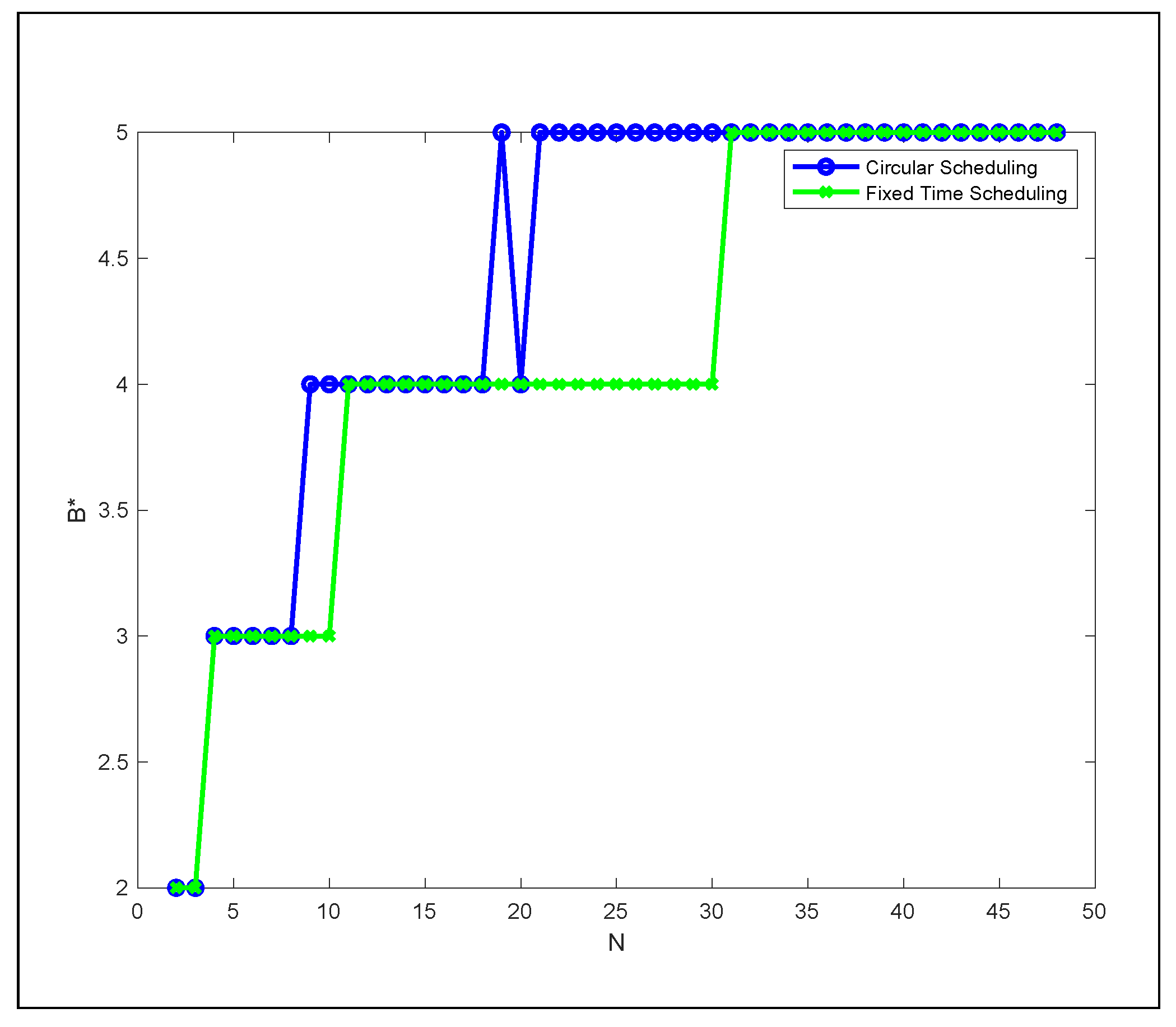
4.2. Linear Program Formulation for a Fixed Time Horizon

Let C be the fixed broadcasting time horizon and N be the total number of equally sized segments of the media. Generally, C is equal to n * N with ( n > 1 ). Let x i j be a Boolean variable indicating whether or not segment i can be scheduled within time slot j ( x i j = 1 ) ( x i j = 0 ) and B be the total number of broadcasting network channels, which is the total consumed bandwidth (expressed in number of channels) used by NOPP.
Our Linear Program (LP) can be stated as follows:
Minimize   B
Subject   to :
j = 1 N x j t B , t { 1 , 2 , , C } k = t t + j 1 x j k 1 , j { 1 , 2 , , N }
and   t { 1 , 2 , , C j + 1 }
i = 1 N 1 i B N x j , t { 0 , 1 } , j { 1 , 2 , , N }
and   t { 1 , 2 , , C }
B N *
Constraint (30) means that the number of scheduled segments for any time slot cannot exceed the total number of channels. Constraint (31) means that each segment i must be scheduled at least once for any time window of size i slots. The lower bound used in constraint (32) has been determined in [18,50].
Solving the LP using the Gurobi solver [53] for N = C , N { 2 , 3 , , 50 } gives the results summarized in Table 2. Note that the solver was installed on a 16 processors Linux workstation with 2.4 GHz speed each.
The main drawback with fixed time horizon scheduling is the obligation to stop serving SN requests before a period of time equal to the size of a video instance (only the SN arriving within C-N are served). Indeed, the requests coming during the streaming time of the last instance of the video will not be able to download the entire segments. As shown in Figure 8, a request coming during the third time slot will miss segment 10. An additional time slot is therefore needed to schedule it (segment 10). We need to add an increasing number of time slots to schedule as many missed segments as we have new requests during this last instance of the media.
Unfortunately, this is not obvious, as the repetition of the same optimal schedule does not guarantee a feasible schedule.
As we can see in Figure 9, the distance between two successive occurrences of each of the segments 6, 7, 8 and 9 is equal to 10 (one occurrence is counted in the distance), which violates the playback property where segment i must be scheduled at least once in any i successive slots. As portrayed in the figure, only 3 segments among 4 could be scheduled in the free places (in green), which means that the obtained scheduling is not feasible.
To overcome this problem, we propose in the next subsection a new LP model that allows us to obtain an optimal schedule that could be repeated as many times as we have new requests without violating the playback propriety.

4.3. Linear Program Formulation for an Unknown Time Horizon

The main change in the new LP model with regard to the fixed time horizon model is the periodicity constraint. This guarantees the playback property when repeating the optimal schedule. The LP formulation is stated as follows:
Minimize   B
Subject   to :
j = 1 N x j t B , t { 1 , 2 , , C } k = t t + j 1 x j k 1 ,
j { 1 , 2 , , N } if   t C j + 1 k = t C x j k + k = 1 j ( C t + 1 ) x j k 1 ,
if   C j + 1 t C
i = 1 N 1 i B N x j , t { 0 , 1 } , j { 1 , 2 , , N }
and   t { 1 , 2 , , C }
B N *
All the constraints are the same as the previous LP, except constraints (37) and (39), where we consider circular scheduling. They guarantee that a segment i is scheduled at least once in any successive i slots from slot j to slot C and from slot 1 to slot i ( C j + 1 ) . Note here that the minimum time horizon C for a circular schedule is equal to the video size N.
Solving the periodic LP for N = C = 10 using a Gurobi solver [53] gives the optimal circular schedule portrayed by Figure 10.
Table 3 summarizes the solving results of the periodic LP for N { 2 , 3 , , 48 } .
Using the circular optimal schedule, the storage node allocates one more time slot to stream the segments indicated by the optimal schedule on the broadcasting channels for any newly arriving SN request where the distance between the newly allocated slot and the arrival slot is equal to N. As shown in Figure 10, a request arriving at slot 1 induces allocating slot 11 to broadcast segments 1, 2, 6 and 10.
The plots in Figure 11 show that fixed time schedules could be naturally periodic (circular). The optimal bandwidth value B * is the same for many configurations considered in fixed time and circular schedules. This proves that at least one optimal schedule exists for a fixed time horizon version that is naturally periodic.
Through Figure 11 plots, we can observe that in the time horizon value C = 20 , the optimal bandwidth value B * decreases by 1. Thus, we can ask the following open question: what are the time horizon values of C that minimize the bandwidth B for a given video size N?

4.4. NOPP Deployment

To deploy NOPP, the following tasks should be performed::
  • The administrator of the streaming system should set (1) the number of segments of the video and (2) the streaming time horizon. in the system ggraphical interface If he wants to use a periodic scheduling, then he should indicate that instead of the time horizon.
  • The system solves either the first version (with fixed time horizon) or the second version (periodic) of the LP. A manifest file containing the optimal scheduling is then generated and stored in the storage node with video segments.
  • The SN starts by requesting the manifest (of the session description) file from the storage node to know how to reorder the arriving segments. Then, it starts the download of video segments, the reordering and the streaming to the Internet users’ devices. The storage node could use RTP or HTTP/3 to push the video segments.

5. Conclusions

In this paper we proposed cloud streaming bandwidth optimization techniques. For unpopular video cases, we presented a new variant of the Slotted Stream Tapping (SST) protocol called Share All SST (SASST). We analytically proved that SASST reduces the storage node bandwidth by almost 30% and 20% compared to stream tapping (ST) and SST, respectively. However, Dyadic further reduces the bandwidth by almost 10% compared to SASST while being harder to implement, as shown in [8]. We discussed how SASST could be smoothly turned on a proactive protocol to also serve popular videos. To minimize the bandwidth, we proposed two LP formulations to obtain the optimal segments to channel schedules for known and unknown time horizons. We showed how the optimal schedule for the unknown time horizon case could be repeated infinitely to serve new incoming requests. We called the new broadcasting protocol based on these optimal schedules the New Optimal Proactive Protocol (NOPP). As it is optimal, it outperforms the rest of the proactive broadcasting techniques of the literature in terms of the consumed server and network bandwidth. In the future, we plan to bring the proposed techniques into practice, which requires studying in depth the possible ways to change segment-based streaming protocols, such as HLS, to minimize the steaming bandwidth in a multicast enabled network.

Author Contributions

Conceptualization, A.G. and L.H.; methodology, A.G.; software, A.G.; validation, A.G., B.B.Y. and M.K.; formal analysis, A.G., L.H. and M.K.; writing—original draft preparation, A.G.; writing—review and editing, A.G., M.K. and B.B.Y. All authors have read and agreed to the published version of the manuscript.

Funding

This research was funded by the Deanship of Scientific Research at King Saud University through research group no. RG-1439-001.

Institutional Review Board Statement

Not applicable.

Informed Consent Statement

Not applicable.

Data Availability Statement

Not applicable.

Acknowledgments

The authors extend their appreciation to the Deanship of Scientific Research at King Saud University for funding this work through research group no. RG-1439-001.

Conflicts of Interest

The authors declare no conflict of interest.

References

  1. Cisico: Cisco Annual Internet Report (2018–2023) White Paper. 2018. Available online: https://www.cisco.com/c/en/us/solutions/collateral/executive-perspectives/annual-internet-report/white-paper-c11-741490.html (accessed on 1 July 2021).
  2. Adobe. 2015. Available online: http://www.adobe.com/products/hds-dynamic-streaming.html (accessed on 6 January 2021).
  3. Apple: HTTP Live Streaming. 2015. Available online: http://tools.ietf.org/html/draft-pantos-http-live-streaming-12 (accessed on 6 January 2021).
  4. Microsoft. 2015. Available online: http://www.iis.net/downloads/microsoft/smooth-streaming (accessed on 6 January 2020).
  5. Stockhammer, T. Dynamic adaptive streaming over http–: Standards and design principles. In Proceedings of the Second Annual ACM Conference on Multimedia Systems, San Jose, CA, USA, 23–25 February 2011; pp. 133–144. [Google Scholar]
  6. Carter, S.W.; Long, D.D.E.; Pâris, J.F. Video-on-Demand Broadcasting Protocols. 2000. Available online: citeseer.ist.psu.edu/carter00videodemand.html (accessed on 6 January 2020).
  7. Pardue, L.; Bradbury, R.; Hurst, S. Hypertext Transfer Protocol (HTTP) over Multicast QUIC Internet Engineering Task Force. Draft-Pardue-Quic-http-Mcast-09. August 2021. Available online: https://www.ietf.org/id/draft-pardue-quic-http-mcast-09.html (accessed on 20 November 2021).
  8. Bar-Noy, A.; Goshi, J.; Ladner, R.E.; Tam, K. Comparison of stream merging algorithms for media-on-demand. Multimed. Syst. 2004, 9, 115–129. [Google Scholar] [CrossRef]
  9. Carter, S.R.; Paris, J.F.; Mohan, S.; Long, D.D.E. A dynamic heuristic broadcasting protocol for video-on-demand. In Proceedings of the IEEE 21st International Conference on Distributed Computing Systems (ICDCS ’01), Washington, DC, USA, 7–10 July 2001; p. 657. [Google Scholar]
  10. Eager, D.; Vernon, M.; Zahorjan, J. Optimal and Efficient Merging Schedules for Video-on-Demand Servers. In Proceedings of the Seventh ACM International Conference on Multimedia (Part 1), Orlando, FL, USA, 30 October–5 November 1999; Available online: http://www.cs.usask.ca/faculty/eager (accessed on 20 January 2021).
  11. Gazdar, A.; Belghith, A. Slotted stream tapping. In Proceedings of the 2004 ACM Workshop on Next-Generation Residential Broadband Challenges (NRBC ’04), New York, NY, USA, 15 October 2004; ACM Press: New York, NY, USA, 2004; pp. 50–56. [Google Scholar] [CrossRef]
  12. Liao, W.; Li, V.O.K. The split and merge protocol for interactive video-on-demand. IEEE MultiMedia 1997, 4, 51–62. [Google Scholar] [CrossRef] [Green Version]
  13. Pâris, J.F.; Carter, S.W.; Long, D.D.E. A universal distribution protocol for video-on-demand. In Proceedings of the IEEE International Conference on Multimedia and Expo 2000, New York, NY, USA, 30 July–2 August 2000. [Google Scholar]
  14. Pâris, J.F.; Long, D.D.E. An analytic study of stream tapping protocols. In Proceedings of the IEEE International Conference on Multimedia and Expo (ICME 2006), Toronto, ON, Canada, 9–12 July 2006; pp. 1237–1240. [Google Scholar]
  15. Carter, S.W.; Long, D.D.E. Improving video-on-demand server effeciency through stream tapping. In Proceedings of the 6th International Conference on Computer Communications and Netrworks (ICCCN’97), Las Vegas, NV, USA, 22–25 September 1997; pp. 200–207. [Google Scholar]
  16. Aggarwal, C.C.; Wolf, J.L.; Yu, P.S. A permutation-based pyramid broadcasting scheme for video-on-demand systems. In Proceedings of the IEEE International Conference on Multimedia and Computing Systems, Hiroshima, Japan, 17–23 July 1996; pp. 118–126. [Google Scholar]
  17. Belghith, A.; Gazdar, A. Generalization of fixed delay broadcasting protocols. In Proceedings of the Third International Conference on Intelligent Computing and Information Systems, Cairo, Egypt, 15–18 March 2007. [Google Scholar]
  18. Hu, A. Video-on-Demand broadcasting protocols: A comprehensive study. In Proceedings of the Twentieth Annual Joint Conference of the IEEE Computer and Communications Society (Infocom’01), Anchorage, AK, USA, 22–26 April 2001. [Google Scholar]
  19. Hua, K.A.; Sheu, S. Skyscraper broadcasting: A new broadcasting scheme for metropolitan video-on-demand systems. ACM SIGCOMM Comput. Commun. Rev. 1997, 27, 89–100. [Google Scholar] [CrossRef]
  20. Juhn, L.S.; Tseng, L.M. Fast broadcasting for hot video access. In Proceedings of the Internantional Workshop on Real-Time Computing Systems and Application, Taipel, Taiwan, 27–29 October 1997; pp. 237–243. [Google Scholar]
  21. Juhn, L.S.; Tseng, L.M. Harmonic broadcasting for video-on-demand service. IEEE Trans. Broadcast. 1997, 43, 268–271. [Google Scholar] [CrossRef] [Green Version]
  22. Viswanathan, S.; Imielinski, T. Pyramid broadcasting for video-on-demand service. Int. Soc. Opt. Eng. SPIE 1995, 24, 66–77. [Google Scholar]
  23. Gazdar, A.; Belghith, A. Hybrid broadcasting protocols: A comparative study. In Proceedings of the 2004 IEEE Symposium on Signal Processing and Information Technology (ISSPIT ’04), Rome, Italy, 18–21 December 2004. [Google Scholar]
  24. Amazon. Amazon Cloudfront Media Streaming Tutorials. Available online: https://aws.amazon.com/cloudfront/streaming/ (accessed on 5 July 2021).
  25. IBM. IBM Video Streaming Developers. Available online: https://developers.video.ibm.com (accessed on 10 January 2021).
  26. Microsoft. Azure Documentation. Available online: https://docs.microsoft.com/en-us/azure/?product=media (accessed on 10 January 2021).
  27. Google. Video AI. Available online: https://cloud.google.com/video-intelligence (accessed on 10 January 2021).
  28. Cao, G. Topology-aware multi-objective virtual machine dynamic consolidation for cloud datacenter. Sustain. Comput. Inform. Syst. 2019, 21, 179–188. [Google Scholar] [CrossRef]
  29. Farzai, S.; Shirvani, M.H.; Rabbani, M. Multi-objective communication-aware optimization for virtual machine placement in cloud datacenters. Sustain. Comput. Inform. Syst. 2020, 28, 100374. [Google Scholar] [CrossRef]
  30. Gopu, A.; Venkataraman, N. Optimal vm placement in distributed cloudenvironment using moea/d. Soft Comput. 2019, 23, 11277–11296. [Google Scholar] [CrossRef]
  31. Tian, H.; Wu, J.; Shen, H. Efficient algorithms for vm placement in cloud data centers. In Proceedings of the 2017 18th International Conference on Parallel and Distributed Computing, Applications and Technologies (PDCAT), Taipei, Taiwan, 18–20 December 2017; pp. 75–80. [Google Scholar] [CrossRef]
  32. Zhao, C.; Parhami, B. Virtual network embedding on massive substrate networks. Trans. Emerg. Telecommun. Technol. 2020, 31, e3849. [Google Scholar] [CrossRef] [Green Version]
  33. Rizvandi, N.B.; Taheri, J.; Zomaya, A.Y. Some observations on optimal requency selection in dvfs-based energy consumption minimization. J. Parallel Distrib. Comput. 2011, 71, 1154–1164. [Google Scholar] [CrossRef] [Green Version]
  34. Safari, M.; Khorsand, R. Energy-aware scheduling algorithm for time-constrained workflow tasks in dvfs-enabled cloud environment. Simul. Model. Pract. Theory 2018, 87, 311–326. [Google Scholar] [CrossRef]
  35. Stavrinides, G.L.; Karatza, H.D. An energy-efficient, qos-aware and cost-effective scheduling approach for real-time workflow applications in cloud computing systems utilizing dvfs and approximate computations. Future Gener. Comput. Syst. 2019, 96, 216–226. [Google Scholar] [CrossRef]
  36. Wu, T.; Gu, H.; Zhou, J.; Wei, T.; Liu, X.; Chen, M. Soft error-aware energy-efficient task scheduling for workflow applications in dvfs-enabled cloud. J. Syst. Archit. 2018, 84, 12–27. [Google Scholar] [CrossRef]
  37. Caggiani Luizelli, M.; Richter Bays, L.; Salete Buriol, L.; Pilla Barcellos, M.; Paschoal Gaspary, L. How physical network topologies affect virtual network embedding quality: A characterization study based on isp and datacenter networks. J. Netw. Comput. Appl. 2016, 70, 1–16. [Google Scholar] [CrossRef]
  38. Cheng, X.; Su, S.; Zhang, Z.; Wang, H.; Yang, F.; Luo, Y.; Wang, J. Virtual network embedding through topology-aware node ranking. SIGCOMM Comput. Commun. Rev. 2011, 41, 38–47. [Google Scholar] [CrossRef]
  39. Chowdhury, M.; Rahman, M.R.; Boutaba, R. Vineyard: Virtual network embedding algorithms with coordinated node and link mapping. IEEE/ACM Trans. Netw. 2012, 20, 206–219. [Google Scholar] [CrossRef]
  40. Fischer, A.; Botero, J.F.; Beck, M.T.; de Meer, H.; Hesselbach, X. Virtual network embedding: A survey. IEEE Commun. Surv. Tutor. 2013, 15, 1888–1906. [Google Scholar] [CrossRef]
  41. Li, J.; Zhang, N.; Ye, Q.; Shi, W.; Zhuang, W.; Shen, X. Joint resource allocation and online virtual network embedding for 5g networks. In Proceedings of the GLOBECOM 2017—2017 IEEE Global Communications Conference, Singapore, 4–8 December 2017; pp. 1–6. [Google Scholar] [CrossRef]
  42. Afolabi, I.; Taleb, T.; Samdanis, K.; Ksentini, A.; Flinck, A. Network Slicing and Softwarization: A Survey on Principles, Enabling Technologies, and Solutions. IEEE Commun. Surv. Tutor. 2018, 20, 2429–2453. [Google Scholar] [CrossRef]
  43. Aldulaimy, A.; Itani, W.; Taheri, J.; Shamseddine, M. bwSlicer: A bandwidth slicing framework for cloud data centers. Future Gener. Comput. Syst. 2020, 112, 767–784. [Google Scholar] [CrossRef]
  44. Gazdar, A.; Belghith, A. Etude et implémentation d’une solution interactive pour la diffusion de la vidéo dans les systèmes de vidéo à la demande. In Proceedings of the 2003 Sciences of Electronic, Technologies of Information and Telecommunications (SETIT ’03), Sousse, Tunisia, 17–21 March 2003. [Google Scholar]
  45. Gazdar, A.; Belghith, A. Discrete interactive staggered broadcasting. In Proceedings of the 2004 IEEE Consumer Communications and Networking Conference (CCNC ’04), Las Vegas, NV, USA, 5–8 January 2004. [Google Scholar]
  46. Gazdar, A.; Belghith, A. Une solution vod interactive continue. In Proceedings of the 2004 Colloque Africain sur la Recherche en Informatique (CARI ’04), Hammamet, Tunisia, 27–29 November 2004. [Google Scholar]
  47. Pâris, J.F.; Carter, S.W.; Long, D.D.E. Efficient broadcasting protocols for video-on-demand. In Proceedings of the the International Symposium on Modelling, Analysis, and Simulation of Computing and Telecom Systems, Montreal, QC, Canada, 19–24 July 1998; pp. 127–132. [Google Scholar]
  48. Pâris, J.F.; Carter, S.W.; Long, D.D.E. Combining pay-per-view and video-on-demand services. In Proceedings of the Modeling, Analysis and Simulation of Computer and Telecommunication Systems, College Park, MD, USA, 24–28 October 1999. [Google Scholar]
  49. Bar-Noy, A.; Ladner, R.E. Windows scheduling problems for broadcast systems. In Proceedings of the 13th ACM-SIAM Symposium on Discrete Algorithms (SODA), San Francisco, CA, USA, 6–8 January 2002. [Google Scholar]
  50. Bar-Noy, A.; Ladner, R.E.; Tamir, T. Scheduling techniques for media-on-demand. Algorithmica 2008, 52, 413–439. [Google Scholar] [CrossRef] [Green Version]
  51. Pâris, J.F.; Carter, S.W.; Long, D.D.E. A low bandwidth broadcasting protocol for video-on-demand. In Proceedings of the the 7th International Conference on Computer Communication and Networks, Lafayette, LA, USA, 12–15 October 1998; pp. 609–616. [Google Scholar]
  52. Yan, E.M.; Kameda, T. An efficient vod broadcasting scheme with user bandwidth limit. In Proceedings of the SPIE/ACM MMCN 2003, Santa Carla, CA, USA, 23 February 2003. [Google Scholar]
  53. Gurobi Optimization, LLC. Gurobi Optimizer Reference Manual. 2021. Available online: https://www.gurobi.com (accessed on 5 July 2021).
Figure 1. Cloud-Based Video Streaming Architecture.
Applsci 11 11267 g001
Figure 2. Illustration of the SST principle and how it handles late requests. In (1) the first SN request arrives and gets a CS. In (2) the second SN request arrives late for two slots. In (3) the Streaming node opens a FTS for the second SN to get the two missed slots while sharing the CS with first SN. In (4) the FTS is closed and the second SN continues getting the video from its buffer.
Applsci 11 11267 g002
Figure 3. Example of FTS handling with SST and SASST at a high workload. (a) SST FTS; (b) SASST FTS.
Applsci 11 11267 g003
Figure 4. SASST average bandwidth variation as a function of n.
Applsci 11 11267 g004
Figure 5. Comparison of bandwidth and bandwidth reduction between SASST, SST, ST and Dyadic as a function of the request arrival rate λ , respectively. (a) Bandwidth; (b) Bandwidth Reduction.
Applsci 11 11267 g005
Figure 6. Percentage of n * as a function of the total video size D for n * even and odd, respectively. (a) n * even; (b) n * odd.
Applsci 11 11267 g006
Figure 7. From proactive SASST to optimal scheduling of 17 segments. (a) SASST as SB; (b) Optimal Scheduling with 17 segments.
Applsci 11 11267 g007
Figure 8. An example of an optimal scheduling for N = C = 10 and B * = 3 . The request arrival slot is illustrated in black. The green video segments are successfully downloaded. The red video segment is missed.
Applsci 11 11267 g008
Figure 9. An optimal scheduling for N = C = 10 repeated twice. The distance between the two successive occurrences in red of video segment 6 is equal to 11. The distance between the two successive occurrences in orange of video segment 7 is equal to 11. The distance between the two successive occurrences in cyan of video segment 8 is equal to 10. The distance between the two successive occurrences in magenta of video segment 9 is equal to 10. They are all violating the playback property. Some free slots that could be assigned to some video segments are colored in green.
Applsci 11 11267 g009
Figure 10. An example of optimal circular scheduling for N = C = 10 . B * = 4 .
Applsci 11 11267 g010
Figure 11. B * as a function of N for circular and fixed time scheduling.
Applsci 11 11267 g011
Table 1. Summary of representative works, their principles and performances.
PrincipleBandwidthImplementation
Reactive
UnicastOpens a stream
for each client request.
B = λ D
λ is the request
rate,
D is the video
duration.
Easy.
ST [15]Makes clients sharing
one main stream (TS)
and provides the missed
part by an additional
unicast stream (FTS).
B = λ D + 1 1 Medium.
SST [11,23]In addition to what ST
does, SST groups
client request per slots
to be served through
the same streams.
B = 2 D 1 2 Medium.
Dyadic [8]Allows clients to share
all opened streams in a
pseudo-optimal way.
The arrival sequence
should be known in
advance to be optimal.
No analytical
expression.
Hard.
Proactive
SB [6,18,44,45,46]   Divides the movie into n
equally-sized segment
and broadcasts each
segment repeatedly in
a channel.
B = n Easy.
Pyramid
[6,16,20,22]
Divides the movie into
n segments with size
growing geometrically.
Each segment is
broadcast repeatedly
in a channel.
B = n ( D w n 1 ) ,
D is the video
duration,
w is the client
waiting time.
Hard.
Harmonic
[21,51]
Divides the movie into n
equally-sized segment
S 1 , S 2 , … S n and broadcast
them such as S 1 is
broadcast in channel 1
with rate b, S 2 in channel 2
with rate b 2 ,… S n in
channel n with rate b n .
B = i = 1 n 1 i Hard.
It is rather used
as lower bound
benchmark.
Table 2. Optimal bandwidth B * for 49 instances of N = C .
N B * t (s)N B * t (s)N B * t (s)N B * t (s)
220.000401540.004622840.036614150.05058
320.003481640.005352940.058184250.05389
430.000211740.005853040.045984350.05724
530.001181840.006583150.021784450.06411
630.001391940.007063250.023134550.08320
730.001342040.008363350.025944650.06859
830.001572140.008833450.027694750.07418
930.001892240.010363550.030484850.07737
1030.003082340.014983650.032134950.09644
1140.002292440.013503750.035445050.11897
1240.002552540.021273850.03567
1340.003962640.018383950.04350
1440.003932740.039154050.04664
Table 3. Optimal bandwidth B * for 47 instances of N = C .
N B * t (s)N B * t (s)N B * t (s)N B * t (s)
220.000241440.006712650.541853850.17875
320.002601540.007842750.571363950.12900
430.000231640.012462850.512634050.22479
530.001281740.010992950.449694150.62120
630.001441840.017553050.727694250.20406
730.00214195149.311103150.041194350.96535
830.002422040.078843250.046824450.90229
940.033652150.810723350.055024551.16545
1040.027582250.925663450.053464651.16282
1140.003882350.924393550.065454751.46099
1240.004962451.014153650.085064851.68586
1340.007442550.387863750.09712
Publisher’s Note: MDPI stays neutral with regard to jurisdictional claims in published maps and institutional affiliations.

