Article

Predicting Climate Change Impact on Water Productivity of Irrigated Rice in Malaysia Using FAO-AquaCrop Model

by
Abdusslam A. Houma
1,2,
Md Rowshon Kamal
1,*,
Md Abdul Mojid
3,
Mohamed Azwan Mohamed Zawawi
1 and
Balqis Mohamed Rehan
4
1
Department of Biological and Agricultural Engineering, Faculty of Engineering, Universiti Putra Malaysia, Serdang 43400, Malaysia
2
Department of Soil and Water, Faculty of Agriculture, Sebha University, Sebha, Libya
3
Department of Irrigation and Water Management, Bangladesh Agricultural University, Mymensingh 2202, Bangladesh
4
Department of Civil Engineering, Faculty of Engineering, Universiti Putra Malaysia, Serdang 43400, Malaysia
*
Author to whom correspondence should be addressed.
Appl. Sci. 2021, 11(23), 11253; https://doi.org/10.3390/app112311253
Submission received: 16 August 2021 / Revised: 6 November 2021 / Accepted: 13 November 2021 / Published: 26 November 2021
(This article belongs to the Section Agricultural Science and Technology)

Abstract

:
Water productivity (WP) is a key indicator of agricultural water management, since it affects the quantity of water used for crop yield in various management scenarios. This study evaluated the WP of irrigated rice due to a changing climate in the Northwest Selangor Rice Irrigation Scheme (NSRIS) by using field experimental data and the FAO-AquaCrop Model. Pertinent soil, water, climate, and crop data were acquired by executing a field investigation during the off-season (dry season, January–April) and main season (wet season, July–October) in 2017. The AquaCrop 6.0 model was calibrated and validated using the measured data. A Climate-smart Decision Support System (CSDSS) with an ensemble of 10 Global Climate Models (GCMs) was used to downscale climate variables under RCP4.5, RCP6.0, and RCP8.5 emission scenarios during baseline (1976 to 2005) and future (2020 to 2099) periods. The AquaCrop model fairly predicted rice yields under field conditions with root-mean-square error (RMSE), mean absolute error (MAE), prediction error (PE) and index of agreement (d) between the observed and estimated yields of 0.173, 0.157, −0.31 to 5.4 and 0.78, respectively for the off-season; and 0.167, 0.127, −5.6 to 2.3 and 0.73, respectively for the main season. It predicted a 10% decrease in actual crop evapotranspiration (ETc) in both crop seasons in the future. The WP of rice based on total water input (WPIrr+RF), applied irrigation (WPIrr), and actual crop evapotranspiration (WPETc) will likely increase by 14–24%, 14–19%, and 17–29%, respectively under the three RCP emission scenarios in the off-season. The likely increase in WP for the corresponding base is 13–22%, 15–24%, and 14–25% in the main season. Various agronomic management options linked to WP will most likely become important in making crucial decisions to cope with the risk of impacts on climate change.

Graphical Abstract

1. Introduction

Climate change and weather variability are serious threats to agriculture globally. The scientific community has become certain that the modified climatic signals will likely exert significant impacts on crop production functions, with an eventual threat to global food security for the growing population [1,2]. The tendency for the maximum and minimum temperatures is to rise, and the increment of projected global temperature ranges from 2.5 °C to 4.8 °C for the RCP8.5 emission scenario [3]. The amount, frequency, and intensity of rainfall are expected to change, and spatial and temporal distributions of rainfall are also expected to vary [4]. A study [5] in Peninsular Malaysia examined the impact of climate change on river flows at 10 watersheds’ outlets and 12 coastal regions. According to [5], the increase in 30-year mean annual precipitation from 1970 to 2070–2100 will vary between 17.1% and 36.3% among the watersheds, and between 22.9% and 45.4% among the coastal regions. There will be a 2.52 °C to 2.95 °C increase in the ensemble average of the basin-average annual mean air temperature between the years 2010 and 2100 [5]. Malaysia has an equatorial climate; it is therefore hot and humid for most of the year. The daily temperature ranges from 21 °C to 32 °C throughout the year. Peninsular Malaysia receives an average of 2500 mm rain annually. On average, Malaysia’s current total rice import is 700,000 to 900,000 MT per year [6].
Water productivity (WP) is an important indicator of water usage [7], and hence, its improvement is crucial for sustainable agricultural water management and food security [8]. WP varies with crops and climatic conditions, irrigation systems, water management, and agricultural practices, among different fields [9,10]. The potential impact of climate change is expected to modify both water demand and supply patterns for agriculture. Simulation models like the FAO-AquaCrop can be employed for estimation of crop yield, as they are being used for optimization of crop-production management and planning [11,12,13,14]. Water use and yield response for a wide range of crops and climates around the world have been simulated using AquaCrop model [15,16,17,18,19,20,21]. The impacts of climate variables (i.e., minimum and maximum temperatures, rainfall) on rice yield and variance of the impact during the main season and off-season were assessed in rice granary areas in Malaysia [22]. The model results for both crop seasons were unaffected by rainfall. But rice yield was found to be negatively correlated with the maximum temperature during off-season, and the minimum temperature was found to exert a positive impact on both crop seasons. A comprehensive review [23] highlighted that WP is an important indicator for evaluating water-saving and water investments for farmers and irrigation practitioners. This review assessed the impacts of climate change on crop yield using climate, water, and crop-yield models to give a better understanding of how climate change influences crop yield. The findings show that availability of water and crop yield are expected to decline in the future due to rising temperatures and fluctuating rainfall [23]. Crop-water productivity is affected by climate change in many ways; uncertainty in predictions by the global climate models is one of the reasons, particularly in terms of climate variability [24]. To avoid or mitigate the negative effects of climate change, the quantitative assessment of crop yield and crop-water productivity in response to future climate change is crucial [25]. Crops will be more vulnerable to climate change under the RCP8.5 emission scenario in the Minle and Shandan counties in China than crops in other parts of the country. The FAO-AquaCrop model simulates crop-water productivity, which represents the response of yield to water using several parameters and input data [26]. This model was used to simulate the WP of paddy rice in both humid and semi-arid regions of Iran. The results showed that in a dry climate, evaporation losses contribute to reductions in WP. Several researchers have tested the AquaCrop model to simulate a rice yield response to water in various climates [27,28,29,30,31].
The temperature projection for Malaysia expects the country to begin warming by end of this century. Rainfall has been projected to decline by 20–40% during off-season (January to June) and increase by the same magnitude during the main season (July to December) across most regions of the country [32]. The warming climate will likely alter cloudiness, windiness, and humidity, all of which control the evaporative demand of atmosphere. The fluctuations in climate variables can bring the agriculture system under serious threat with a resultant stress on agricultural productivity. Elevated concentration of greenhouse gases, especially CO2, also has direct control on the growth and productivity of crops. Although climate change could reduce rice yields in some regions of the world (e.g., Mekong River Delta, Vietnam), the likely increased CO2 fertilization may augment the yields and reduce the transpiration rate by suppressing stomatal conductance in most crop species [33]. The study found that plants in warm environments or during droughts can increase their stomatal conductance in response to increased CO2 while also increasing their water use efficiency compared to plants in temperate latitudes that grow in cooler moist conditions. This study aims at determining how climate change influences WP of irrigated paddy rice using a FAO-AquaCrop model in a tropical climate in Malaysia.

2. Materials and Methods

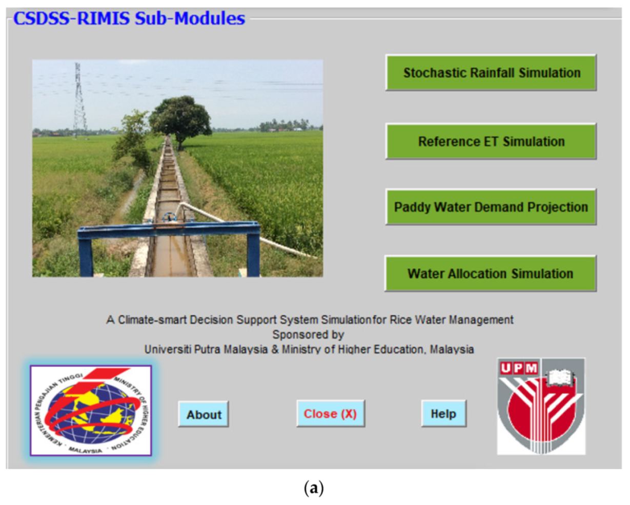
2.1. Location and Field Investigation

The 18,000 ha Northwest Selangor Irrigation Scheme (NSRIS) is situated at 101.18° N latitude and 3.45° E longitude in the state of Selangor, Malaysia (Figure 1). The irrigation scheme plays an important role to meet demand of staple food rice. According to Agrofood Statistics [34], Malaysians consume 80 kg of rice per person per year that covers approximately 26% of the total caloric intake per day. The country has achieved 60% to 70% self-sufficiency level (SSL) for rice production locally, and the rest is imported primarily from Thailand, Vietnam, and Pakistan. Therefore, assessing the impact of climate change on rice productivity of NSRIS is worthwhile to understand the potential intervention in achieving SSL for rice production in the country and to review the performance of the paddy and rice industry. The average yield of rice in NSRIS is 5.8 t/ha, and a sustaining growth in rice production is needed to achieve the SSL.
A Parshall RBC flume with a MJK EXPERT™ 7060 Hydrostatic Water Level Sensor (irrigation flow rate), drainage flow with MJK EXPERT™ 7060 Hydrostatic Water Level Sensor, micro-lysimeters, rain gauge, and eWater level sensor (EXPERT™ 700D Level Transmitter) were installed in the experimental paddy field (Figure 2) for auditing water balance components of the paddy field. Several field staff gauges were installed in the field to measure fluctuating field water levels with an eWater level sensor.
MJK Expert™ 7060 is ideal for monitoring and measuring water levels in tanks, reservoirs and pumping stations. Expert™ 7060 has both an adjustable zero-point and measuring range, as well as a 4–20 mA output signal. Using a standard USB interface and a laptop, the service transmitter can be programmed on-site to the required measuring range. This is done through RS 485 functions via ModBus protocol. Expert™ 700D has an adjustable measuring range of 0–100 m and a very accurate temperature measurement range of −20 °C to 80 °C.

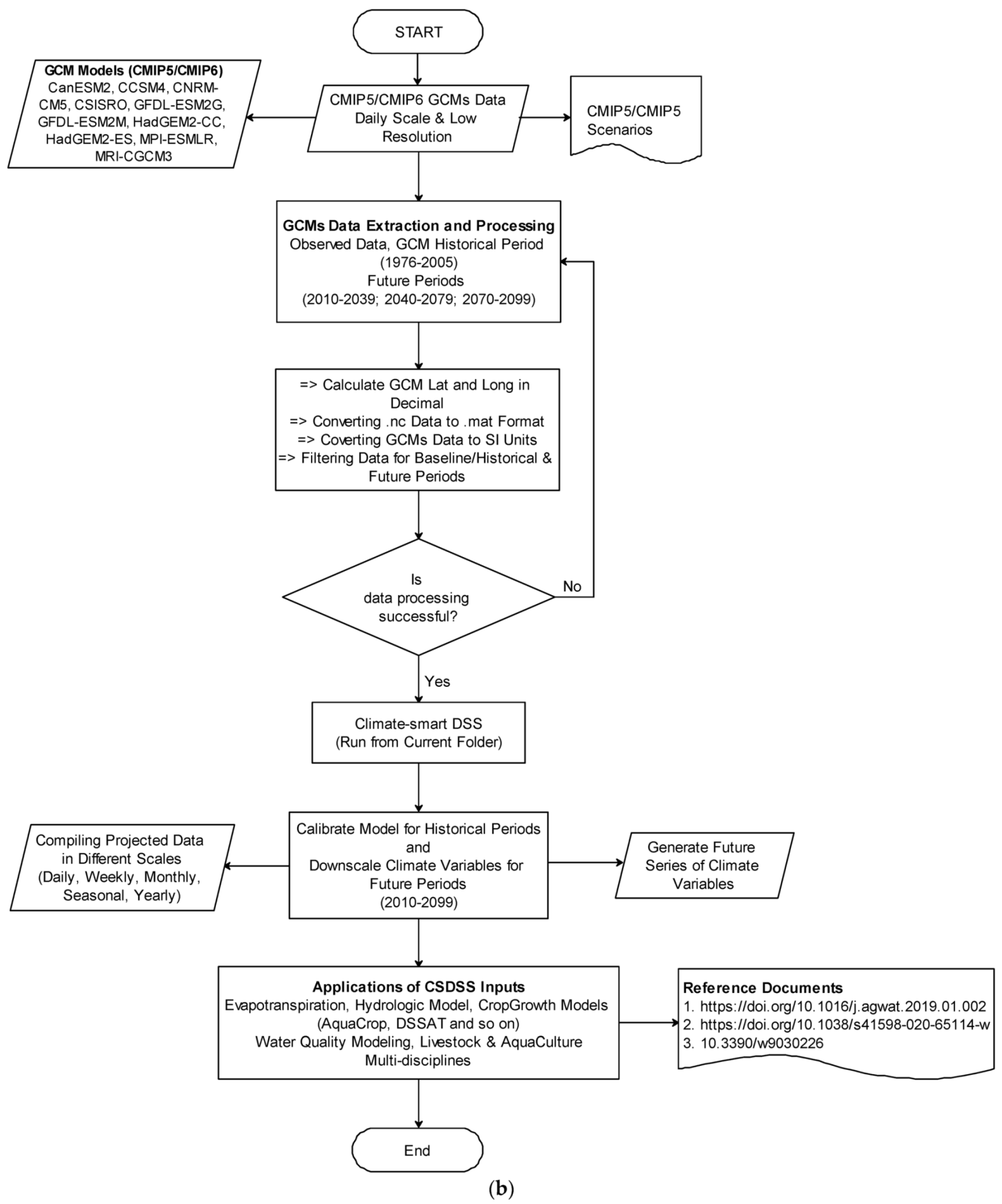
2.2. Climate Data and Downscaling Climate Variables

The daily rainfall, solar radiation, maximum temperature, and minimum temperature of two meteorological stations and six rain gauge stations, distributed in the Northwest Selangor, were obtained from Hydrology Division and Malaysian Meteorological Department (MMD). Daily climate variables for 10 Global Climate Models (GCMs) were downloaded from CMIP5 (Coupled Model Intercomparison Project, https://esgf-node.llnl.gov/search/cmip5/, accessed on 21 October 2021) for the base period of 1976–2005 and future period of 2010–2099. The climate variables were then downscaled using an interactive Climate-Smart Decision Support System (CSDSS) tool [35], which comprises an ensemble of 10 GCMs as shown in Figure 3. To simulate GCM scenarios at the local scale, statistical downscaling methods have been introduced by utilising statistical relationships between model output climate variables and historical climate variables. The relationship between the coarse-scale patterns and the local weather must remain stationary during downscaling. The CSDSS graphical user-interface simulates climate data instantly on daily and monthly time-series, and displays the data in tables and graphs.
The MATLAB Graphics User Interface Development Environment (GUIDE) is used to develop the user-friendly interface. The user interface is mouse-driven and associated with pop-up windows, pull-down menus, and command button controls. MATLAB’s computational power makes it ideal for climate change studies, which requires large amounts of data manipulation, extraction, processing, and computations. Many built-in computational functions and data visualisations are available in it. MATLAB programming codes were written for the GCMs data under the three RCP scenarios (RCP4.5, RCP6.0, and RCP8.5). New climate scenarios and/or GCMs can be easily added or updated to the MATLAB database through an independent executable module and the large amount of GCMs data stored in the database. Figure 3b illustrates the steps followed in simulating daily climate sequences. The CSDSS can be used in different Meteorological stations/regions/basins by altering CMIP5 (https://esgf-node.llnl.gov/search/cmip5/)/CMIP6 (https://esgf-node.llnl.gov/search/cmip6/, accessed on 21 October 2021) GCMs data. To run downscaling model, CSDSS requires observed climate data for a particular location/station. CSDSS was successfully used to downscale climate variables (Tmax, Tmin, rainfall, relative humidity, wind speed, solar radiation, and potential evapotranspiration) and simulate the hydrologic response of the Kurau River Basin for determining inflow patterns of the Bukit Merah Reservoir (https://doi.org/10.1038/s41598-020-65114-w, accessed on 21 October 2021).

2.3. AquaCrop Model

2.3.1. Model Description

The AquaCrop model describes how crops and waterways interact in the soil-crop-atmosphere system. It requires inputs on local climate data, crop characteristics and management practices to run simulation [36]. AquaCrop model calculates actual crop evapotranspiration (ETc) and represents it into transpiration (T) and evaporation (E) in proportion to the covered and uncovered soil surface based on the daily soil-water balance. A normalised crop-water productivity (WP*) model is used to estimate the crop’s biomass production and the ratio of transpiration to evapotranspiration (T/ETc) during crop-growing periods [17].

2.3.2. Model Calibration

The AquaCrop model was calibrated using field experimental data of two consecutive rice seasons (off-season and main season) in 2017. Calibrated parameters of the AquaCrop 6.0 model are presented in Table 1. The conservative parameters in the model were adopted based on recommendation [37].

2.3.3. Model Validation Criteria

Root-Mean-Square Error (RMSE), Mean Absolute Error (MAE), Percent Measured Error (PME) and Index of Agreement (d) were used to validate the AquaCrop model. RMSE measures the difference between the model-predicted values and the observed values of a parameter. The individual differences, called residuals, are aggregated into a single measure of predictive power by the RMSE. It measures the magnitude of discrepancy between two sets of data and is a useful metric for comparing the accuracy of different models in the context of comparing prediction errors. RMSE is expressed as:
RMSE = i = 1 n   ( O i   S i ) 2 n
where Si is the simulated rice yield, Oi is the observed rice yield, and n is the number of observations.
The mean absolute error (MAE) of a test sample is expressed by the weighted average of all absolute differences between the prediction and observations. Both RMSE and MAE express average model prediction error and can range from 0 to infinity; they are indifferent to the direction of errors. MAE is expressed as:
MAE = ( S i     O i ) O i  
Bias in prediction is indicated by a prediction error (PE) in terms of the total difference between the measured and simulated data points. It is determined by:
PE = i = 1 n ( S i O i ) n  
The index of agreement (d) is a standardised measure of model prediction error that varies from 0 to 1. This index represents the ratio of mean-square error and potential error. A value of 1 indicates perfect agreement, while a value of 0 denotes no agreement at all. Due to squared differences, the index of agreement is overly sensitive to extreme values in the observed and simulated means and variances. The index of agreement, d, is expressed as:
d = 1 i = 1 n ( O i S i ) 2 i = 1 n ( / S i Ō / + / O i Ō / ) 2
where Ō is the average rice yield.

2.4. Simulation for Future (2010–2099)

2.4.1. Crop Yield

Rice yields were simulated under climate change conditions for RCP4.5, RCP6.0, and RCP8.5 emission scenarios using the calibrated AquaCrop model. Climate data and CO2 concentration were varied in order to simulate future climate conditions, while other input parameters, such as soil, crop, and management practices were kept unchanged over time. We evaluated the impacts of climate change by comparing the baseline yields (1990s: 1976–2005) with simulated yields for three future periods (2010–2039, 2040–2069, 2070–2099).

2.4.2. Actual Crop Evapotranspiration and Crop Coefficient

Actual crop evapotranspiration, ETc (mm day−1) is computed by multiplying reference evapotranspiration (ETo, mm day−1) by a crop coefficient (Kc) at different growth stages of rice, as
E T c   = K c   ×   E T o .
The FAO Penman–Monteith model, used for estimating ETo [38], is expressed by
ET o   t , s = 0 . 408 ( R n G ) + γ 900 T + 273 u 2 ( e s e a ) + 2 ( 1 + 0 . 34 u 2 )
For details of the variables and coefficients of the Penman–Monteith model, the readers are referred to [38].

2.4.3. Water Productivity

Water productivity (WP) is the amount of water required to produce yield. Several indices of WP terms are expressed as:
W P I i r r = Yied IR + RF
W P I I R + E R = Yied IR + RF eff  
W P I I R = Yied IR
W P I E T c = Y i e l d E T c
In Equations (7)–(10), WPI is the water productivity index (fraction), IR is the irrigation water requirement (m3), RF is rainfall (m3), RFeff is the effective rainfall (m3), and ETc is the actual crop evapotranspiration (m3); the yield of rice is expressed in kilograms.

3. Results and Discussion

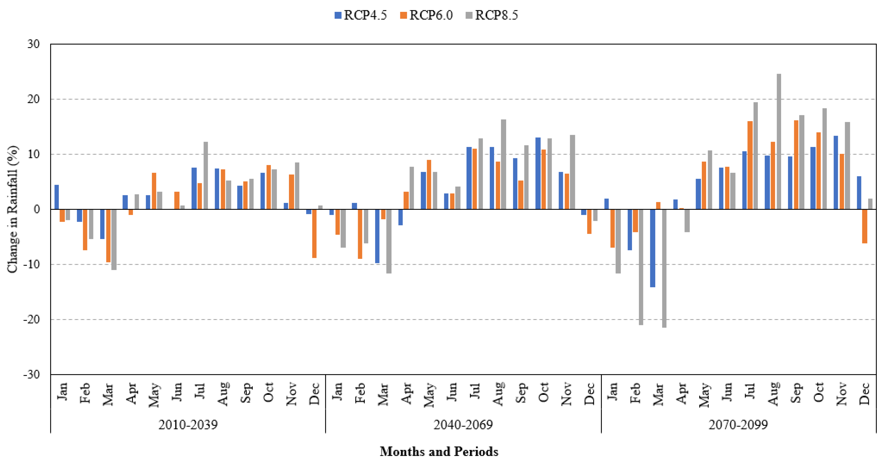
3.1. Future Climate Change

The climate forecasts (Table 2) divulge that the temperature (both minimum and maximum) in the agro-hydrological Bernam River Basin will increase in future (2010–2099). The predicted annual rainfall is 5.8% more compared to its baseline (1990s: 1976–2005) magnitude for the three emission scenarios (RCP4.5, RCP6.0, and RCP8.5).
In the long-term, the overall rainfall is expected to increase in the main season but decrease in the off-season for the three future periods. However, the changes in monthly total rainfall will differ considerably with the GCMs and RCP emission scenarios, as illustrated in Figure 4. These trends in rainfall will influence irrigation requirement, and hence the water productivity of rice. The increase in rainfall in the main season will also compensate, to some extent, the effects of temperature on rice production.

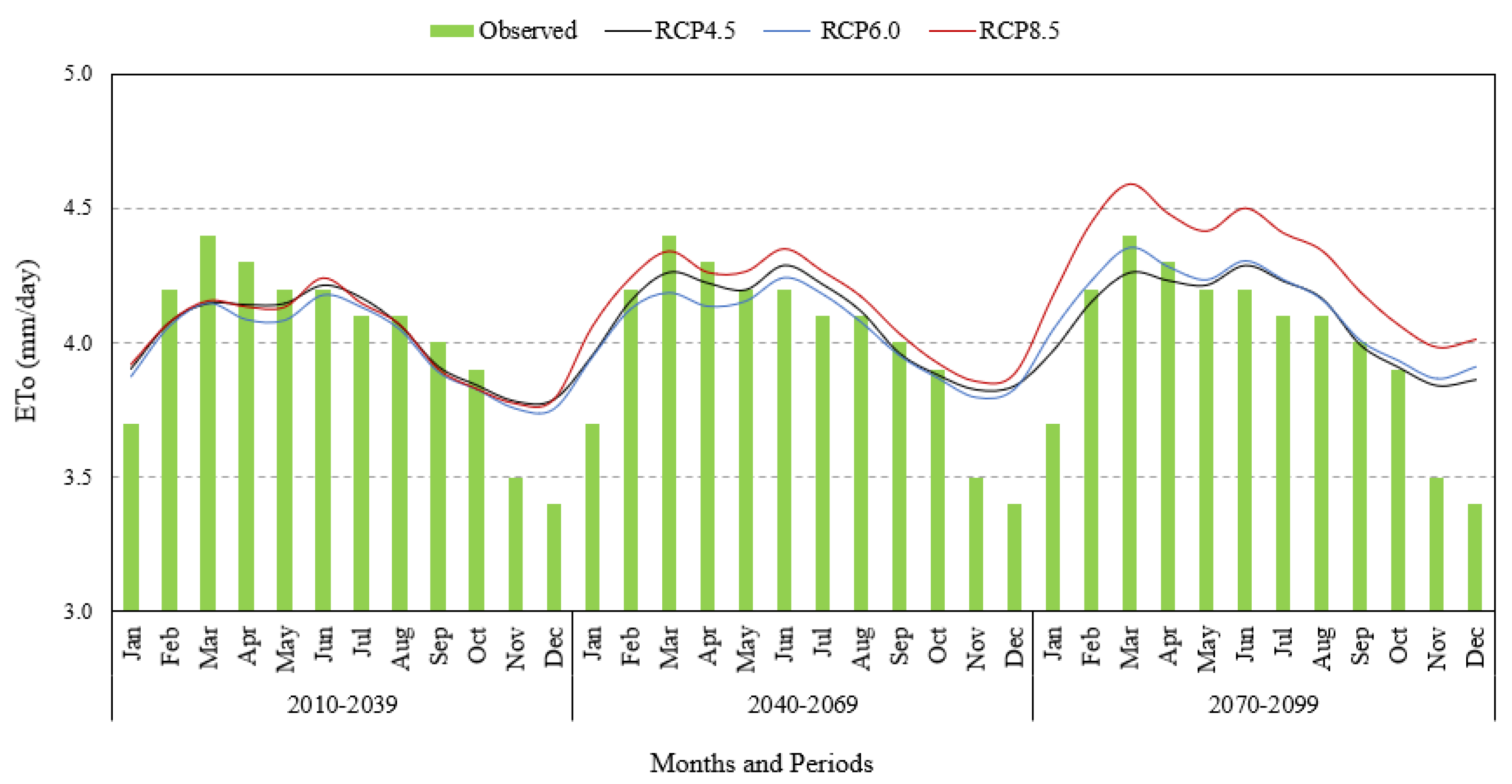
3.2. Reference Evapotranspiration

The monthly variation of reference evapotranspiration, ETo, during the year 2017, and the projected ETo for the three future periods are illustrated in Figure 5. In the off-season, the highest mean ETo is predicted to be 4.6 mm day−1 on the 21 of March during the 2080s under RCP8.5, and the lowest mean ETo is 3.67 mm day−1 predicted on 1 January during 2020s under RCP6.0. In the main season, the highest mean ETo (4.5 mm day−1) is on 25 July during the 2080s under RCP8.5, and the lowest mean ETo (3.58 mm day−1) is on 14 October during the 2050s under RCP6.0. The predicted ETo under RCP8.5 is much larger than that under the other RCP scenarios during the period of 2070–2099.

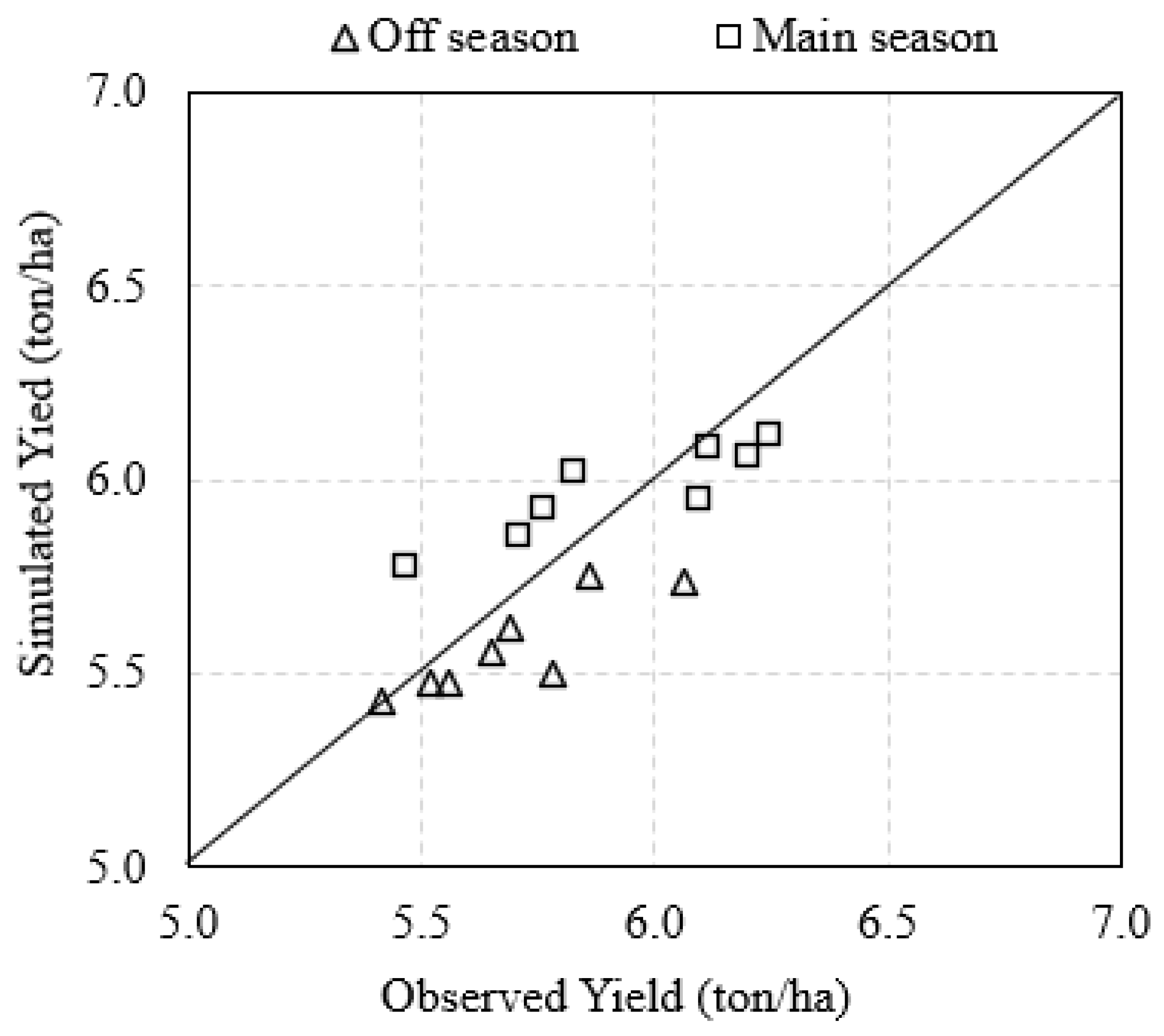
3.3. Performance of AquaCrop Model

The predicted rice yields during calibration were slightly higher compared to the observed yields of 5500 kg ha1 in the off-season and 5850 kg ha1 in the main season; the variation in yield in the corresponding season was 1.0% and 3.1%. However, the model performed fairly well in predicting the yields during the validation period (2009 to 2016). Indeed, reliable and high-quality experimental data can enhance the performance of calibration and validation of crop parameters in diverse environments. The model, however, effectively simulated rice yields in both crop seasons. As shown in Figure 6, the predicted and observed yields of rice are in good agreement during the validation period for both crop seasons. For the off-season, the root-mean-square error (RMSE), mean absolute error (MAE), prediction error (PE), and index of agreement (d) are 0.173, 0.157, −0.31 to 5.6 and 0.78, respectively. The corresponding indicators for the main season are 0.167, 0.127, −5.6 to 2.34 and 0.734. The performance indicators (RMSE, MAE, PE, and d) of the model indicating a yield difference of only 0.74% to 2.9% demonstrate that the AquaCrop model has good potential to accurately predict rice yields in Malaysia.
The climate variables, by influencing the growth and development phases of rice, contributed increasing the simulated rice yield over time. Despite rising temperatures in the study area, there are still opportunities to increase rice yields because of favorable rainfall patterns. Model validation results indicate that AquaCrop model can simulate potential rice yields within reasonable accuracy. Only small fluctuations were observed in the simulated rice yields during model validation. The model could accurately predict the growth and yield of rice under different water management strategies. Therefore, AquaCrop model integrated with CSDSSS can promote development of adaptation strategies for the irrigation districts.

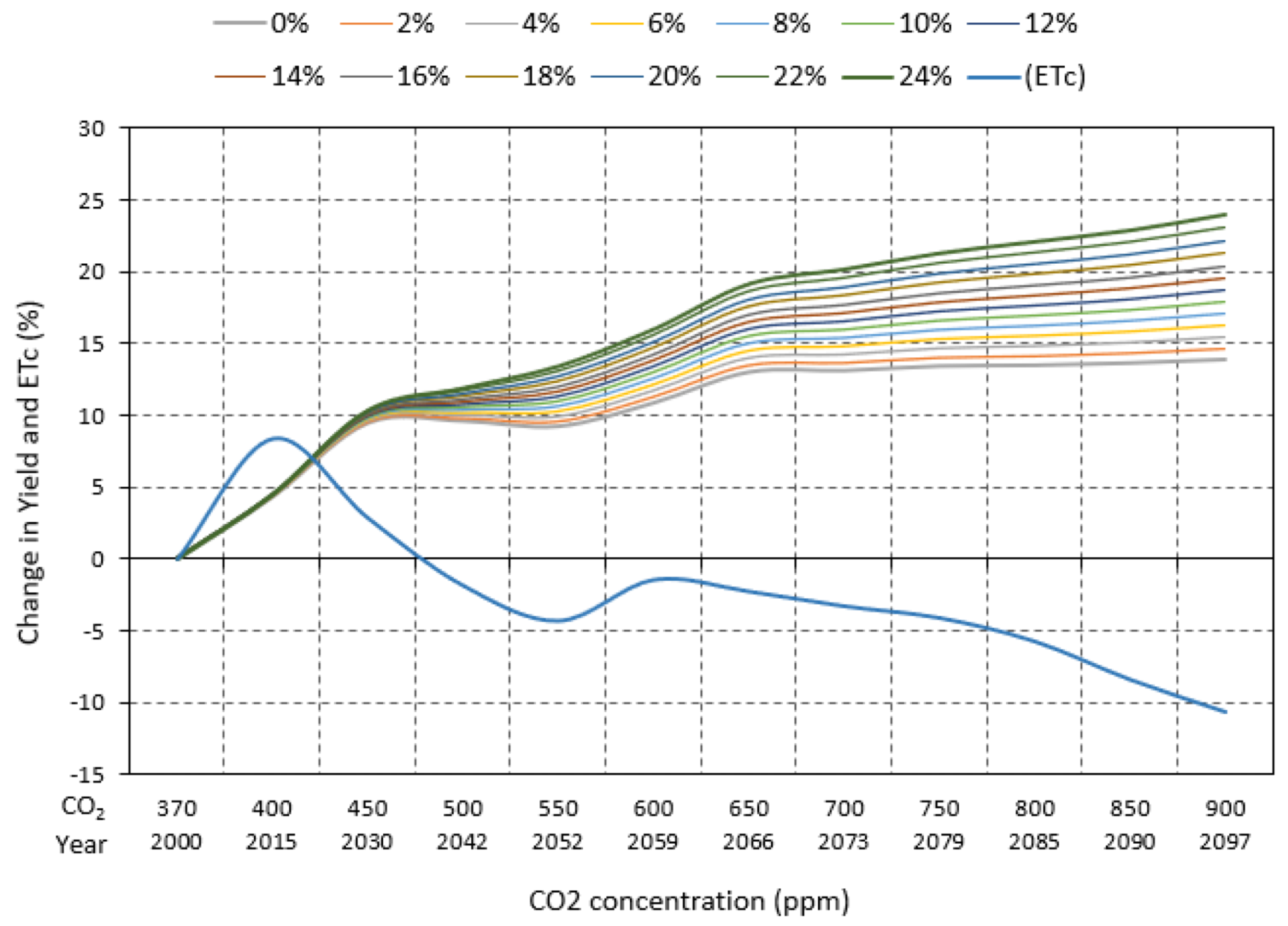
3.4. Effect of CO2 on Yield and ETc under Projected Climate Change

The sink strength of rice and its responsiveness to CO2, specifically at high concentrations exceeding 550 ppm, vary between 0 and 22% [39]. Thus, the AquaCrop model was run based on this range of crop sink strength to predict the future yield and yield variation of rice associated with the sink strength. Despite the increasing trend of temperature in the study area, the rising CO2 concentration exerts positive impacts on the yield and water usage of rice crop. The predicted results indicate that rice yield would increase by 13–24% and crop-water use would decrease by 11% by the end of the current century, thus boosting local irrigation water availability and crop-water productivity (Figure 7).
According to current projections [40], CO2 concentrations are expected to reach 500–1000 ppm by 2100. With rising CO2 concentration, plants can uphold high photosynthetic rates at low stomatal conductance. Across a variety of Free-Air Carbon dioxide Enrichment (FACE) experiments, water stomatal conductance has been found to decrease by 22% under conditions of increased CO2 exposure [41]. Although the overall effect of CO2 is expected to reduce plant-water use, the magnitude will depend on how it affects other factors, like the size of the plant, its morphology, and the temperature of the leaf. In the FACE experiments, water use by the plant drops by 5–20% with elevated levels of CO2 concentration. Increasing CO2 levels also have the potential to modify the hydrological cycle of the ecosystems, since the soil moisture and runoff increase [42].

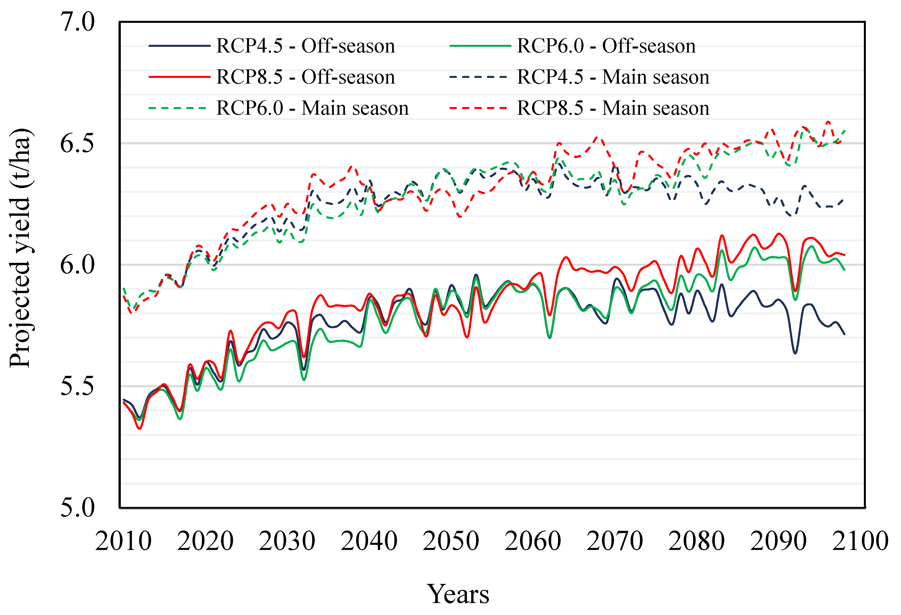
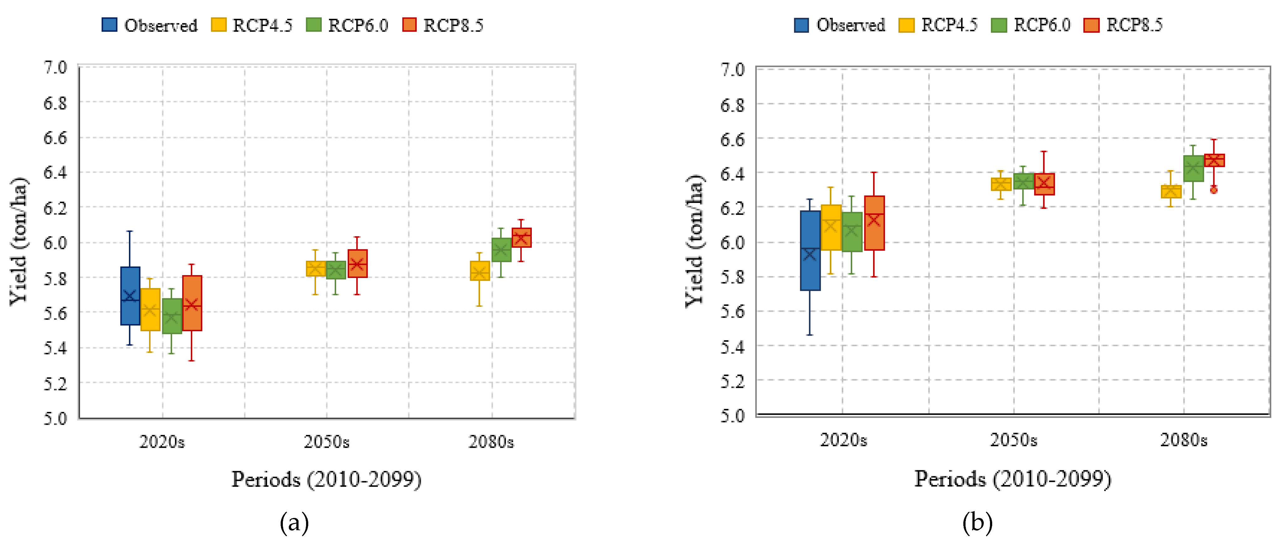
3.5. Projected Yield

The predicted rice yields show increasing trends in both crop seasons (Figure 8), the increase being 9.8% to 18.8% under the three RCP emission scenarios, with a strong increase in the 2020s, but a moderate increase in the 2080s. The projected rice yield is 5.8–6.4 t/ha in 2020s, 6.2–6.5 t/ha in 2050s, and 6.2–6.5 t/ha in 2080s in the main season, and 5.3–5.8 t/ha in 2020s, 5.7–6.0 t/ha in 2050s, and 5.6–6.1 t/ha in 2080s in the off-season (Figure 9). Therefore, it is anticipated that rice production in Malaysia will benefit from the changing climate in the future. However, some studies [43,44] predicted increasing or decreasing trends of crop yields in Asia in response to CO2 concentrations.
The responses of crop yield and crop-water productivity to future climate change need to be quantified in order to circumvent or lessen the adverse impacts of climate change. Dang (2000) determined suitable times for broadcasting rice crops and highlighted that a shift in the rice broadcasting calendar compared to the baseline can be an effective solution to minimize the negative impacts of weather factors, as well as contribute increasing yield [45]. The projected results of our study indicate that, compared to the previous decade, the yield rice will have a encouraging trend by 2040, ranging from −0.02% to 19.85% during the main season and −2.77% to 7.41% during the off-season. However, while the yield of rice is expected to rise in some areas, other areas are anticipated to have adverse effects [46].

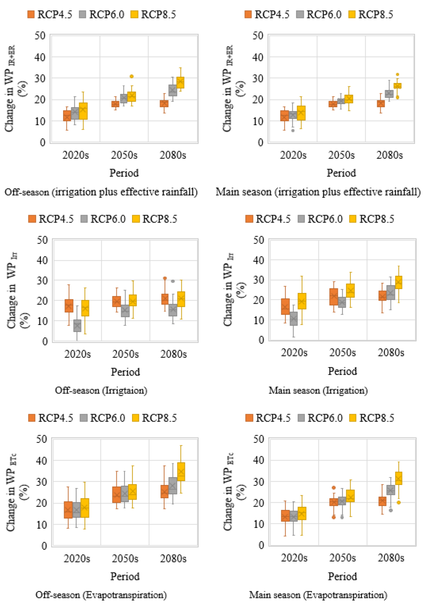
3.6. Projected Water Productivity of Rice

Crop-water productivity is a ratio of crop yield to the amount of water required to produce that yield. The quantity of water can be the total water input (irrigation plus effective rainfall, IR + ER) or applied irrigation (Irr) or actual crop evapotranspiration (ETc). The variation of predicted water productivity, WP, of rice over different time periods is illustrated in Figure 10. WP is 0.46, 0.60, and 1.02 kg m−3 during the baseline period when calculated based on (IR + ER), Irr and ETc, respectively in the off-season. WP for the corresponding base in the main season is 0.49, 0.63, and 1.08 kg m−3. The projected WP follows increasing trends under the three RCP emission scenarios over the future periods for both crop seasons. The WP of rice will likely be higher during the main season compared to the off-season; the difference is significant when WP is estimated based on applied irrigation, Irr. The WP will increase by 8% during the 2050s under RCP4.5 and 13% during the 2080s under RCP6.0 and RCP8.4 emission scenarios. Since increasing rainfall reduces irrigation requirements of the crop, the large increase in WP will be attributed to the increase in rainfall in the main season. The largest increase in WPETc is projected under the RCP8.5 emission scenario in both crop seasons during the 2080s, since the projected increase in effective rainfall and CO2 concentration will likely reduce crop evapotranspiration and improve crop-production efficiency. A shortened growth period of rice under increasing temperature will also contribute reducing crop evapotranspiration. Furthermore, reduced stomatal conductance under elevated CO2 will reduce transpiration per unit leaf area [47]. The expected role of elevated CO2 in reducing evapotranspiration and increasing water productivity for rice is consistent with other studies [48,49]. Thus, the FAO AquaCrop model can be used to reliably simulate the effects of various irrigation management strategies for improving the water productivity of rice.

4. Conclusions

Downscaled ensemble climate variables using Climate-smart Decision Support System (CSDSS) together with field experimental data and recommended model parameters were used as inputs to AquaCrop model, and rice yield and water productivity (WP) indicators were simulated for 2010–2039, 2040–2069, and 2070–2099 future periods relative to the 1976–2005 base period in Malaysia. The projected increasing trend of the maximum and minimum temperatures in two crop seasons (off-season: January–June and main season: July–December), increasing rainfall during the main season, and decreasing rainfall during the off-season will likely exert multi-layered impacts on rice production and WP. The simulated increasing trend of WP with increasing CO2 concentration, temperature, and rainfall under RCP4.5, RCP6.0, and RCP8.5 emission scenarios indicates an improved synergy for rice growth under the projected water-heat-carbon status. However, there remains some degree of uncertainty in the magnitude of projected WP, since the AquaCrop model, to some extent, systematically overestimated rice production. The reason of overestimation might be the highly daily variable and short-period rainfall patterns, and not accounting for the impacts of climate change on agronomical practices (e.g., irrigation, drainage, weeding, pest control, and fertilizer application). Despite this weakness, the proposed model would fairly predict rice yields under the likely evolved future climate change and different water regimes. The information on WP would help to devise a strategic water management plan during periods of both shortage and excess of water as currently occurring during the two rice-growing seasons in the Northwest Selangor Irrigation Scheme. The model can be adopted in planning crop and water management to increase WP in any region, especially in areas with water shortage. The AquaCrop model can be used as a decision support tool to boost water productivity. However, development of a user interface to access the information interactively will enhance decision-making, especially in complex environments, for adaptation of the AquaCrop model.

Author Contributions

Conceptualization, M.R.K.; methodology, A.A.H. & M.R.K.; software, A.A.H.; validation, A.A.H. and M.R.K.; formal analysis, A.A.H. & M.R.K.; investigation, A.A.H.; resources, M.A.M.Z. & B.M.R.; data curation, A.A.H.; writing—original draft preparation, A.A.H. & M.R.K.; writing—review and editing, M.A.M. & M.R.K.; visualization, A.A.H.; supervision, M.R.K. & M.A.M.Z.; project administration, M.A.M.Z. & B.M.R.; funding acquisition, M.R.K., M.A.M.Z. & B.M.R. All authors have read and agreed to the published version of the manuscript.

Funding

Geran Putra Berimpak, Universiti Putra Malaysia & No: 9678600.

Institutional Review Board Statement

Not applicable.

Informed Consent Statement

Not applicable.

Data Availability Statement

Not applicable.

Acknowledgments

We acknowledge Universiti Putra Malaysia for financial support from Putra Grant No: 9678600. The authors thank Dirk Raes for his scholarly scientific advice on the sink effect on rice production.

Conflicts of Interest

The authors declare no conflict of interest in publishing this research.

References

  1. Gitz, V.; Meybeck, A. Climate change and food security: Risks and responses. Food Agric. Organ. United Nations Rep. 2016, 110, 1–98. [Google Scholar]
  2. Lal, R.; Uphoff, N.; Stewart, B.A.; Hansen, D.O. Climate Change and Global Food Security; CRC Press: Boca Raton, FL, USA, 2005; pp. 1–744. [Google Scholar]
  3. Masson-Delmotte, V.P.; Zhai, H.-O.; Pörtner, D.; Roberts, J.; Skea, P.R.; Shukla, A.; Pirani, W.; Moufouma-Okia, C.; Péan, R.P. (Eds.) IPCC: Summary for Policymakers. In Global Warming of 1.5 °c. An IPCC Special Report on the Impacts of Global Warming of 1.5 °C above Pre-Industrial Levels and Related Global Greenhouse Gas Emission Pathways, in the Context of Strengthening the Global Response to the Threat of Climate Change, Sustainable Development, and Efforts to Eradicate Poverty; Intergovernmental Panel on Climate Change: Geneva, Switzerland, 2018; pp. 31–116. [Google Scholar]
  4. Oki, T.; Kanae, S. Global Hydrological Cycles and Freshwater Resources Fresh water. Science 2006, 313, 1068–1073. [Google Scholar] [CrossRef] [Green Version]
  5. Zaki, M.M.M.; Ercan, A.; Ishida, K.; Kavvas, L.M.; Chen, Z.Q.; Jang, H.Q. Impacts of Climate Change on the Hydro-Climate of Peninsular Malaysia. Water 2019, 11, 1798. [Google Scholar]
  6. Fatimah, K. Evaluation of Agricultural Subsidies and the Welfare of Farmers; Malaysia Agricultural Subsidies Report 2018; IDEAS Policy Research Berhad: Kuala Lumpur, Malaysia, 2018; pp. 1–64. [Google Scholar]
  7. Lautze, J. Key Concepts in Water Resource Management: A Review and Critical Evaluation; Earthscan. (Earthscan Water Text); Routledge: New York, NY, USA, 2014; ISBN 0203005813. [Google Scholar]
  8. Descheemaeker, K.; Bunting, S.W.; Bindraban, P.; Muthuri, C.; Molden, D.; Beveridge, M.; van Brakel, M.; Herrero, M.; Clement, F.; Boelee, E.; et al. Increasing water productivity in agriculture. In Managing Water and Agroecosystems for Food Security; Boelee, E., Ed.; CABI Publishing: Wallingford, UK, 2013; ISBN 9781780640884. [Google Scholar]
  9. Cai, X.; Rosegrant, M.W. World water productivity: Current situation and future options. In Water Productivity in Agriculture: Limits and Opportunities for Improvement; Kijne, J.W., Barker, R., Molden, D., Eds.; CABI: Wallingford, UK; International Water Management Institute (IWMI): Colombo, Sri Lanka, 2003; pp. 163–178. [Google Scholar]
  10. Mojid, M.A.; Mainuddin, M. Water-saving agricultural technologies: Regional hydrology outcomes and knowledge gaps in the eastern gangetic plains-a review. Water 2021, 13, 636. [Google Scholar] [CrossRef]
  11. Farshi, A.; Feyen, J.; Belmans, C.; Wijngaert, K.D. Modelling of yield of winter wheat as a function of soil water availability. Agric. Water Manag. 1987, 12, 323–339. [Google Scholar] [CrossRef]
  12. Pang, X.P.; Letey, J. Development and Evaluation of ENVIRO-GRO, an Integrated Water, Salinity, and Nitrogen Model. Soil Sci. Soc. Am. J. 1998, 62, 1418–1427. [Google Scholar] [CrossRef]
  13. Pirmoradian, N.; Sepaskhah, A.R. A very simple model for yield prediction of rice under different water and nitrogen applications. Biosyst. Eng. 2006, 93, 25–34. [Google Scholar] [CrossRef]
  14. Zand-Parsa, S.; Sepaskhah, A.R.; Ronaghi, A. Development and evaluation of integrated water and nitrogen model for maize. Agric. Water Manag. 2006, 81, 227–256. [Google Scholar] [CrossRef]
  15. Araya, A.; Habtu, S.; Hadgu, K.M.; Kebede, A.; Dejene, T. Test of AquaCrop model in simulating biomass and yield of water deficient and irrigated barley (Hordeum vulgare). Agric. Water Manag. 2010, 97, 1838–1846. [Google Scholar] [CrossRef]
  16. Boonwichai, S.; Shrestha, S.; Babel, M.S.; Weesakul, S.; Datta, A. Climate change impacts on irrigation water requirement, crop-water productivity and rice yield in the Songkhram River Basin, Thailand. J. Clean. Prod. 2018, 198, 1157–1164. [Google Scholar] [CrossRef]
  17. Hsiao, T.C.; Heng, L.; Steduto, P.; Rojas-Lara, B.; Raes, D.; Fereres, E. Aquacrop-The FAO crop model to simulate yield response to water: III. Parameterization and testing for maize. Agron. J. 2014, 101, 448–459. [Google Scholar] [CrossRef]
  18. Mkhabela, M.S.; Bullock, P.R. Performance of the FAO-AquaCrop model for wheat grain yield and soil moisture simulation in Western Canada. Agric. Water Manag. 2012, 110, 16–24. [Google Scholar] [CrossRef]
  19. Steduto, P.; Hsiao, T.C.; Raes, D.; Fereres, E. AquaCrop-the FAO crop model to simulate yield response to water: I. concepts and underlying principles. Agron. J. 2009, 101, 426–437. [Google Scholar] [CrossRef] [Green Version]
  20. Zeleke, K.T.; Luckett, D.; Cowley, R. Calibration and testing of the FAO-AquaCrop model for canola. Agron. J. 2011, 103, 1610–1618. [Google Scholar] [CrossRef]
  21. Zhao, J.; Han, T.; Wang, C.; Jia, H.; Worqlul, A.W.; Norelli, N.; Zeng, Z.; Chu, Q. Optimizing irrigation strategies to synchronously improve the yield and water productivity of winter wheat under interannual precipitation variability in the North China Plain. Agric. Water Manag. 2020, 240, 106298. [Google Scholar] [CrossRef]
  22. Tan, B.T.; Fam, P.S.; Firdaus, R.B.R.; Tan, M.L.; Gunaratne, M.S. Impact of Climate Change on Rice Yield in Malaysia: A Panel Data Analysis. Agriculture 2021, 11, 569. [Google Scholar] [CrossRef]
  23. Le Loh, J.; Tangang, F.; Juneng, L.; Hein, D.; Lee, D.I. Projected rainfall and temperature changes over Malaysia at the end of the 21st century based on PRECIS modelling system. Asia-Pac. J. Atmos. Sci. 2016, 52, 191–208. [Google Scholar] [CrossRef]
  24. Yinhong, K.; Shahbaz, K.; Xiaoyi, M. Climate change impacts on crop yield, crop-water productivity and food security—A review. Prog. Nat. Sci. 2009, 19, 1664–1674. [Google Scholar]
  25. Carter, T.R.; Hulme, M.; Viner, D. Representing uncertainty in climate change scenarios and impact studies. In Proceedings of the Helsinki Workshop, Norwich, UK, 14–16 April 1999; ECLAT-2 Report No. 1. p. 130. [Google Scholar]
  26. Liu, Q.; Jun, N.; Sivakumar, B.; Ding, R.; Li, S. Accessing future crop yield and crop-water productivity over the Heihe River basin in northwest China under a changing climate. Geosci. Lett. 2021, 8, 2. [Google Scholar] [CrossRef]
  27. Raes, D.; Steduto, P.; Hsiao, T.C.; Fereres, E. AquaCrop—the FAO crop model to simulate yield response to water: II. main algorithm and software description. Agron. J. 2009, 101, 438–477. [Google Scholar] [CrossRef] [Green Version]
  28. Saadati, Z.; Pirmoradian, N.; Rezaei, M. Calibration and evaluation of AquaCrop model in rice growth simulation under diferent irrigation managements. In Proceedings of the 21st International Congress on Irrigation and Drainage, Tehran, Iran, 15–23 October 2011; pp. 589–600. [Google Scholar]
  29. Lin, L.; Zhang, B.; Xiong, L. Evaluating yield response of paddy rice to irrigation and soil management with application of the AquaCrop model. Trans ASABE 2012, 55, 839–848. [Google Scholar] [CrossRef]
  30. Shrestha, N.; Raes, D.; Vanuytrecht, E.; Sah, S.K. Cereal yield stabilization in Terai (Nepal) by water and soil fertility management modeling. Agric. Water Manag. 2013, 122, 53–62. [Google Scholar] [CrossRef]
  31. Maniruzzaman, M.; Talukder, M.S.U.; Khan, M.H.; Biswas, J.C.; Nemes, A. Validation of the AquaCrop model for irrigated rice production under varied water regimes in Bangladesh. Agric. Water Manag. 2015, 159, 331–340. [Google Scholar] [CrossRef]
  32. Sandhu, S.S.; Mahal, S.S.; Kaur, P. Calibration, validation and application of AquaCrop model in irrigation scheduling for rice under northwest India. J. Appl. Nat. Sci. 2015, 7, 691–699. [Google Scholar] [CrossRef] [Green Version]
  33. Kontgis, C.; Schneider, A.; Ozdogan, M.; Kucharik, C.; Tri, V.P.D.; Duc, N.H.; Schatz, J. Climate change impacts on rice productivity in the Mekong River Delta. Appl. Geogr. 2019, 102, 71–83. [Google Scholar] [CrossRef]
  34. Kruijt, B.; Witte, J.P.M.; Jacobs, C.M.J.; Kroon, T. Effects of rising atmospheric CO2 on evapotranspiration and soil moisture: A practical approach for the Netherlands. J. Hydrol. 2008, 349, 257–267. [Google Scholar] [CrossRef]
  35. MOA. Agrofood Statistics 2016; Ministry of Agriculture, The Government of Malaysia: Putrajaya, Malaysia, 2016.
  36. Rowshon, M.K.; Dlamini, N.S.; Mojid, M.A.; Adib, M.N.M.; Amin, M.S.M.; Lai, S.H. Modeling climate-smart decision support system (CSDSS) for analyzing water demand of a large-scale rice irrigation scheme. Agric. Water Manag. 2019, 216, 138–152. [Google Scholar] [CrossRef]
  37. Raes, D.; Steduto, P.; Hsiao, T.C.; Fereres, E. Calculation Procedures; AquaCrop Version 6.0–6.1; Food and Agriculture Organization of the United Nations: Rome, Italy, 2018; Chapter 3; p. 125. [Google Scholar]
  38. Allen, R.G.; Pereira, L.S.; Raes, D.; Smith, M. Crop Evapotranspiration Guidelines for Computing Crop Water Requirements; FAO—Food and Agriculture Organization of the United Nation: Rome, Italy, 1998; ISBN 9251042195. [Google Scholar]
  39. Vanuytrecht, E.; Raes, D.; Willems, P. Considering sink strength to model crop production under elevated atmospheric CO2. Agric. For. Meteorol. 2011, 151, 1753–1762. [Google Scholar] [CrossRef]
  40. IPCC. Climate Change 2007: The Physical Science Basis. Contribution of Working Group I to the Fourth Assessment Report of the Intergovernmental Panel on Climate Change; Cambridge University Press: Cambridge, UK, 2007. [Google Scholar]
  41. Ainsworth, E.A.; Rogers, A. The response of photosynthesis and stomatal conductance to rising (CO2): Mechanisms and environmental interactions. Plant Cell Environ. 2007, 30, 258–270. [Google Scholar] [CrossRef]
  42. Leakey, A.D.; Ainsworth, E.A.; Bernacchi, C.J.; Rogers, A.; Long, S.P.; Ort, D.R. Elevated CO2 effects on plant carbon, nitrogen, and water relations; six important lessons from FACE. J. Exp. Bot. 2009, 60, 2859–2876. [Google Scholar] [CrossRef] [PubMed]
  43. Tesfaye, K.; Zaidi, P.H.; Gbegbelegbe, S.; Boeber, C.; Rahut, D.B.; Getaneh, F.; Seetharam, K.; Erenstein, O.; Stirling, C. Climate change impacts and potential benefits of heat-tolerant maize in South Asia. Theor. Appl. Climatol. 2017, 130, 959–970. [Google Scholar] [CrossRef] [Green Version]
  44. Parry, M.; Canziani, O.; Palutikof, J.; van der Linden, P.; Hanson, C. Climate Change 2007: Impacts, Adaptation and Vulnerability. Contribution of Working Group II to the Fourth Assessment Report of the Intergovernmental Panel on Climate Change Published; Cambridge University Press: Cambridge, UK, 2007; ISBN 9780521880107. [Google Scholar]
  45. Dang, T.A. Shifting crop planting calendar as a climate change adaptation solution for rice cultivation region in the Long Xuyen Quadrilateral of Vietnam. Chil. J. Agric. Res. 2020, 80, 468–477. [Google Scholar]
  46. Wu, S.J.; Chiueh, Y.W.; Ho, C.L.; Chih, T.H. Modeling risk analysis for rice production due to agro-climate change in Taiwan. Paddy Water Environ. 2014, 13, 391–404. [Google Scholar] [CrossRef]
  47. Parry, M.L.; Rosenzweig, C.; Iglesias, A.; Livermore, M.; Fischer, G. Effects of climate change on global food production under SRES emissions and socio-economic scenarios. Glob. Environ. Chang. 2004, 14, 53–67. [Google Scholar] [CrossRef]
  48. Deryng, D.; Elliott, J.; Folberth, C.; Müller, C.; Pugh, T.A.M.; Boote, K.J.; Conway, D.; Ruane, A.C.; Gerten, D.; Jones, J.W.; et al. Regional disparities in the beneficial effects of rising CO2 concentrations on crop-water productivity. Nat. Clim. Chang. 2016, 6, 786–790. [Google Scholar] [CrossRef] [Green Version]
  49. Nechifor, V.; Winning, M. Global crop output and irrigation water requirements under a changing climate. Heliyon 2019, 5, e01266. [Google Scholar] [CrossRef] [PubMed] [Green Version]
Figure 1. Location of the experimental plot in the Northwest Selangor Irrigation Scheme in Malaysia. (a) Rice production in large-scale granaries (Agrofood Statistics, MOA 2016) & (b) Study location.
Applsci 11 11253 g001aApplsci 11 11253 g001b
Figure 2. A view of different equipment installed in a paddy plot. (a) Layout for installed equipment. (b) Experimental paddy plot. (1. Inlet-RBC Parshall Flume, 2. Rain-gauge, 3. Marriott tube, 4. Micro-lysimeter, 5. e-Water level sensor, 6. ETgauge, and 7. Field outlet).
Applsci 11 11253 g002
Figure 3. Downscaling climate variables using Climate-smart DSS. (a) Climate-smart DSS Main window. (b) Flowchart diagram for the downscaling technique.
Applsci 11 11253 g003aApplsci 11 11253 g003b
Figure 4. Projected changes in rainfall during the period of 2010–C2099 under emission scenarios RCP4.5, RCP6.0, and RCP8.5.
Applsci 11 11253 g004
Figure 5. Variation of the projected monthly reference evapotranspiration (ETo) under emission scenarios RCP4.5, RCP6.0 and RCP8.5 over the period of 2010–2099.
Applsci 11 11253 g005
Figure 6. Simulated rice yields for the off-season (January to April) and main season (July to October) versus observed rice yields using AquaCrop model over the period from 2009 to 2016.
Applsci 11 11253 g006
Figure 7. Temporal changes in rice yield and actual crop evapotranspiration (ETc) based on the sink strength and responsiveness of rice to the elevated CO2 concentration.
Applsci 11 11253 g007
Figure 8. Variation of predicted rice yields from 2010 to 2099 under RCP4.5, RCP6.0, and RCP8.5 emission scenarios in the off-season (January to April) and main season (July to October).
Applsci 11 11253 g008
Figure 9. Predicted rice yields under the RCP4.5, RCP6.0, and RCP8.5 emission scenarios in the off-season (January to April) and main season (July to October) in the 2020s, 2050s, and 2080s. (a) predicted off-season (January–April) rice yield and (b) predicted main season (July–October) rice yield.
Applsci 11 11253 g009
Figure 10. Predicted changes in water productivity (WP) of rice based on irrigation plus effective rainfall, irrigation, and actual crop evapotranspiration under RCP4.5, RCP6.0, and RCP8.5 scenarios for the 2020s, 2050s, and 2080s.
Applsci 11 11253 g010
Table 1. Calibrated parameters of the FAO-AquaCrop 6.0 model used in simulating rice yield for the off-season and main season.
Parameter DescriptionValue
Main Season (July to October)Off Season (January to April)
Base temperature (°C)1010
Upper temperature (°C)3030
Initial canopy cover (%)106.5
Time from sowing to emergence (GDD)152117
Maximum canopy coverage (%)9590
Time between sowing and flowering (GDD)13021135
Duration of flowering stage (GDD)136164
Time between sowing and senescence initiation (GDD)14911273
Time between sowing and maturity (GDD)18911681
Effective minimum root depth (m)0.300.30
Effective maximum root depth (m)0.600.55
Normalized water productivity due to ETo and CO2 (g m−2)1516
Harvest index (HIo)4438
Table 2. Projected changes in the maximum temperature (ΔTmax), minimum temperature (ΔTmin), wind speed (ΔWs), rainfall (ΔRF), relative humidity (ΔRH) and CO2 concentration in the Northwest Selangor Irrigation Scheme area.
RCP ScenarioTime PeriodCO2 Concentration (ppm)ΔRF
(%)
ΔTmin (°C)ΔTmax (°C)ΔWs
(m s −1)
ΔRH
(%)
Baseline
1976–2005
369146.3023.9031.501.1079.90
RCP4.52010–20394232.370.720.620.04−0.07
2040–20694954.011.331.190.010.03
2070–20995324.691.691.500.010.03
RCP6.02010–20394181.020.640.550.070.18
2040–20694943.151.211.050.100.18
2070–20996125.781.841.710.070.27
RCP8.52010–20394322.340.790.700.78−0.16
2040–20695724.941.851.750.76−0.25
2070–20997994.733.213.010.85−0.38
Publisher’s Note: MDPI stays neutral with regard to jurisdictional claims in published maps and institutional affiliations.

