1. Introduction
The modeling of electrical devices is, at present, mainly based on the eddy current problem which allows a representative model of the behavior in the low-frequency domain to be obtained. With the advent of power electronics, devices are subject to high-frequency voltage and current stresses that must be taken into account, since this leads to the accelerated aging of insulators. Meanwhile, due to the development of the wide bandgap semiconductors used in the power converters, the frequency of voltage waveforms applied to the winding of electrical devices becomes increasingly high, especially in the case of pulse-width modulation (PWM). Consequently, resistive, capacitive, and even inductive effects should be simultaneously considered.
In the literature, the electrostatic, electrokinetic, and magnetostatic problems are widely used at low frequencies to capture the decoupled capacitive, resistive, and inductive effects, respectively [
1,
2]. When the frequency of the voltage supply applied to windings of electrical devices increases, the electric field in the regions close to the windings cannot be neglected, especially in the case of PWM [
3]. In this case, special attention should be paid to the coupled resistive-capacitive effects. In practice, the electro-quasistatic (EQS) model [
4] is commonly used for fields resulting from high voltage, withstand applications, or microelectronics, since this model is valid when the characteristic length of magnetic phenomena is low with respect to the wavelength [
4,
5]. However, if the skin effect appears on the distribution of the current density in the winding, the coupled resistive-inductive effects have to be taken into account, and so the magneto-quasistatic (MQS) [
1] model is generally used.
Moreover, if all these coupled effects are characterized at the same time, the full Maxwell model [
2,
6] can be used, even it is more time-consuming and has an instability issue at low frequencies, as reported in [
6,
7]. On the other hand, if the modeling is only considered in the intermediate frequency range, the Darwin model can be a good choice [
8,
9,
10,
11,
12], which includes all the capacitive, resistive, and inductive effects, but neglects the radiation one.
In the literature, the classification or the theoretical limitations of the different quasistatic models are mainly based on theoretical considerations, with several assumptions for the computational domain. For example, only the conductive domain is considered, not the case with multi-domains. The existing reference [
13] showed a comparison of the results obtained with different quasistatic models in the time domain, when a simple axisymmetric test model, represented by a parallel plate capacitor, is used. The comparison results were illustrated for the electric field.
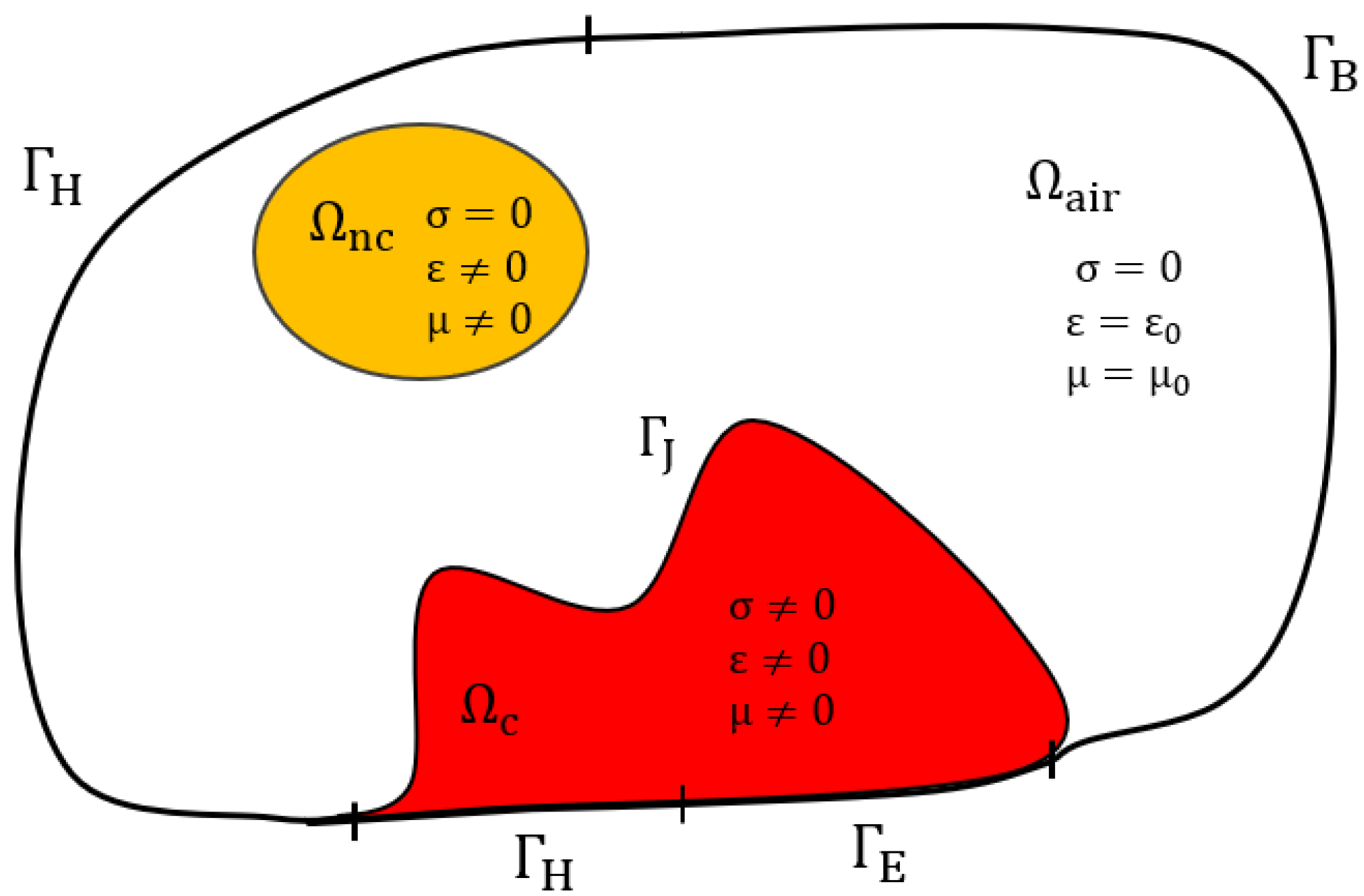
The aim of our work is to investigate the limits of the above-mentioned quasistatic models in the general case, particularly for the computational domain, including both conductive and non-conductive domains, which has not been well addressed in the literature. We are interested in the frequency domain due to the impedances’ computation.
To achieve this objective, in this work, we first validated the Darwin model with an industrial example by comparing our numerical results and measurement results. To the best of the author’s knowledge, the comparison of the Darwin model with real measurement results has not been reported in the literature. Secondly, with an academic example, we compared all the quasistatic models in the frequency domain, by regarding different numerical aspects, namely, the current density, the electric field, the magnetic field, and the impedance.
The paper is organized as follows: the full-wave Maxwell system is briefly introduced in
Section 2. In
Section 3, the EQS, MQS, and Darwin models are presented. In
Section 4, two different examples, an industrial application and an academic electromagnetic device are provided for the numerical parts. Finally, the conclusion is given in
Section 5.
3. Different Quasistatic Models
In low frequencies, by neglecting the radiation effects, several approximated models can be derived from Maxwell’s equations based on the known Galilean limits [
14,
15]. There are three main different approaches: one is electric, called the EQS model, one is magnetic, called the MQS model, and one is electric and magnetic at the same time, called the Darwin model.
Let us denote v the velocity of the system with modulus , where L and T denote the units of space and time, respectively. We compare this with the light celerity in the continuous medium . In the literature, the condition is used to classify the quasistatic models, but this condition is not sufficient to distinguish between the EQS, MQS, and Darwin models.
In vacuum, if we consider this in the one-dimensional case, Equation (
1) directly implies
then, we can obtain
where
is the order of magnitude of
, (
represents the electromagnetic fields
or
). The notation
means that the quantities
x and
y have the same order of magnitude.
Similarly, from Equation (2), we can obtain
3.1. EQS Model
Suppose that assumption (
14) holds and
, the EQS model has to be adopted. This means that the term
defined in the Maxwell–Faraday’s law, as given in Equation (
1), becomes negligible, which implies that the induced current density is neglected. Applying the divergence operator to Equation (2), the charge conservation law in the frequency domain reads
Then, an electric scalar potential (ESP)
can be introduced, such as
with
as a constant. By combining the expression of
with (10), (11), and (
15), the potential formulation for the EQS model reads
To apply a voltage excitation on the terminals of the winding corresponding to the sub-domain , Dirichlet boundary conditions are imposed on . By applying the finite element (FE) method, the ESP is discretized using the nodal elements, which introduces a symmetric matrix system.
3.2. MQS Model
Suppose that assumption (
13) holds and
: the MQS model has to be adopted. This means that the term
defined in the Maxwell–Ampere’s law, as given in Equation (2), becomes negligible, which implies that the displacement current is neglected in the dielectrics. The MQS model is derived as follows
From (21), the magnetic vector potential (MVP)
can be introduced, such as
and the ESP
is only defined in the conductive sub-domain, as follows
Combining the expressions of
and
with (
9), (10), and (20), the
-
potential formulation for the MQS model reads
where
is the magnetic reluctivity (the inverse of the magnetic permeability
). Applying the FE method, the MVP
is discretized with the edge elements and the ESP
with the nodal elements, which introduce a symmetric matrix. It should be mentioned here that the resultant matrix is not gauged. The uniqueness of
can be ensured by adding the Coulomb gauge [
15] or the tree gauge [
16].
3.3. Darwin Model
By the Helmholtz decomposition, the electric field
can be split into two parts: an irrotational part
, which is curl free, and a solenoidal part
, which is divergence free [
17]
We rewrite the Maxwell equations using this decomposition in vacuum
Based on the above system and on the Galilean limits, there are two orderings [
18]
This mixed ordering eliminates radiation effects; then, the Darwin model reads
It can be observed that the Darwin model neglects the rotational part of the displacement current densities with
. From (
28),
can be represented by the gradient of the scalar electric
while
can be represented by the time derivative of the magnetic vector
Combining (
38) with (
9), (10), and (35), the
-
potential formulation for the Darwin model [
9] reads
It should be mentioned here that the ESP is defined in the whole domain and the boundary conditions are the same as for the MQS model.
However, differing from the case of MQS model, the resultant FE matrix is non-symmetric. Moreover, the matrix is ill-conditioned due to the high contrast in the magnitudes of material coefficients [
9], which makes the convergence rate very slow, with the iterative solvers. A Coulomb type gauge as
can be imposed to make the matrix system symmetric, and direct solvers are used to ensure the stability of the convergence [
11]. However, it is difficult to use the direct solvers for industrial applications due to the memory limitations, since the number of degrees of freedom (DoF) is relatively large in practice. Thus, in this work, the iterative solver is always preferred. Without the preconditioner, the convergence with iterative solvers is sometimes prone to errors, and causes a delay in convergence and failure to find an acceptable solution.
In our study, the biconjugate gradient stabilized (BiCGSTAB) solver [
19] is implemented with a Split–Jacobi preconditioner to solve the unsymmetric system
given in (
39). The deriving preconditioner splits the Jacobi preconditioner
(
is the diagonal of
) as
, where
. Then, the final system to solve is given as follows
4. Numerical Validation
All the formulations presented in
Section 3 were implemented in our academic software
code_Carmel (
https://code-carmel.univ-lille.fr/, accessed on 20 November 2021), which provided the numerical simulation results. In the following, two different examples were carried out. For the first example, we validated the simulation results obtained with he Darwin model by considering an industrial transformer. The experimental measurement data, in a common mode test, were provided until 100 MHz. However, based on the measurement results, it should be mentioned here that the Darwin model is not valid when the frequency is superior to 10 MHz, since the radiation effects become non-neglected. As the frequency increases, to handle the skin effect in the periphery of the windings, more elements are needed in the mesh, which introduces a scientific challenge at the numerical aspect. For our computation, the total DoFs reached 40 million elements. The second one, which represents an inductance example, is studied to investigate the influence of the frequency on the electromagnetic field distributions and compare the impedance curves computed by each model, namely, EQS, MQS, and Darwin models.
4.1. Industrial Application
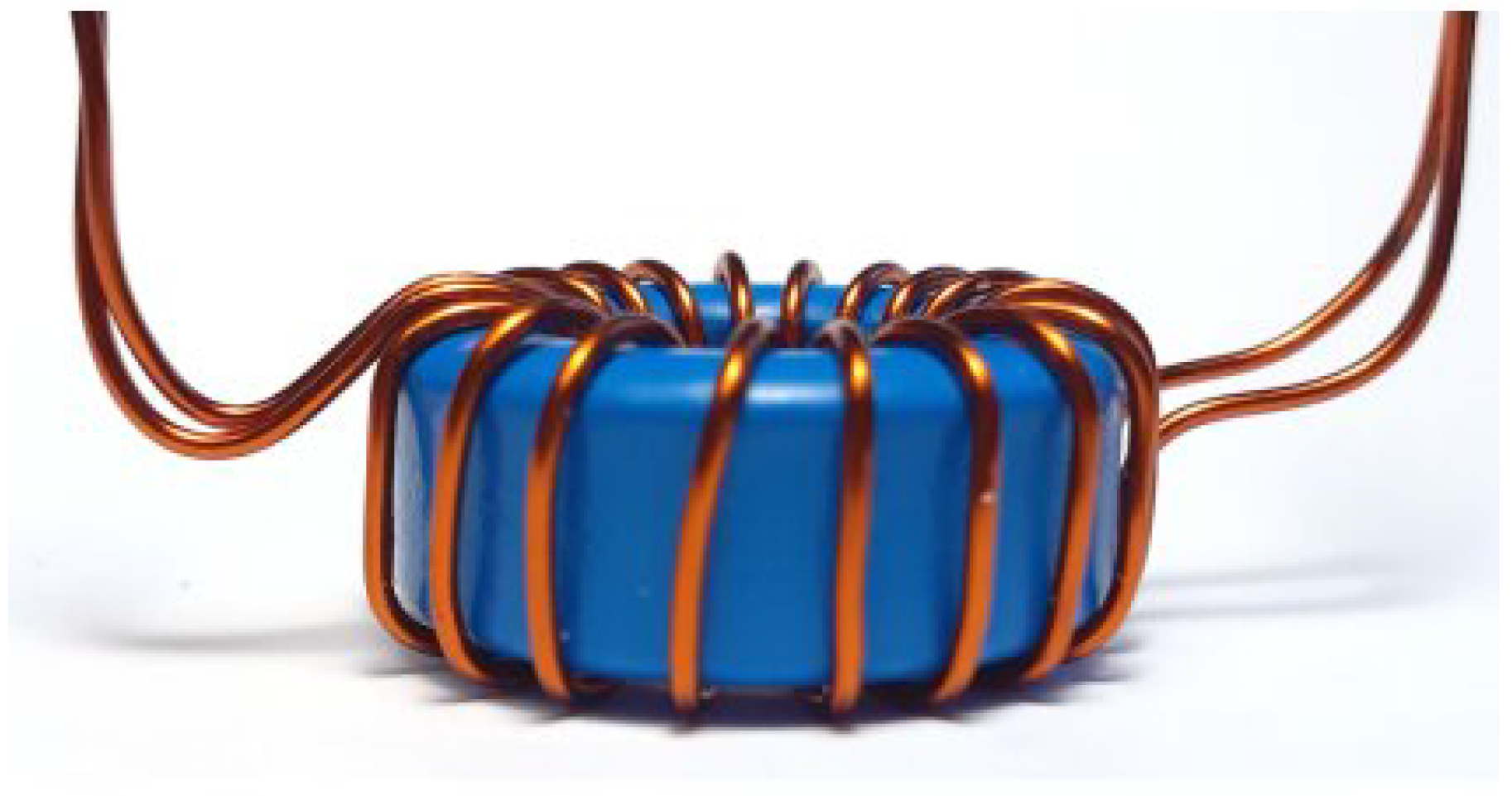
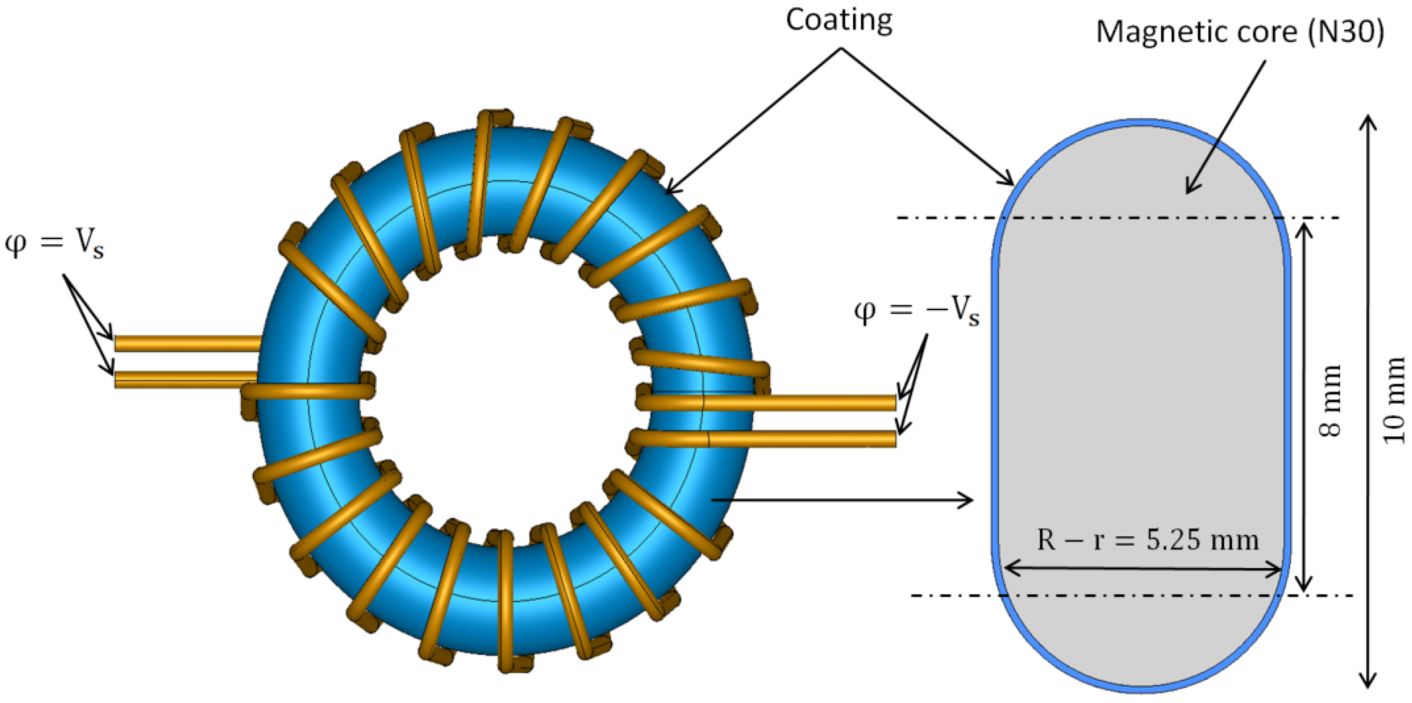
For the first example, the geometry consists of two windings wound in the same direction around a toroidal core, as shown in
Figure 2,
Figure 3 and
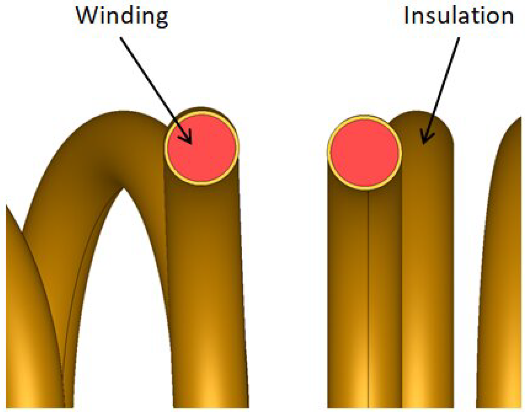
Figure 4. The conductor used for the windings was made of copper, presented in red in
Figure 4: it was circular in shape and each conductor was composed of 10 turns with a section of
. The enamel component covered the winding with a thickness of
. The toroid used for this experiment was a TDK-Epcos toroid reference B64290L0618X830 (
https://product.tdk.com/en/search/ferrite/ferrite/ferrite-core/info?part_no=B64290L0618X830, accessed on 20 November 2021), of material N30 presented in gray in
Figure 3, where the material in blue is the embedding with a thickness of
mm. The conductivity of the conductor is equal to
, while the enamel was emphasized so that the relative permittivity was set as
.
4.1.1. Computational Configurations
An electric potential difference
was imposed between the terminals of the conductor of the windings marked in red, as shown in
Figure 4. A single-phase common mode test was considered in this example, which means that
was imposed on one terminal of the conductor and
on the other, as shown in
Figure 3. The frequency interval was [0:10
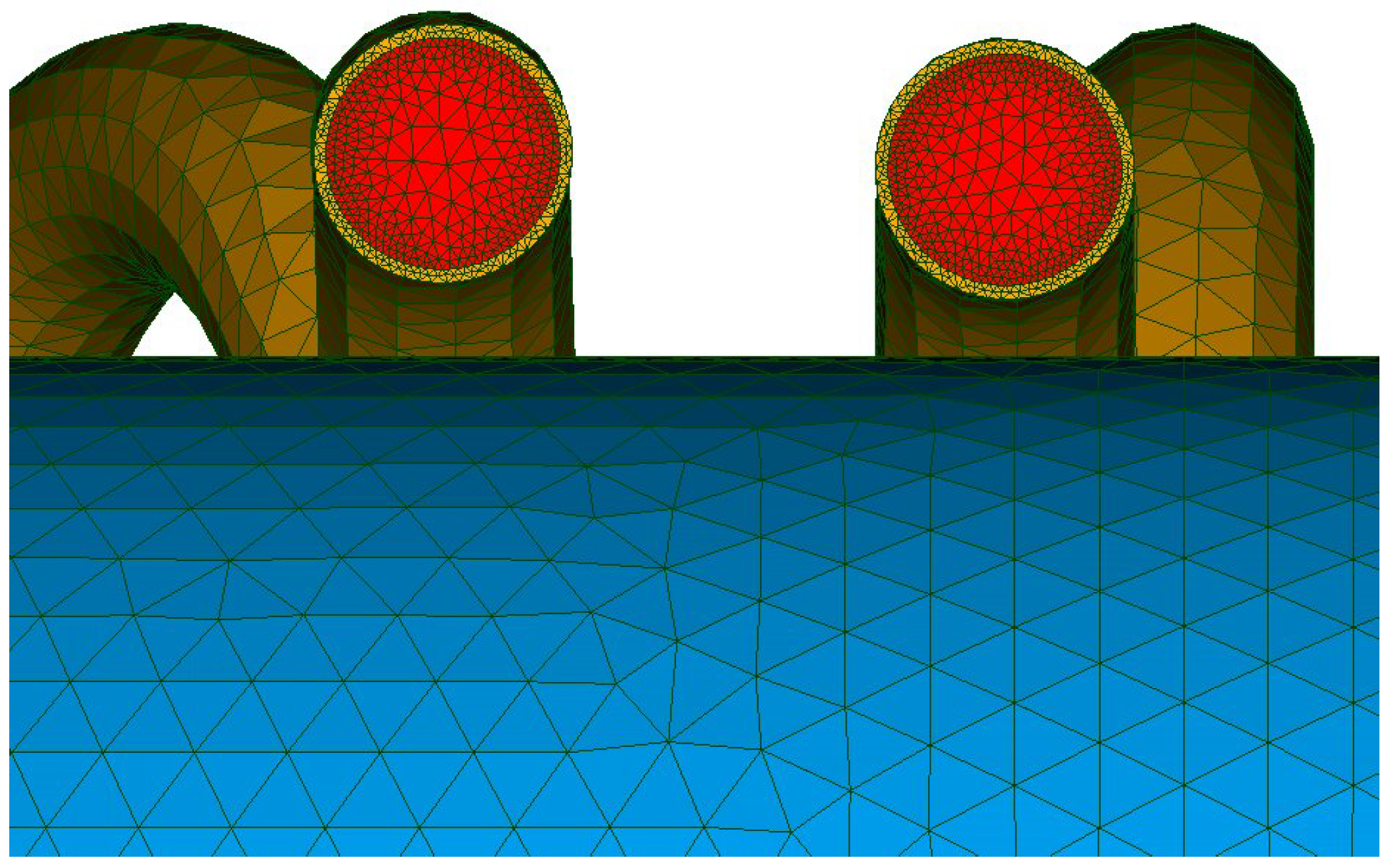
] Hz. To handle the skin effect, the considered mesh was well-refined and suitable for all frequencies up to 1 MHz, which featured 29,832,477 tetrahedrons including 5,257,323 nodes and 35,093,396 edges. For each frequency, the computing time using the Darwin model took about 9 days for 40,338,477 DoFs using the BiCGSTAB solver. Notably, for a system with a large DoFs, the BiCGSTAB is always preferred to direct solvers because the latter may fail due to the relative need for memory, which is much larger than that required for the iterative solvers. The mesh of the winding and the toroidal core are presented in
Figure 5.
4.1.2. Electric Potential and Electric Field
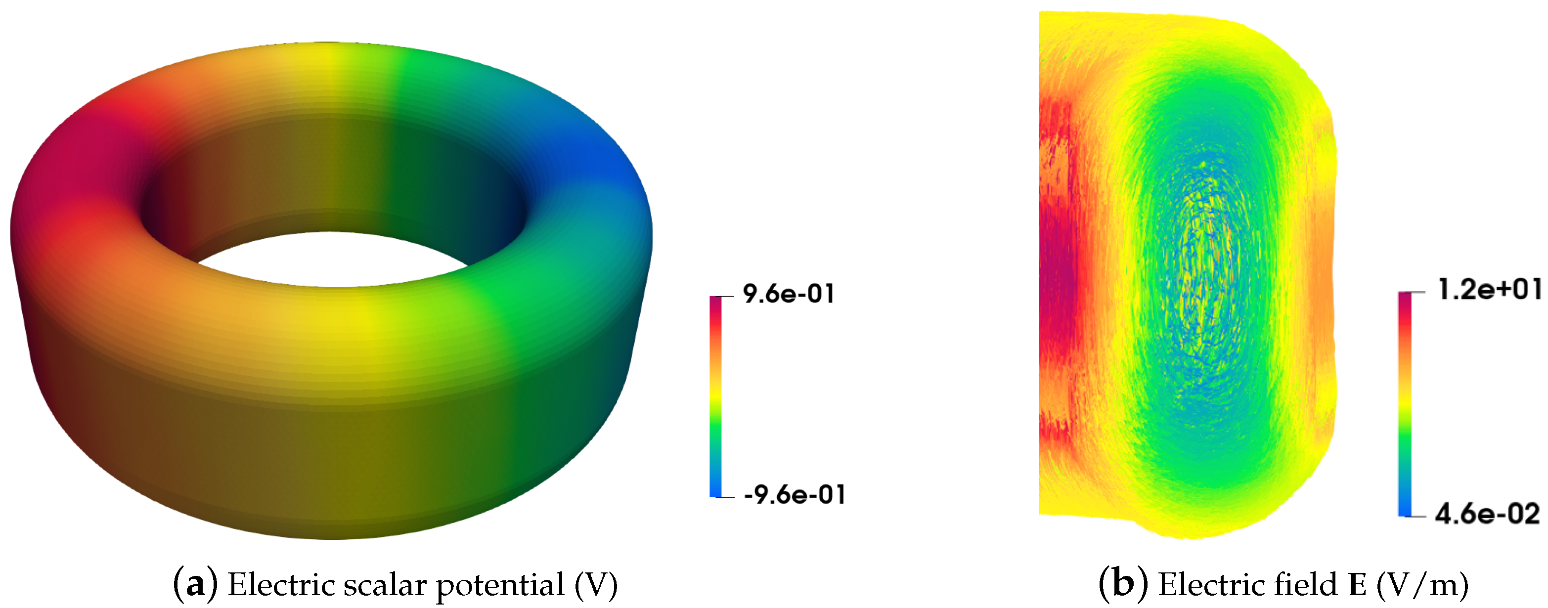
The electric scalar potential along the magnetic core is presented in
Figure 6a, which shows a decreasing linear variation in its magnitude. In addition, the electric field distribution in a sectional view is also given in the magnetic core, as shown in
Figure 6b. It can be observed that the electric field is located in the periphery of the core due to the skin effect that occurs, and reaches a maximum value of
.
4.1.3. Conduction and Displacement Current Densities
When the frequency increases, the total current is divided into two parts: the conduction current in the conductive domains and the displacement current located in the non-conductive domains. This means that the displacement current intervenes in the modeling of the electric field, in addition to the eddy current.
On one hand, the conduction current density is presented in
Figure 7a in the windings for a frequency of 500 kHz. High values are observed inside each of the two conductors. Due to the skin effect, the current is concentrated in the small layer at the boundary of the conductor. Moreover, the peaks were higher near the middle section, mainly due to the magnetic coupling known as the proximity effect.
On the other hand, as shown in
Figure 7b, the displacement current density is presented in a sectional view of the magnetic core for a frequency of 500 kHz. The distribution shows that the significant quantity of current is located between the turns, as the magnitude tends to be zero in the contact area with the windings, due to the capacitive effects.
4.1.4. Measurement and Simulation Comparison
In
Figure 8, the evolution of the impedance as a function of the frequency obtained from Darwin model, as well as the phase, are presented.
First, the impedance corresponds to the DC resistance of the winding when the frequency tends towards zero. Indeed, we have .
Second, for kHz, the results obtained with the Darwin are in good agreement with the measurement results, which present the resistive–inductive phenomena, such as the MQS regime.
Third, the resonant frequency is around 1 MHz; the simulation result of the Darwin model shows a close result at the chosen point of the frequency (7th point), just before the resonant frequency. It can be found that this point is no longer in the MQS regime, since the impedance at this point is not linear to the previous points. A similar behavior can be observed for the phase as a function of the frequency.
4.2. Modeling of the Academic Electromagnetic Device
For the second example, we are interested in determining the operating frequency domain of different models. Some validation work was carried out with the static or/and MQS and EQS models, as shown in [
20,
21]. The objective was to study the influence of the frequency on the distribution of electromagnetics fields, as well as on the impedance obtained using the models mentioned in
Section 3.
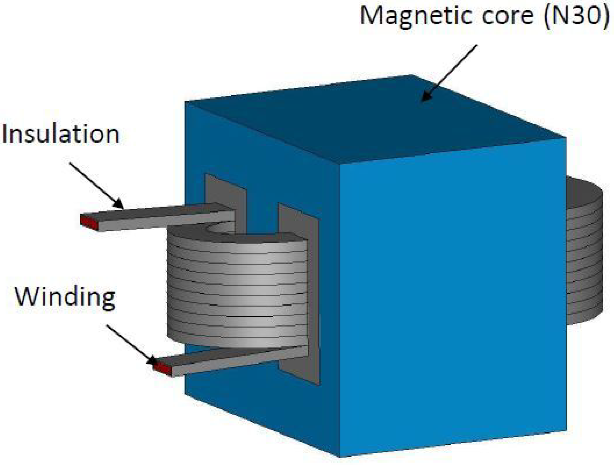
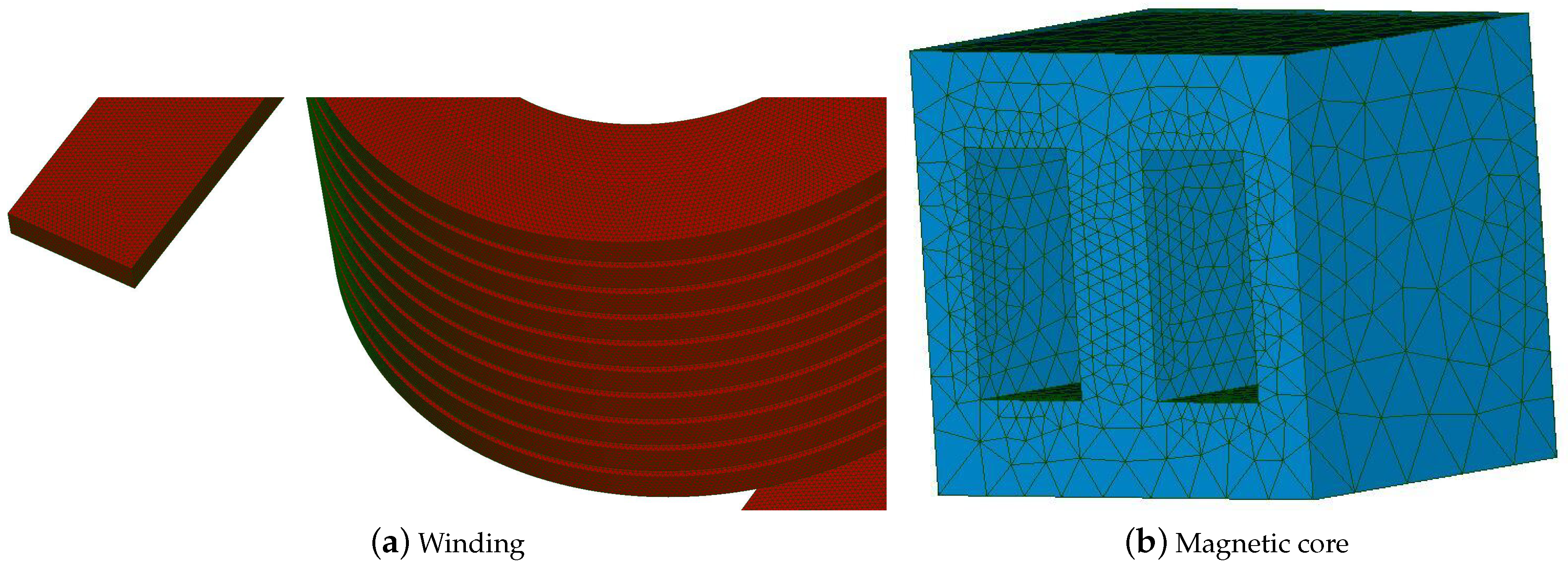
As shown in
Figure 9, the electromagnetic device composed of a winding (shown in red color) coiled around the central column of the magnetic core (shown in blue color) was considered. We have a conductor of section
which takes a rectangular shape. It is composed of 11 turns and has a length of
m. The insulation covered the winding with a thickness of
mm. The magnetic core was composed of
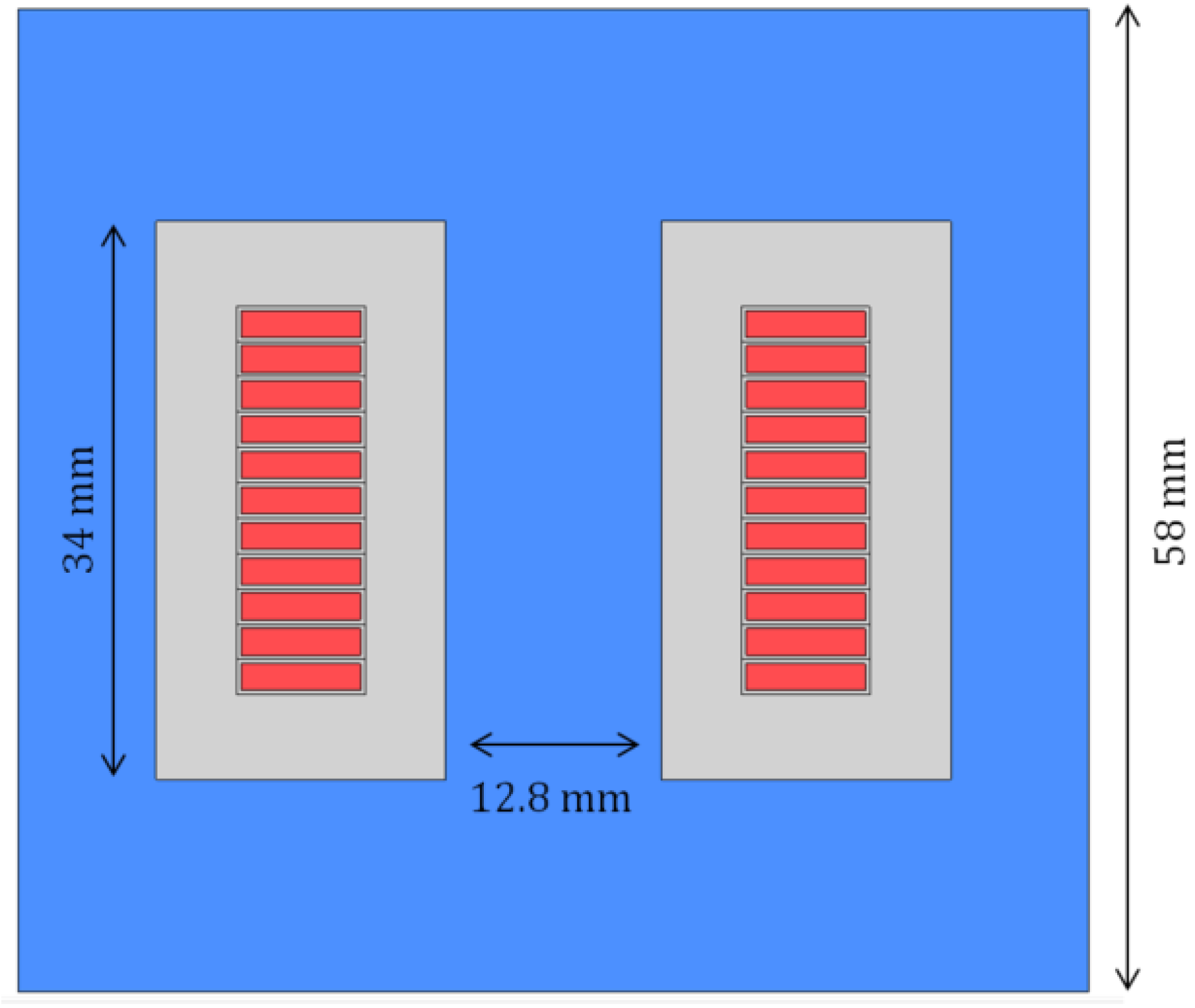
-ferrite. This inductance is shown in 2-D cutting plane in
Figure 10.
The conductivity of the copper coil is set as . The insulation covered the winding, and it is emphasized that the relative permittivity was set as when the magnetic core is composed of -ferrite, characterized by a relative permeability of 4300, an electric permittivity of 80 and an electric conductivity fixed to zero. The electric potential on the below face of the magnetic core was taken to be zero, which corresponds to connect to the ground.
4.2.1. Computational Configurations
A sinusoidal voltage was applied between the terminals of the winding marked in red, as shown in
Figure 9. The frequency interval was [0:10
] Hz. To consider the skin effects in the winding for high frequencies, the mesh used for the model featured 14,443,563 tetrahedrons, including 2,466,531 nodes and 16,911,563 edges. The mesh of the winding and the magnetic core are presented, respectively, in
Figure 11a,b. For the EQS model, the number of DoFs is 2,466,002 and the computational time for one frequency takes about two hours, while it takes about 75 hours for 19,316,839 DoFs in the MQS model. The computing time using Darwin formulation takes about 86 hours for 19,373,155 DoFs. It should be recalled here that the matrix system associated with MQS is symmetric, while this is not the case for the Darwin model. In the general case, the computational cost for the MQS model is less expensive than Darwin’s due to the ill-conditioned matrix of the Darwin model, and different preconditioners can be applied for MQS and Darwin cases. Moreover, the computational cost for the EQS model is relatively low in comparison with the two other models.
Additionally, It should be mentioned that the condition number of the matrix depends on the frequency for both MQS and Darwin models. Consequently, the number of iterations associated with the iterative solver, which is required to achieve the solution’s convergence, is not the same. For example, for
and with a fixed stopping criterion, the number of iterations associated with BiCGSTAB is 14 k using the MQS model, while it takes about 17 k for the Darwin model, as shown in
Table 1.
4.2.2. Distribution of Electric and Magnetic Fields
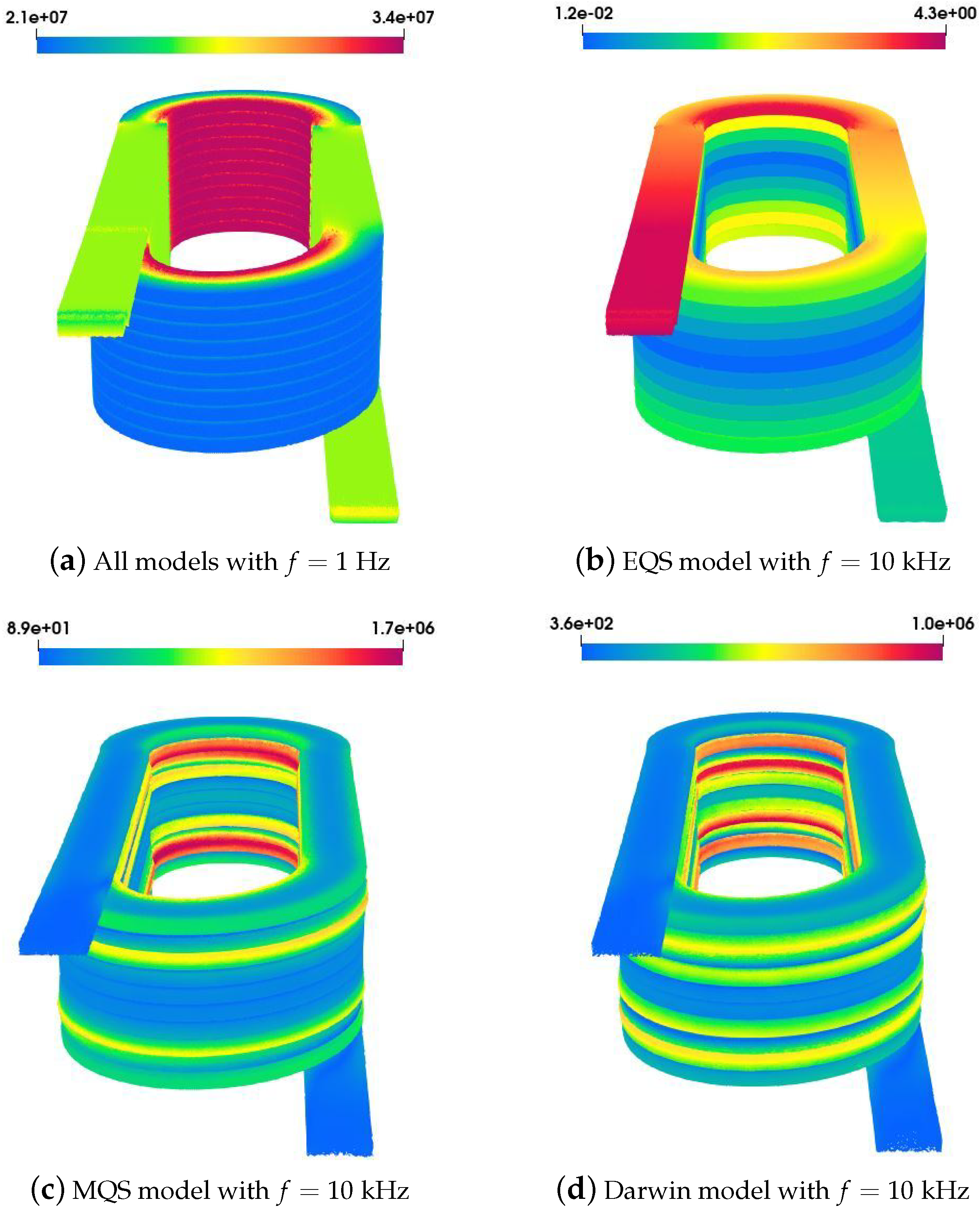
At low frequencies, when the frequency tends towards zero, the distribution of the current density in the winding obtained with all models is similar, as observed in
Figure 12a, since this is equivalent to solve an electrokinetic problem. In this case, the distribution of the current density is only influenced by the geometry of the winding. When the frequency supplying the winding increases, coupled effects may be observed. To represent these effects in the winding, the distribution of the current density
is presented in
Figure 12b–d. At
, with the EQS model, it is clear that
will never be homogeneous along the winding; the majority of currents flow through the capacitor in terms of the displacement current. On the other hand, the current density with the MQS and Darwin models is restricted to a small layer at the boundary of the winding, and starts to flow in the outskirts of the conductor, as observed by the skin effect.
Besides, due to the capacitive effects, the current density distribution obtained with the Darwin model is not the same as that of MQS. The irrotational current density is much larger in both cases, compared to the solenoidal one, such that the capacitive coupling cannot be distinguished from
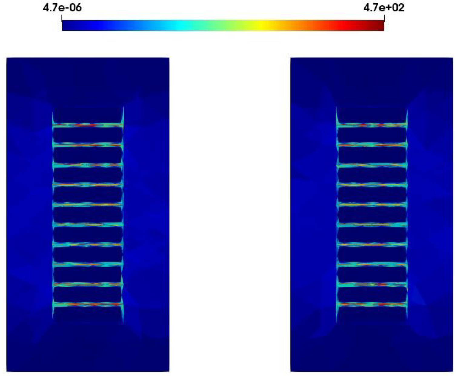
Figure 12d. Moreover, the distribution of the electric field obtained from the Darwin model is presented in
Figure 13 in a 2-D cutting plane for
. A high field strength appears in the dielectric regions, particularly between the gaps of the winding.
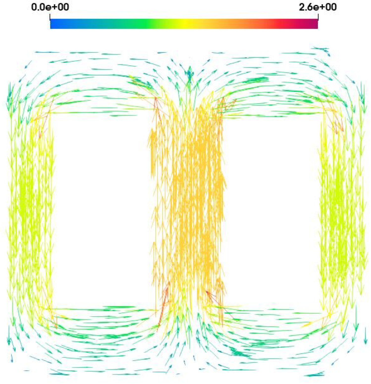
In addition, when capacitive effects are neglected for low and middle frequencies, both MQS and Darwin problems give the same distribution of the magnetic flux density. Then, when the frequency tends towards zero, the distribution of the magnetic flux density obtained from MQS and Darwin models is equivalent to solve a magnetostatic problem, as shown in
Figure 14.
4.2.3. Evolution of the Impedance Versus the Frequency
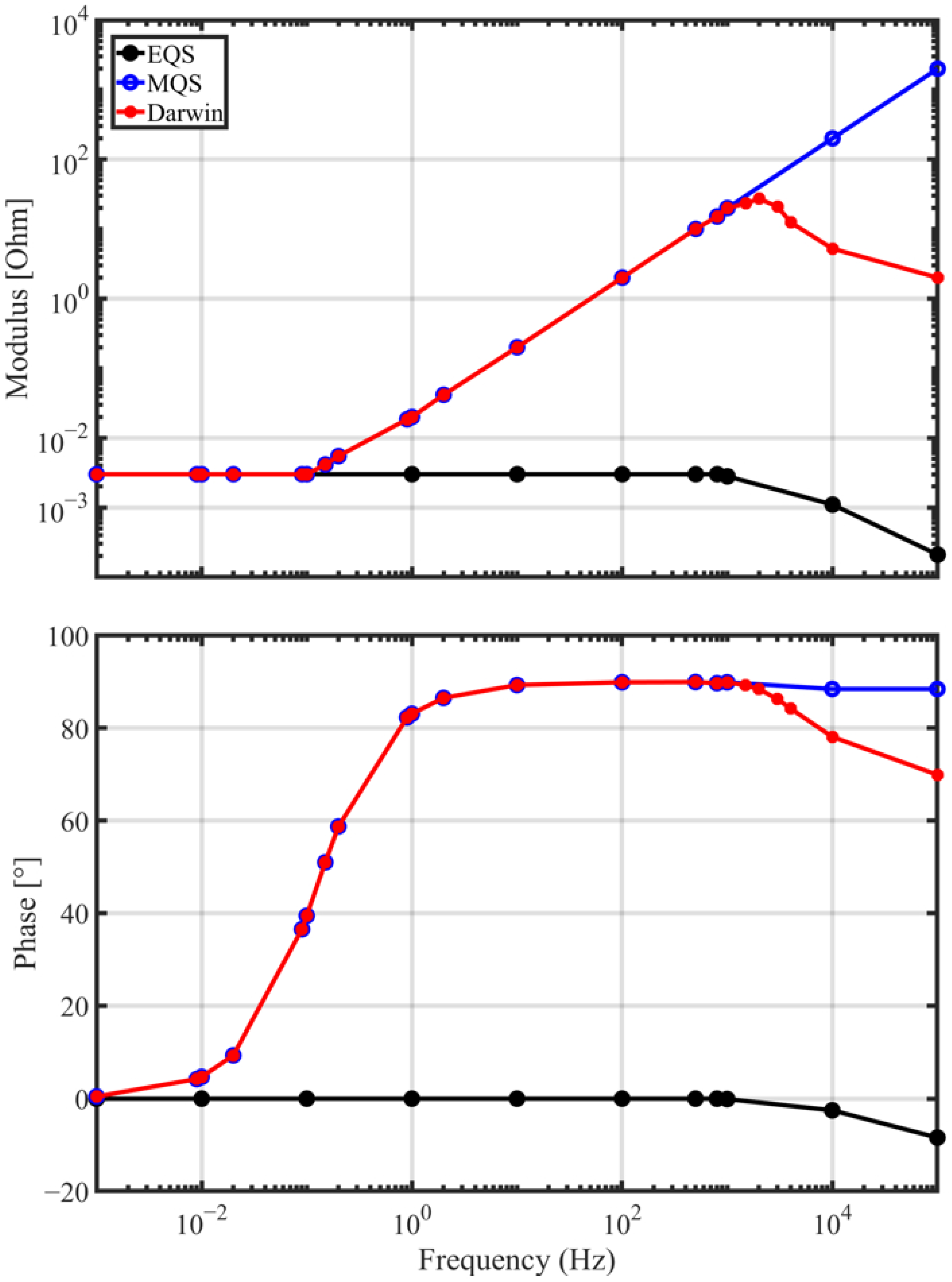
The evolution of the impedance modulus and its phase, according to the frequency obtained from EQS, MQS, and Darwin models, are presented in
Figure 15. At low frequencies, the impedance
corresponds to the DC resistance of the winding. Then, for all models, we obtain
when the frequency tends towards zero. When the frequency increases, the skin effect appears in the winding; then, the value of the resistance of the winding increases. This effect is not taken into account with the EQS model. For
:
, the MQS and Darwin models give a similar evolution of the impedance. Indeed, the capacitive effect is negligible compared with the inductive and resistive effects. For
, the influence of the the capacitive effects appears on the evolution of the impedance for both the EQS and Darwin models. A similar behavior can be observed for both models in
Figure 15.
5. Conclusions
In this work, the measurement results for an industrial example have been provided to validate the simulation results obtained with the Darwin model, which shows a good agreement in the range of intermediate frequencies, particularly around the resonant frequency. Additionally, for a complex and multi-domain application, the different quasistatic models were compared by computing their impedances, as well as the different electromagnetic fields, to investigate their limits.
At low frequencies, when the impedance exhibits a resistive behavior, the EQS model is sufficient. Moreover, when the inductive effects are non-neglected, the MQS and Darwin models can be invoked, but the MQS model is preferred, since its computational cost is lower than the Darwin model. However, in the intermediate frequencies, particularly around the resonant frequency, the Darwin model should be adopted, since the MQS model cannot handle the coupled capacitive-inductive effects.
Furthermore, the EQS model can be used as an indicator to learn the frequency at which the capacitive effects become significant, where the Darwin model should be applied.


 ,
, 


