Multivariable Adaptive Super-Twisting Guidance Law Based on Barrier Function

Abstract

For tactical missiles, sliding mode control and super-twisting algorithms have been widely studied in the area of guidance law design. However, these methods require the information of the target accelerations and the target acceleration derivatives, which is always unknown in practice. In addition, guidance laws utilizing these tools always have chattering phenomena and large acceleration commands. To solve these problems, this article introduces a barrier function based super twisting controller and expands the controller to a multivariable adaptive form. Consequently, a multivariable adaptive super-twisting guidance law based on barrier function is proposed. Moreover, the stability of the guidance law is analyzed, and the effectiveness and the robustness are demonstrated by three simulation examples. Compared with previous guidance laws using sliding mode control or super-twisting algorithm, the one proposed in this paper does not require the information of target accelerations, nor target acceleration derivatives; it has smaller super-twisting gains so that has smaller acceleration commands; it can increase and decrease the gains to follow the target accelerations and maintain the sliding mode, and it does not chatter.

1. Introduction

Precision guidance has always been a key technology in missile control field with the development of flight vehicles. Due to the convenience of implementation and the accuracy of interception, the proportional navigation guidance (PNG) law and its variants [1,2,3,4] have been widely used in various engineering practices. PNG methods are designed to keep the line-of-sight (LOS) angular rate converge to zero to intercept targets. However, in practice, the maneuvers of the target, desired constraints and the disturbances of measurement may lead to poor results of PNG.

Hence, a series of modern guidance laws based on advanced control theory have been proposed to address the problems. References [5,6] introduced optimal control theory into waypoint-following guidance problems and calculated the guidance law by solving optimal control problems. On the basis of H-infinite theory, reference [7,8] proposed robust guidance laws by regarding unpredictable target maneuvers as bounded unknowns. Reference [9] disposed of the constraints and the performance index by using the convex optimization method to obtain guidance gains. Utilizing model predictive control, reference [10] designed a suboptimal terminal angle constrained guidance law.

At the same time, due to the inherent properties of strong robustness against external disturbances and uncertainties of systematic parameters, the sliding mode control (SMC) [11,12,13,14] theory was applied to guidance law design, especially in the scenarios with constraints. To obtain a global stable guidance law, the LOS angles are utilized to construct the sliding manifold so that the sliding manifold could converge to zero or the neighborhood of zero. In [15], a three-dimensional adaptive finite-time guidance law that can accelerate the convergent rate was presented. After that, reference [16] presented an analytical solution with input saturation for [15]. Reference [17] proposed an adaptive reentry guidance law for the hypersonic vehicle with a specified impact angle. By employing a second-order sling mode observer, reference [18] proposed a nonsingular terminal sliding mode guidance law with autopilot lag consideration. The integral sliding mode guidance law presented in [19] addressed the problem of steady-state error of the traditional SMC. Reference [20] implemented an optimization design by using the neural network, which improved the fuzzy variable structure of the sliding mode. Moreover, ref. [21] designed an adaptive anti-saturation integral sliding mode guidance law by introducing an auxiliary system to solve the problem of input saturation. However, to keep the sliding surface on zero or in the neighborhood of zero, the control commands of sliding mode controllers are always discontinuous, sometimes even chatter distinctly. The phenomenon of chattering may lead to undesirable implementation of the actuators [22].

To eliminate the chattering of sliding mode guidance law, the super-twisting algorithm (STA) [23] controller became popular. Denoting the target accelerations as the disturbances, the STA controller can reach the sliding mode by designing the gains of the super-twisting controller to counteract the disturbances. The dynamical adaptation gains are expected to be as small as possible meanwhile sufficient to offset the disturbances. Some super-twisting methods are based on the usage of the filtered value of the equivalent control as an estimation of the disturbance [24,25,26]. Moreover, some are based on increasing gains [27,28]. Additionally, super-twisting methods are applied in the area of guidance law design. Reference [29] designed an STA-like guidance law considering actuator faults based on the equivalent control value. References [30,31] designed adaptive STA guidance laws which could be convergent in finite time based on the increasing gains. Introducing a faster convergence error form, ref. [32] proposed a modified adaptive STA guidance law considering seeker delays. However, these STA controllers have some disadvantages: the methods in [24,25,26,29,32] require the upper bounds of disturbances derivatives to select the filter constants; and the gains of methods in [27,28,30,31] keep increasing throughout the progress, and cannot follow disturbances when they are decreasing, which may lead to large output, or even instability.

In order to overcome these drawbacks, references [33,34,35] proposed barrier function-based adaptive super-twisting controllers. The algorithm based on barrier function can drive the output variable in a predefined neighborhood of zero and then keep on it. However, the missile guidance system with terminal angle constraint is a multivariable problem, the existing barrier function-based method cannot be applied directly.

Inspired by the above works, this study presents a multivariable barrier function-based super-twisting controller and applied the algorithm to guidance law design with impact angle consideration for a maneuvering target. Compared with other sliding mode control or super-twisting guidance laws, the distinguishing properties of the guidance law suggested in this paper can be concluded as follows:

• The guidance law does not require the information of disturbance derivatives, nor utilize a filter to obtain the value of equivalent control;
• The super-twisting gains of the guidance law are small but sufficient to counteract the disturbances, and consequently, the output variable (acceleration command) is small but adequate to achieve performance goals;
• The guidance law can converge to a predefined neighborhood of zero and maintain the sliding mode, whether the disturbances increase or decrease;
• The acceleration commands have no chatterings.

The rest of the paper is organized as follows: Section 2 presents the kinematics of missile-target engagement and preliminaries; Section 3 designs a multivariable adaptive super-twisting guidance law based on barrier function and analyzes the stability, and Section 4 gives three simulation examples to demonstrate the effectiveness and robustness of the proposed guidance law.

2. Problem Statement

In order to facilitate the later design of the barrier function-based super-twisting guidance law, the missile-target engagement kinematics and some preliminaries are introduced in this section.

2.1. Kinematics of Missile-Target Engagement

Figure 1 demonstrates the three-dimensional pursuit geometry relationship between missile and target, where ${\left[\begin{array}{ccc}{e}_r& e_{{}_{\theta }}& e_{\varphi }\end{array}\right]}^T$ is a unit vector aligned with the three axes of the LOS coordinate system. Denoted $(X,Y,Z)$ and $(r,\theta ,\varphi )$ as the inertial coordinate system and the line-of-sight (LOS) coordinate system, respectively, where $r$, $\theta$ and $\varphi$ represent the relative distance between the point masses of missile and target, the azimuth and elevation angles of the LOS, respectively. Then, the missile-target engagement kinematics can be described by the LOS coordinate system with the origin at the mass center of the missile, and the relative velocity in LOS coordinate system $V$ is given by:

$$V={\left[\begin{array}{ccc}\dot{r}& r\dot{\theta }\cos \varphi & r\dot{\varphi }\end{array}\right]}^T$$

(1)

where $\dot{\theta }$ and $\dot{\varphi }$ represent the azimuth and elevation angular rates of LOS, respectively. The relative velocity satisfies the following vector differential form:

$$\frac{d\mathit{V}}{dt}=\frac{\delta \mathit{V}}{\delta t}+\omega \times \mathit{V}=a_T-a_M$$

(2)

where $d\mathit{V}/dt$ and $\delta \mathit{V}/\delta t$ denote the absolute derivative of $\mathit{V}$ in an inertial coordinate system, and the relative derivative of $\mathit{V}$ in an LOS coordinate system, respectively; $a_T$ and $a_M$ denote the accelerations of the target and missile, respectively; $\omega$ denotes the relative rotation angular velocity of LOS coordinate system in inertial coordinate, which satisfies the following expression:

$$\omega ={\left[\begin{array}{ccc}\dot{\theta }\sin \varphi & -\dot{\varphi }& \dot{\theta }\cos \varphi \end{array}\right]}^T$$

(3)

Substituting Equations (1) and (3) into Equation (2), the three-dimension missile-target engagement kinematic equations can be formulated as:

$$\{\begin{array}{l}\ddot{r}={\dot{\theta }}^2{\cos }^2\varphi r+{\dot{\varphi }}^{2}r+a_{Tr}-a_{Mr}\hfill \\ \ddot{\theta }=2\dot{\varphi }\dot{\theta }\tan \varphi -\frac{2\dot{r}\dot{\theta }}{r}+\frac{a_{T\theta }}{r\cos \varphi }-\frac{a_{M\theta }}{r\cos \varphi }\hfill \\ \ddot{\varphi }=-{\dot{\theta }}^2\sin \varphi \cos \varphi -\frac{2\dot{r}\dot{\varphi }}{r}+\frac{a_{T\varphi }}{r}-\frac{a_{M\varphi }}{r}\hfill \end{array}$$

(4)

where ${\left[\begin{array}{ccc}{a}_{Tr}& a_{T\theta }& a_{T\varphi }\end{array}\right]}^T$ and ${\left[\begin{array}{ccc}{a}_{Mr}& a_{M\theta }& a_{M\varphi }\end{array}\right]}^T$ are components of target and missile accelerations along the LOS coordinate axes, respectively.

Remark 1.

From Equation (4), one can easily conclude that$r=0$, and$\varphi =\pm \pi /2$are singular points of the control system. However, in real practice, the distance between point masses of missile and target tends to be zero but not zero due to their realistic physical structure. Thus, the scenario$r=0$does not occur throughout the guidance process. As for regular points$\varphi =\pm \pi /2$, the study work in [14] in the planar homing engagement phase proved that these points are not the stable equilibrium cases. Hence, the guidance process just crosses them without staying.

In consideration of the constraint of desired LOS terminal angles ${\theta }_d$ and ${\varphi }_d$, denote ${\mathit{x}}_1={\left[\begin{array}{cc}{x}_{1\theta }& x_{1\varphi }\end{array}\right]}^T={\left[\begin{array}{cc}\theta -{\theta }_d& \varphi -{\varphi }_d\end{array}\right]}^T$ and ${\mathit{x}}_2={\dot{x}}_1={\left[\begin{array}{cc}{x}_{2\theta }& x_{2\varphi }\end{array}\right]}^T={\left[\begin{array}{cc}\dot{\theta }& \dot{\varphi }\end{array}\right]}^T$ as the control variables, and substitute into Equation (4) yields:

$$\begin{array}{l}{\dot{x}}_1={\mathit{x}}_2\\ {\dot{x}}_2=\mathit{F}(\mathit{x})+Bu+\Delta \end{array}$$

(5)

where:

$$\begin{gathered} F=\left[\begin{array}{c}2x_{2\theta }{x}_{2\varphi }\tan \varphi -\frac{2\dot{r}{x}_{2\theta }}{r}\\ -x_{2\theta }^2\sin \varphi \cos \varphi -\frac{2\dot{r}{x}_{2\varphi }}{r}\end{array}\right], B=\left[\begin{array}{cc}-\frac{1}{r\cos \varphi }& 0\\ 0& -\frac{1}{r}\end{array}\right] \\ u=a_M={\left[\begin{array}{cc}{a}_{M\theta }& a_{M\varphi }\end{array}\right]}^T,\mathsf{\Delta }=\left[\begin{array}{cc}{\mathsf{\Delta }}_1& {\mathsf{\Delta }}_2\end{array}\right]={\left[\begin{array}{cc}\frac{a_{T\theta }}{r\cos \varphi }& \frac{a_{T\varphi }}{r}\end{array}\right]}^T \end{gathered}$$

(6)

2.2. Preliminaries

Definition 1.

Consider there exists a fixed and known positive constant$\epsilon$. For any given positive number$b$, a barrier function can be defined as a continuous function$L_b\left(x\right)$in the interval$x\in (-\epsilon ,\epsilon )$, which satisfies:

• ${\lim }_{\left|x\right|\to \epsilon }{L}_b(x)=+\infty$;
• $\min (L_b(x))=L_b(0)=b$;
• $L_b(x)$is strictly decreasing and increasing in$x\in (-\epsilon ,0]$and$x\in [0,\epsilon )$, respectively.
• Figure 2shows the barrier function of this paper, which is given by:

  $$L_b(x)=\frac{\sqrt{\epsilon }b}{{\left(\epsilon -\left|x\right|\right)}^{1/2}},x\in (-\epsilon ,\epsilon )$$

  (7)

Notation 1.

For any given vector$x={\left[\begin{array}{cccc}{x}_1& x_2& \cdots & x_n\end{array}\right]}^T$, denote its absolute value as$\left|x\right|={\left[\begin{array}{cccc}\left|x_1\right|& \left|x_2\right|& \cdots & \left|x_n\right|\end{array}\right]}^T$, its time derivative as$\dot{x}={\left[\begin{array}{cccc}{\dot{x}}_1& {\dot{x}}_2& \cdots & {\dot{x}}_n\end{array}\right]}^T$, its sign function as$sign(x)={\left[sign(\begin{array}{cccc}{x}_1)& sign(x_2)& \cdots & sign(x_n)\end{array}\right]}^T$, its second power as$x^2={\left[\begin{array}{cccc}{x}_1^2& x_2^2& \cdots & x_n^2\end{array}\right]}^T$, and its 2-norm as$\Vert x\Vert =\sqrt{x^{T}x}$. For any positive definite matrix$P$, denote${\lambda }_{\min }(P)$and${\lambda }_{\max }(P)$represent the minimum and maximum eigenvalues of$P$, respectively, and satisfyingfollowing inequation:${\lambda }_{\min }(P){\Vert x\Vert }^2\le x^{T}Px\le {\lambda }_{\max }(P){\Vert x\Vert }^2$. In addition, denote operation symbol “$\circ$” as Hadamard product symbol.

Assumption 1.

The total missile velocity$V_m$and target velocity$V_t$are constant, and$V_m>V_t$.

Assumption 2.

The missile flight control dynamics are fast enough such that their effects can be neglected.

3. Barrier Function-Based Multivariable Super-Twisting Guidance Law Design

In this section, a novel multivariable adaptive super-twisting controller based on barrier function is proposed. Then, following a nonsingular sliding mode surface, a novel guidance law based on the proposed controller with terminal angle constraint is formulated. Finally, the stabilization of the guidance law is proved based on Lyapunov theory.

3.1. Design of Adaptive Multivariable Super-Twisting Controller Based on Barrier Function

In consideration of a first-order system with the following form:

$$\dot{s}(t)=u(t)+\delta (t)$$

(8)

where $s(t)$ is the output variable; $u(t)$ is the super-twisting controller; and $\delta (t)$ is Lipschitz disturbance such that:

$$\left|\dot{\delta }(t)\right|\le M$$

(9)

where $M$ is the upper bound of $\left|\dot{\delta }(t)\right|$, which is always unknown in practice.

The main goal of the super-twisting controller design is to counteract the Lipschitz disturbance $\delta (t)$ and drive both $s(t)$ and $\dot{s}(t)$ to zero. The standard super-twisting controller for system (8) can be described as [23]:

$$\{\begin{array}{l}u(t)=-a_1{\left|s\right|}^{1/2}sign(s)+y(t)\hfill \\ \dot{y}(t)=-a_{2}sign(s)\hfill \end{array}$$

(10)

where $a_1$ and $a_2$ are designed gains, which satisfy $a_1=1.5\sqrt{M}$ and $a_2=1.1M$, respectively.

By introducing a twisting state variable $y(t)$, which converges to a neighborhood of zero in finite time, the controller (10) can meet the main goal. However, there are two distinct flaws in the standard super-twisting controller:

• The design of the controller gains $a_1$ and $a_2$ requires the information of M;
• The value and convergence speed of $y(t)$ relies on the designed gains $a_1$ and $a_2$.

In order to address these problems, an adaptive super twisting controller based on barrier function is proposed in [35], which is given by:

$$\{\begin{array}{l}u(t)=-L(t,s){\left|s\right|}^{1/2}sign(s)+y(t)\hfill \\ \dot{y}(t)=-L^2(t,s)sign(s)\hfill \end{array}$$

(11)

where the adaptive gain $L(t,s)$ is formulated as:

$$L(t,s)=\{\begin{array}{ll}\overline{L}(t),\hfill & 0\le t<\overline{t}(s_0)\hfill \\ L_b(s),\hfill & t\ge \overline{t}(s_0)\hfill \end{array}$$

(12)

where $s_0=s(0)$; $\overline{t}(s_0)$ is the first time for which $s(t)<\epsilon /2$; $L_b(s)$ has the same form as (7); and $\overline{L}(t)$ is given by:

$$\overline{L}(t)=l_0+l_{1}t$$

(13)

where $l_0$ and $l_1$ are designed positive constants.

Reference [35] has proved that there exists a finite time $\overline{t}(s_0)$, and after that, the barrier function gain $L_b(s)$ can drive $s(t)$ to a small neighborhood of zero. However, the super-twisting controller (10) can not be utilized directly for the multivariable system, such as:

$$\dot{s}(t)=u(t)+\delta (t)$$

(14)

Therefore, a multivariable adaptive super-twisting controller with the barrier function gain (12) is proposed in this paper, which can be expressed as:

$$\{\begin{array}{l}u(t)=-L(t,s)\circ \frac{s}{{\Vert s\Vert }^{1/2}}+y(t)\hfill \\ \dot{y}(t)=-L^2(t,s)\circ \frac{s}{\Vert s\Vert }\hfill \end{array}$$

(15)

3.2. Design of Sliding Mode Guidance Law Based on Adaptive Super-Twisting Control

In order to improve the convergence speed of the sliding variable and avoid the singularity in the meanwhile, the following sliding manifold for system (5) is taken into account, which is formulated as:

$$s=x_2+k_1{x}_1+k_{2}w(x_1)$$

(16)

where $s={\left[\begin{array}{cc}{s}_1& s_2\end{array}\right]}^T$ is the sliding manifold vector; $k_1$ and $k_2$ are designed positive constants; and term $w(x_1)={\left[\begin{array}{cc}w(x_{11})& w(x_{12})\end{array}\right]}^T$ is given by:

$$w(x_{1i})=\begin{array}{ll}\{\begin{array}{ll}{\left|x_{1i}\right|}^{k_3}sign\left(x_{1i}\right),\hfill & s_i=0or{\overline{s}}_i\ne 0,\left|x_{1i}\right|\ge \xi \hfill \\ k_4{x}_{1i}+k_5{x}_{1i}^{2}sign\left(x_{1i}\right),\hfill & {\overline{s}}_i\ne 0,\left|x_{1i}\right|<\xi \hfill \end{array}\hfill & \left(i=1,2\right)\hfill \end{array}$$

(17)

where ${\overline{s}}_i=x_{2i}+k_1{x}_{1i}+k_2{\left|x_{1i}\right|}^{k_3}sign\left(x_{1i}\right)$; $\xi$ and $k_3$ are designed constants, which satisfy 0 < $k_3$ < 1, $\xi >0$; $k_4$ and $k_5$ are designed to keep $w(x_{1i})$ continuous, which satisfy:

$$k_4=\left(2-k_3\right){\xi }^{k_3-1},k_5=\left(2-k_3\right){\xi }^{k_3-2}$$

(18)

Then the time derivative of $s$ can be formulated as:

$$\dot{s}={\dot{x}}_2+k_1{x}_2+k_2\dot{w}(x_1)$$

(19)

where the term $\dot{w}(x_1)$ is given by:

$$\dot{w}(x_{1i})=\begin{array}{cc}\{\begin{array}{ll}{k}_3{x}_{1i}^{k_3-1}{x}_{2i},\hfill & s_i=0or{\overline{s}}_i\ne 0,\left|x_{1i}\right|\ge \xi \hfill \\ k_4{x}_{2i}+2k_5{x}_{1i}{x}_{2i},\hfill & {\overline{s}}_i\ne 0,\left|x_{1i}\right|<\xi \hfill \end{array}& \left(i=1,2\right)\end{array}$$

(20)

Substituting (5) into (19) yields:

$$\dot{s}={\left[\begin{array}{cc}{\dot{s}}_1& {\dot{s}}_2\end{array}\right]}^T=F(x)+B{a}_M+k_1{x}_2+k_2\dot{w}(x_1)+\mathsf{\Delta }$$

(21)

Introducing a super-twisting controller as $u_e(t)=F(x)+B{a}_M+k_1{x}_2+k_2\dot{w}(x_1)$, Equation (21) can be rewritten as:

$$\dot{s}=u_e(t)+\mathsf{\Delta }$$

(22)

And the missile acceleration command $a_M$ can be formulated as:

$$a_M=-B^{-1}(F(x)+k_1{x}_2+k_2\dot{w}(x_1)-u_e(t))$$

(23)

Then, according to (15), regarding $\mathsf{\Delta }$ as the system disturbance, the equivalent multivariable super-twisting controller based on barrier function is given by:

$$\{\begin{array}{l}{u}_e(t)=-L(t)\circ \frac{s}{{\Vert s\Vert }^{1/2}}+y(t)\hfill \\ \dot{y}(t)=-L^2(t)\circ \frac{s}{\Vert s\Vert }\hfill \end{array}$$

(24)

where the barrier function gain is defined by:

$$L(t,s)=\{\begin{array}{ll}\overline{L}(t),\hfill & 0\le t<\overline{t}(s_0)\hfill \\ L_b(s),\hfill & t\ge \overline{t}(s_0)\hfill \end{array}$$

(25)

$$\overline{L}(t)={\left[\begin{array}{cc}{\overline{L}}_1& {\overline{L}}_2\end{array}\right]}^T=\left[\begin{array}{c}{l}_{10}+l_{11}t\\ l_{20}+l_{21}t\end{array}\right]$$

(26)

$$L_b(s)={\left[\begin{array}{cc}{L}_{b1}& L_{b2}\end{array}\right]}^T=\left[\begin{array}{c}\sqrt{{\epsilon }_1}{b}_1{\left({\epsilon }_1-\left|s_1\right|\right)}^{-1/2}\\ \sqrt{{\epsilon }_2}{b}_2{\left({\epsilon }_2-\left|s_2\right|\right)}^{-1/2}\end{array}\right]$$

(27)

where $l_{10}$, $l_{11}$, $l_{20}$, $l_{21}$, ${\epsilon }_1$ and ${\epsilon }_2$ are positive constants; and to ensure the continuity of $L(t,s)$, $b_1$ and $b_2$ satisfy:

$$b_i=\frac{(l_{i0}+l_{i1}\overline{t}(s_0)){\left({\epsilon }_i-\left|s_i\right|\right)}^{1/2}}{\sqrt{{\epsilon }_i}}=\frac{l_{i0}+l_{i1}\overline{t}(s_0)}{\sqrt{2}},i=1,2$$

(28)

As a result, substituting (24) into (23) and denoting $\overline{F}(x)=F(x)+k_1{x}_2+k_2\dot{w}(x_1)$, the proposed adaptive super-twisting guidance law based on barrier function can be expressed by:

$$\{\begin{array}{l}{a}_M=-B^{-1}(\overline{F}(x)+L(t)\circ \frac{s}{{\Vert s\Vert }^{1/2}}-y(t))\\ \dot{y}(t)=-L^2(t)\circ \frac{s}{\Vert s\Vert }\end{array}$$

(29)

3.3. Stability Analysis of the Proposed Guidance Law

The main conclusion of the stability property of the proposed guidance law is summarized as the following theorem.

Theorem 1.

In consideration of the three-dimension missile-target engagement system with terminal angle constraint (5), the proposed adaptive multivariable super-twisting guidance law (29) with barrier function gains (25) can drive the sliding surface to converge to a small neighborhood around zero.

Proof. 

Substituting (29) into (21) and employing $\overline{y}(t)=\left[\begin{array}{cc}{\overline{y}}_1& {\overline{y}}_2\end{array}\right]=y(t)+\mathsf{\Delta }$ instead of $y(t)$ yields:

$$\{\begin{array}{l}\dot{s}=-L(t)\circ \frac{s}{{\Vert s\Vert }^{1/2}}+\overline{y}(t)\hfill \\ \dot{\overline{y}}(t)=-L^2(t)\circ \frac{s}{\Vert s\Vert }+\dot{\Delta }\hfill \end{array}$$

(30)

Thus, the statement of Theorem 1 can be rewritten as: for system (30), there exists a first time $\overline{t}(s_0)$ so that $s(t)<\epsilon /2$; then for all $t\ge \overline{t}(s_0)$, $\left|s(t)\right|<\epsilon$; furthermore, for the trajectory of (30), one has $\lim {\sup }_{t\to \infty }\left|{\overline{y}}_i(t)\right|\le \upsilon (i=1,2)$, where $\upsilon$ is a positive constant.

It has been proven that there exists a finite time $\overline{t}(s_0)$ for system (30) under the adaptive barrier function gains (25) [35].

The derivate of the barrier function gains has the following form:

$${\dot{L}}_{bi}=\frac{b\sqrt{{\epsilon }_i}sign(s_i){\dot{s}}_i}{2{({\epsilon }_i-\left|s_i\right|)}^{3/2}},i=1,2$$

(31)

To simplify the operations in the proof, consider the barrier function gains as scalar quantity forms and assume $L_b=L_{b1}=L_{b2}$

Introduce an auxiliary vector $z$ which is formulated as:

$$z=\left[\begin{array}{c}{z}_1\\ z_2\end{array}\right]=\left[\begin{array}{c}{L}_b^{2}s(t)\\ \overline{y}(t)\end{array}\right]$$

(32)

The derivative of $z$ can be expressed as:

$$\dot{z}=\left[\begin{array}{c}{\dot{z}}_1\\ {\dot{z}}_2\end{array}\right]=\left[\begin{array}{c}2\frac{{\dot{L}}_b}{L_b}{z}_1+L_b^2\dot{s}\\ \dot{\overline{y}}(t)\end{array}\right]$$

(33)

Denoting $C_0=1/2b^2\epsilon$, expression (33) can be written as:

$$\dot{z}=\left[\begin{array}{c}{L}_b^2(-\frac{z_1}{{\Vert z_1\Vert }^{1/2}}+z_2)\circ (1+2C_0\Vert z_1\Vert )\\ -L_b^2\frac{z_1}{\Vert z_1\Vert }+\dot{\mathsf{\Delta }}\end{array}\right]$$

(34)

Define a new time scale $\tau$ which satisfy $\tau (\overline{t}(s_0))=0$ and $d\tau =L_b^{2}dt$, and denote $x^{\prime }$ as the derivative of the any given variable $x$ with respect to $\tau$. Then, (34) can be rewritten as:

$$z^{\prime }=\left[\begin{array}{c}(-\frac{z_1}{{\Vert z_1\Vert }^{1/2}}+z_2)\circ (1+2C_0\Vert z_1\Vert )\\ -\frac{z_1}{\Vert z_1\Vert }+\frac{\dot{\mathsf{\Delta }}}{L_b^2}\end{array}\right]$$

(35)

Since $\left|\dot{\mathsf{\Delta }}\right|\le M$, the following expression holds:

$$\frac{\left|\dot{\mathsf{\Delta }}\right|}{L_b^2}\le \frac{M}{L_b^2}=\frac{M}{b^2(1+2C_0\Vert z_1\Vert )}\le \frac{M}{b^2}$$

(36)

Consider following Lyapunov function candidate:

$$V=\frac{\ln (1+2C_0\Vert z_1\Vert )}{2C_0}\circ \left(1-\frac{1}{4}\frac{z_1}{\Vert z_1\Vert }\circ \mathbf{\varpi }(z_2)\right)+\frac{z_2^2}{2}$$

(37)

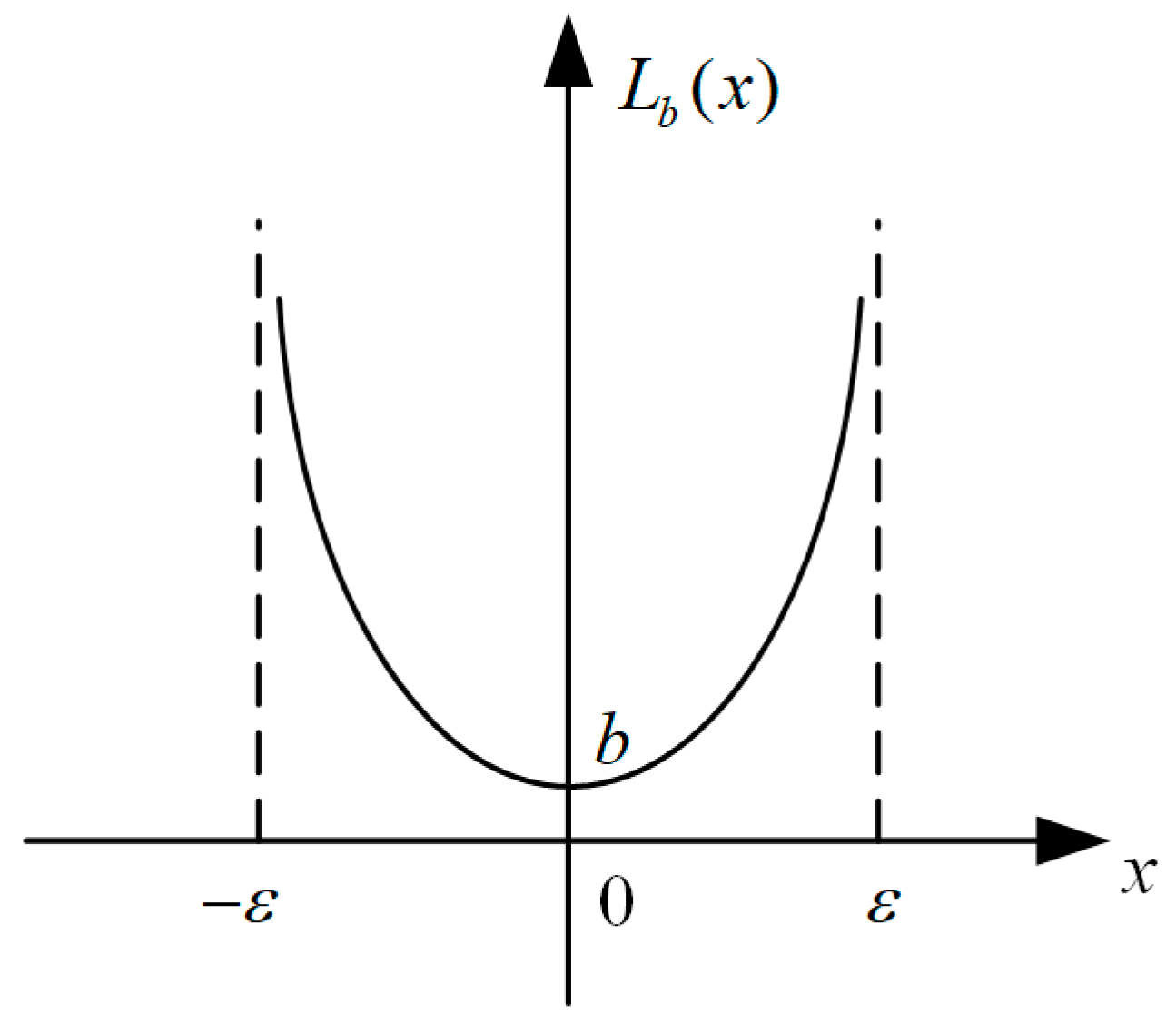
where $\mathbf{\varpi }(z_2)$ is a saturation function given by:

$$\mathbf{\varpi }(z_2)=\frac{z_2}{\Vert z_2\Vert }\min (\Vert z_2\Vert ,1)$$

(38)

The time derivate of (37) can be formulated as:

$$V^{\prime }=\frac{z_1\circ {z^{\prime }}_1}{1+2C_0{\Vert z_1\Vert }^2}+z_2\circ z^{\prime }-\frac{{z^{\prime }}_1\circ \mathbf{\varpi }(z_2)}{4(1+2C_0\Vert z_1\Vert )}-\frac{{\mathbf{\varpi }}^{\prime }(z_2)\circ z_1\circ \ln (1+2C_0\Vert z_1\Vert )}{8C_0\Vert z_1\Vert }$$

(39)

$$V^{\prime }\le -\frac{1}{2}{\Vert z_1\Vert }^{1/2}-\Vert z_2\Vert \circ \left(\frac{1}{4}-\frac{M}{b^2(1+2C_0\Vert z_1\Vert )}\right)+{\mathbf{\varpi }}^{\prime }(z_2)\circ \frac{M}{8b^2{C}_0}\circ \frac{\ln (1+2C_0\Vert z_1\Vert )}{1+2C_0\Vert z_1\Vert }$$

(40)

For the Lyapunov function (37), the following inequality exists:

$$\frac{3\ln (1+2C_0\Vert z_1\Vert )}{8C_0}+\frac{z_2^2}{2}\le V\le \frac{5\ln (1+2C_0\Vert z_1\Vert )}{8C_0}+\frac{z_2^2}{2}$$

(41)

Consequently, $V$ is positive-definite. Then the theorem will be proved if the following expression is true:

$$\lim {\sup }_{t\to \infty }V\le V^{*}$$

(42)

It can be concluded that (42) holds true when $V^{*}$ satisfies:

$$V^{*}=\frac{16M^2}{b^4}+\frac{5\ln (1+8(4M/b^2-1/8))}{4C_0}$$

(43)

This completes the proof. □

4. Simulation

In this section, we designed three simulation examples to discuss the effectiveness and the robustness of the proposed guidance law. First, various desired terminal angles are taken into consideration to demonstrate its nice performance. Next, in order to test the robustness, a Monte Carlo method with uncertain input parameters is utilized. Finally, the proposed guidance law is compared with other guidance laws under two different cases. The whole simulations are supported by the MATLAB platform, and a fourth-order Runge–Kutta solver is used throughout the simulations.

4.1. Simulation Set-Up

Considering the limited capacity of the real actuator, the lateral acceleration of the missile can be formulated as:

$$a_M=\{\begin{array}{ll}{a}_{M,\max }sign\left(a_M\right),\hfill & \left|a_M\right|\ge a_{M,\max }\hfill \\ a_M,\hfill & \left|a_M\right|<a_{M,\max }\hfill \end{array}$$

(44)

where $a_{M,\max }$ is the ultimate maximum lateral acceleration, and we denote that $a_{M,\max }=300 {\mathrm{m}/\mathrm{s}}^2$. In order to avoid the discontinuity problem of the sign function sign(x), a sigmoid function is utilized instead in this paper, which is given by:

$$sigmoid(x)=\frac{2}{1+e^{-x}}-1$$

(45)

In addition, the simulation examples in this paper are set up as follows: (1) the initial missile-target engagement condition: $r_0=8000 \mathrm{m}$, ${\dot{r}}_0=-800 \mathrm{m}/\mathrm{s}$, ${\theta }_0={30}^{\circ }$, ${\varphi }_0={10}^{\circ }$, ${\dot{\theta }}_0={\dot{\varphi }}_0=0^{\circ }/\mathrm{s}$, ${\theta }_d={45}^{\circ }$ and ${\varphi }_d={25}^{\circ }$; (2) the target maneuvering condition: $a_{T\theta }=a_{T\varphi }=-30 {\mathrm{m}/\mathrm{s}}^2$, and $a_{Tr}=0 {\mathrm{m}/\mathrm{s}}^2$; (3) the parameters of sliding mode manifold and barrier function-based super-twisting controller are given in

Table 1. The parameters of sliding mode manifold and barrier function-based super-twisting controller.

Parameter	Value	Parameter	Value
$k_1$	0.5	$l_{10}$$,l_{20}$	0.1
$k_2$	0.1	$l_{11}$$,l_{21}$	1
$k_3$	2.5	${\epsilon }_1$	0.1
$\xi$	0.2	${\epsilon }_2$	0.1

; (4) the fixed step size of the fourth-order Runge–Kutta solver is 0.001 s.

4.2. Simulation for Different Terminal Angles

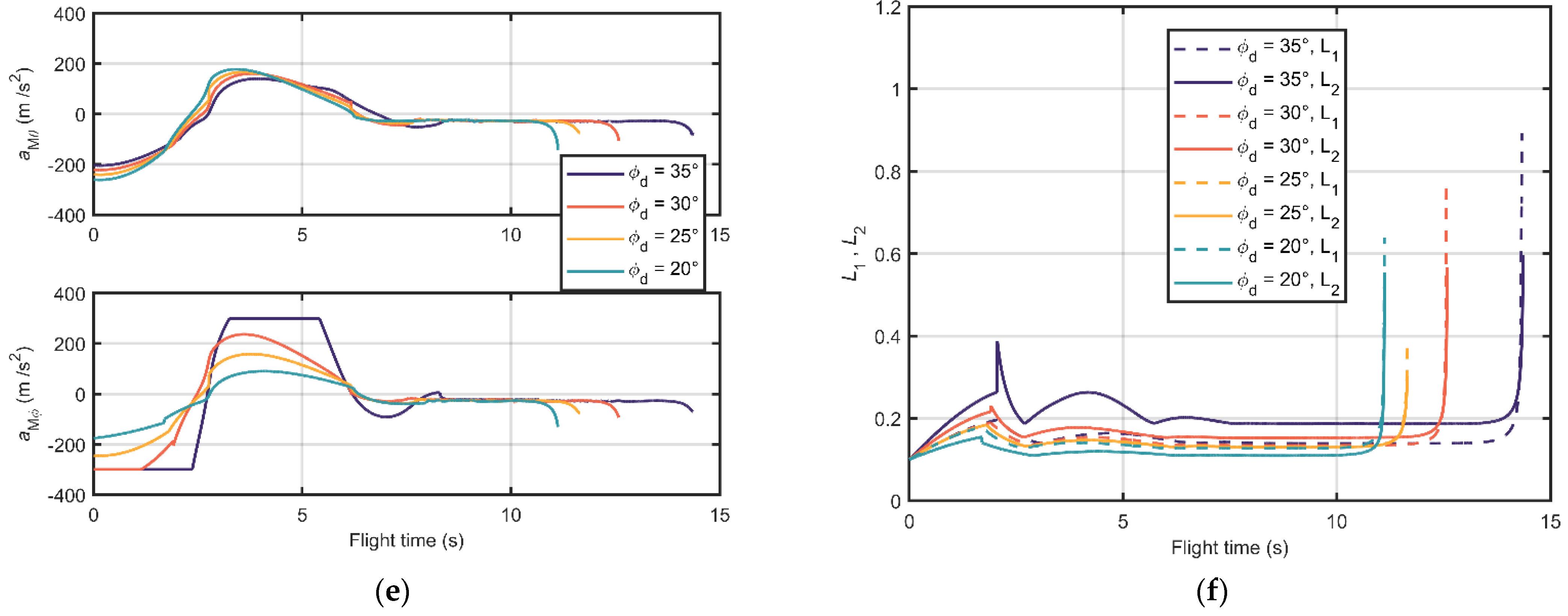
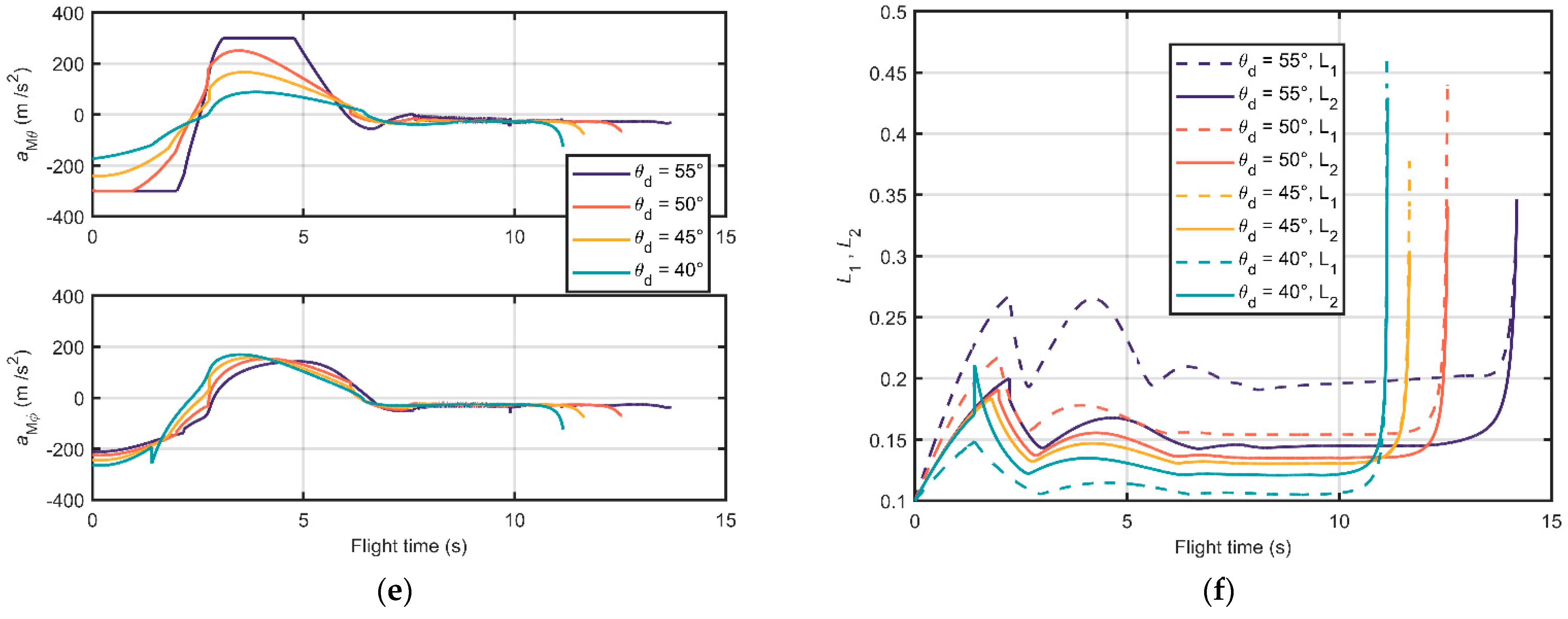
The proposed multivariable barrier function-based super-twisting guidance law is expected to have a nice performance under different desired terminal angles. In order to test this property, a simulation with various desired terminal angles is investigated.

Let the desired terminal angles ${\varphi }_d={35}^{\circ },{30}^{\circ },{25}^{\circ }$ and ${20}^{\circ }$, when the azimuth angle ${\theta }_d={45}^{\circ }$; ${\theta }_d={55}^{\circ },{50}^{\circ },{45}^{\circ }$ and ${40}^{\circ }$, when the elevation angle ${\varphi }_d={25}^{\circ }$. Other parameters are set up in Section 4.1.

Figure 3 and Figure 4 show the simulation results. Figure 3a and Figure 4a illustrate the relative trajectories between missile and target in the inertial coordinate system when the desired terminal LOS angles are ${\varphi }_d={35}^{\circ },{30}^{\circ },{25}^{\circ },{20}^{\circ }$ and ${\theta }_d={55}^{\circ },{50}^{\circ },{45}^{\circ },{40}^{\circ }$, respectively. All the trajectories under the simulation conditions could converge to zero, which testify that missiles can catch up with the target in finite time utilizing the designed guidance law in this paper. Figure 3b and Figure 4b show the change of elevation angle and azimuth angle during the flight time under the two designed scenarios, respectively. The missile with the proposed guidance law can reach the desired terminal angle before meeting the target and then keep on it. This implies the proposed guidance law has the nice property of terminal angle constraint. The elevation and azimuth angular rates are shown in Figure 3c and Figure 4c. One can conclude that a wider margin between the initial LOS angle and the desired terminal angle will lead to a larger LOS angular rate and shorter convergence time. Remarkably, when the missile approaches the target, or $r\to 0$, $\ddot{\theta }$ and $\ddot{\varphi }$ will change significantly due to the form of Equation (4). Hence there are drops at the end of the flight time in Figure 3b,c and Figure 4b,c. Figure 3d and Figure 4d illustrate the trends of extraneous LOS angles and LOS angular rates of the two scenarios, respectively. There are no distinct gaps between the trends. The acceleration histories are shown in Figure 3e and Figure 4e, from which we can conclude that there is no distinct chattering during the flight time in these simulation conditions. Moreover, Figure 3f and Figure 4f demonstrate the adaptive gains. The time variables reach the switch point $t=\overline{t}(s_0)$ around 2 s, which results in leaps of the gains at that time.

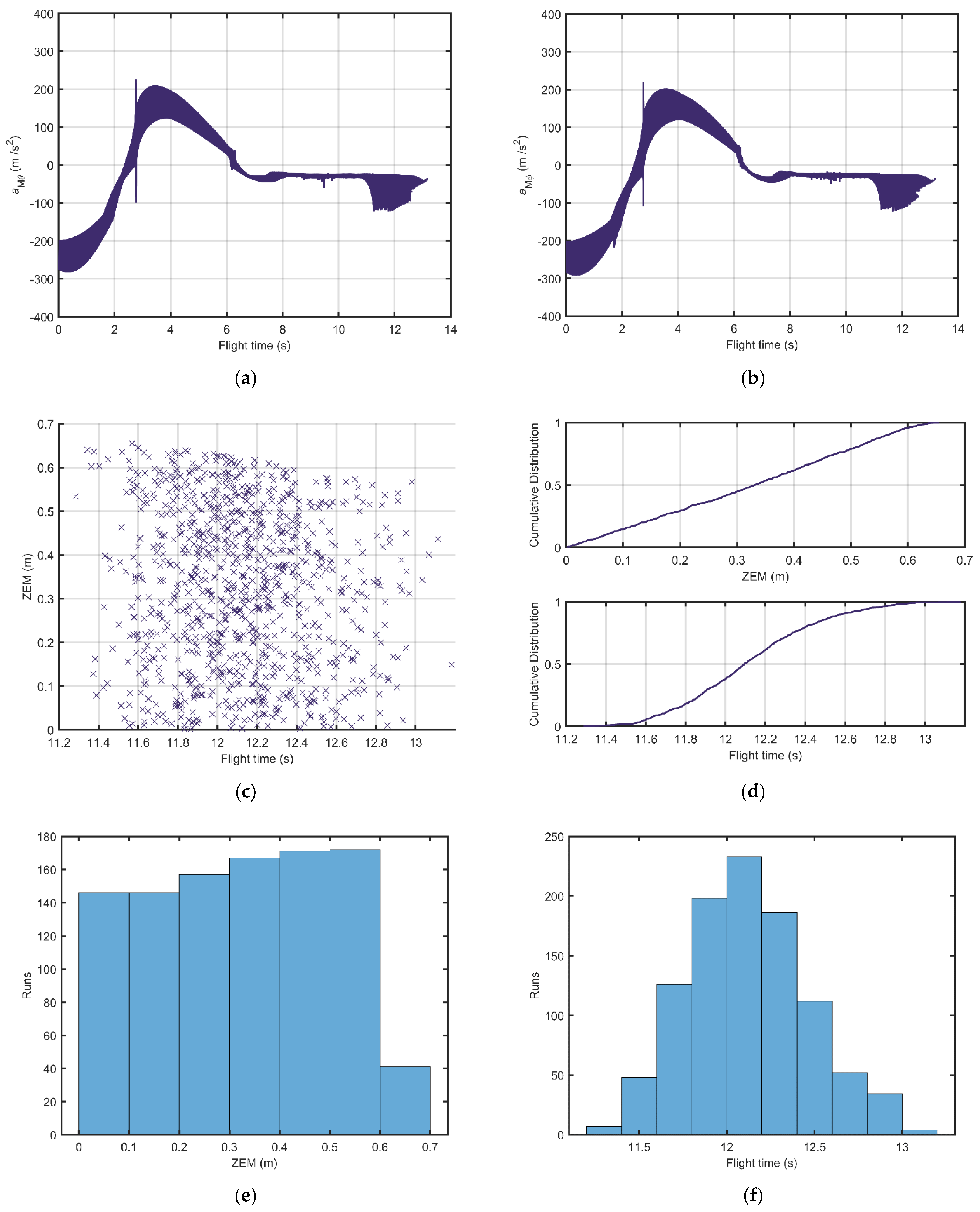
4.3. Simulation Based on Monte Carlo Method

To demonstrate the robustness of the proposed guidance law, a Monte Carlo simulation example with 1000 runs is performed. Considering the uncertainty of the initial relative velocity and the measurement errors of LOS angles, set up the Monte Carlo simulation parameters as: ${\dot{r}}_0=\left[-825 \mathrm{m}/\mathrm{s}, -775 \mathrm{m}/\mathrm{s}\right]$, ${\theta }_0=\left[{25}^{\circ },{35}^{\circ }\right]$, ${\varphi }_0=\left[5^{\circ },{15}^{\circ }\right]$. The general dynamical environment is the same as that introduced in Section 4.1. Thus, other initial conditions and parameters remain the same as in Section 4.1. In every run of this Monte Carlo simulation, the simulation parameters ${\dot{r}}_0$, ${\theta }_0$ and ${\varphi }_0$ are selected randomly from the given interval by the random function of MATLAB.

The results of the Monte Carlo simulation example are shown in Figure 5. Figure 5a,b illustrate the output acceleration commands along LOS coordinate axes $\theta$ and $\varphi$, respectively. The acceleration curves have a stable range and trend, which implies that the proposed guidance law could address uncertainty problems and have nice robustness. Remarkably, some curves have distinct leaps around 3 s in Figure 5a,b. The reason for this phenomenon is that most runs of the Monte Carlo simulation reach the switch points of the super-twisting gains around 2 s, then the changings of the gains lead to dramatic outputs of accelerations in some runs. Figure 5c is the scatter diagram of zero-effort miss (ZEM) distance with respect to flight time. Moreover, Figure 5d depicts the cumulative distribution function curves of ZEM and flight time, respectively. In addition, the bar graphs of the numbers of Monte Carlo runs with respect to ZEM and flight time is illustrated in Figure 5e,f, respectively. In this example, we find that the ZEMs are smaller than 0.7 m; and the range of flight time is [11.2 s, 13.2 s]. Moreover, the distributions of ZEM and flight time are similar to uniform distribution and normal distribution, respectively.

4.4. Simulation Compared with Other Super-Twisting Guidance Laws

Compared with a classical super-twisting controller, the barrier function-based controller does not need the information of the upper bound of disturbance and the super-twisting state variable $y(t)$ of it can converge fast. To further verify the distinguished property of the proposed barrier function-based guidance law, two other kinds of super-twisting guidance laws are considered. The first is a fixed-gain super-twisting (FGST) guidance law, which is given by [31]:

$$\{\begin{array}{l}{a}_M=-B^{-1}(\overline{F}(x)+c_1\frac{s}{{\Vert s\Vert }^{1/2}}-c_{2}s-y(t))\hfill \\ \dot{y}(t)=-c_3\frac{s}{\Vert s\Vert }-c_{4}s\hfill \end{array}$$

(46)

where $c_i,i=1,2,3,4$ is positive constant, it is selected as $c_1=1.6$, $c_2=0.1$, $c_3=0.4$ and $c_4=0.1$ in this paper.

The second is an equivalent control based super twisting (ECST) guidance law, which has the following expression [32]:

$$\{\begin{array}{l}{a}_M=-B^{-1}(\overline{F}(x)+d_1\sqrt{\overline{L}}\circ \frac{s}{{\Vert s\Vert }^{1/2}}-d_2(t)\overline{L}\circ s-y(t))\hfill \\ \dot{y}(t)=-d_3(t)\overline{L}\circ \frac{s}{\Vert s\Vert }-d_4(t){\overline{L}}^2\circ s\hfill \end{array}$$

(47)

where $\overline{L}$ is a dual-layer gain, its detailed expression is given in Appendix A; $d_i,i=1,2,3,4$ is positive constant, it is selected as $d_1=5$, $d_2=0.1$, $d_3=1.2$ and $d_4=1$ in this paper.

In order to further demonstrate the effectiveness and applicability of the proposed guidance law, the comparison simulation is designed to contain two cases with various target maneuvers:

• The target accelerations in LOS coordinate $a_{T\theta }=a_{T\varphi }=-30(2\pi t){\mathrm{m}/\mathrm{s}}^2$;
• The target accelerations in LOS coordinate $a_{T\theta }=a_{T\varphi }=-30{\mathrm{m}/\mathrm{s}}^2$.

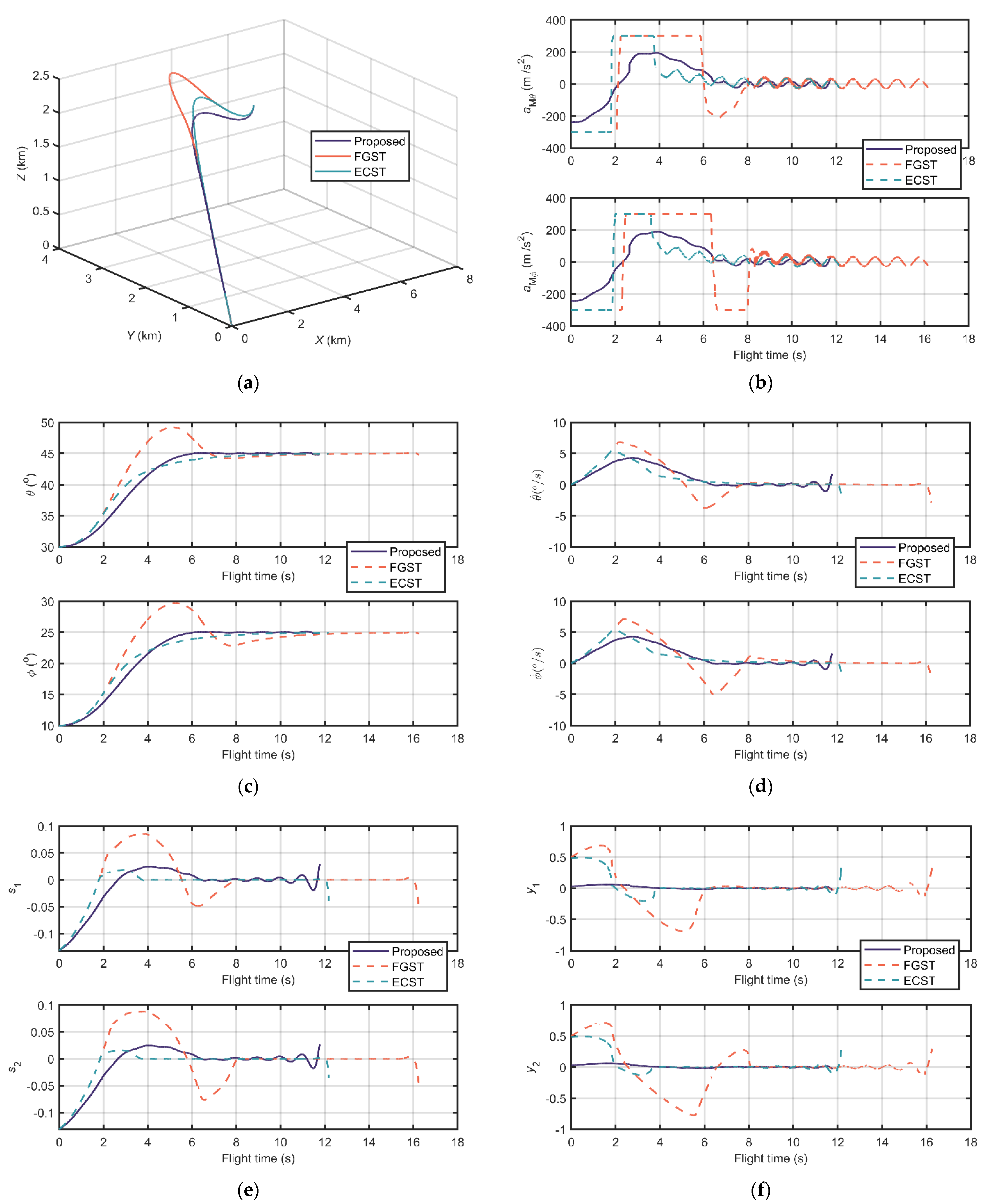
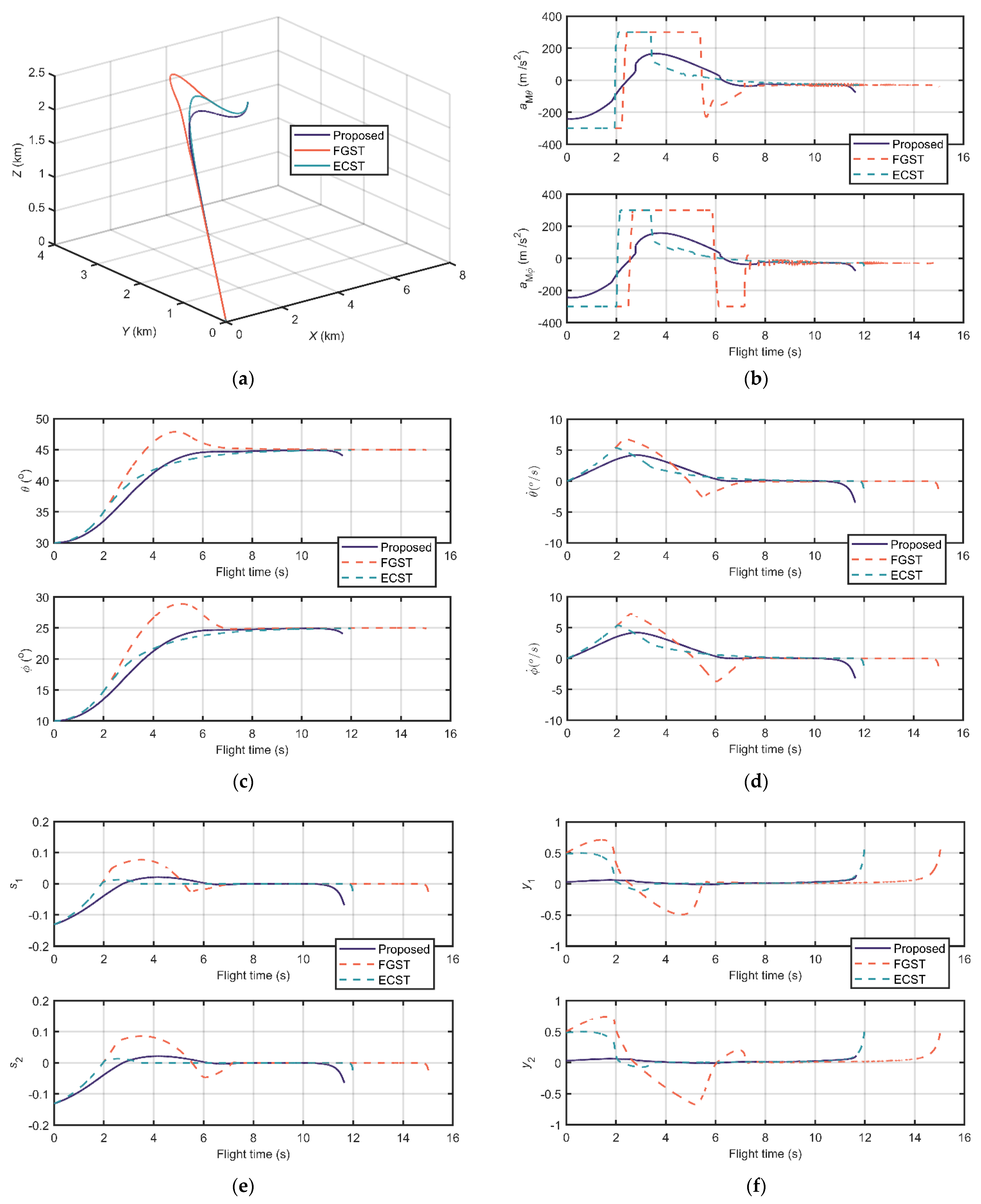
The other initial parameters of these two scenarios are the same as those in Section 4.1. Figure 6 and Figure 7 demonstrate the comparison results of case 1 and case 2, respectively. Figure 6a and Figure 7a show the relative distance trajectories between missile and target. It can be clearly seen that the trajectories of the three guidance laws can all converge to zero. Moreover, the curves of the proposed are shorter than others. Figure 6b and Figure 7b depict the acceleration commands. It can be noticed that the acceleration commands of FGST and ECST reach the ultimate maximum lateral acceleration during the flight time. Moreover the command curves of FGST have distinct chattering. Contrarily, the curve of the proposed has smaller maximum values and smooth properties. The LOS angles are illustrated in Figure 6c and Figure 7c, and the LOS angular rates are illustrated in Figure 6d and Figure 7d, respectively. The LOS angles of the proposed reach the desired angles faster than the others. Moreover, its angular rates have smaller sizes in the vicinity of zero. The sliding variables of the two cases are shown in Figure 6e and Figure 7e, respectively, which all converge to zero in finite time. Figure 6f and Figure 7f show the convergence of super-twisting state variable $y(t)$. It is obvious that the range values to which the proposed guidance law converges are much smaller than the others in these cases.

Furthermore, the detailed information of the two cases is listed in

Table 2. Simulation results of case 1.

Guidance Law	Flight Time	$\mathbf{Maximum}\mathbf{of}\left|{\mathit{a}}_{\mathit{M}\mathit{\varphi }}\right|$	$\mathbf{Duration}\mathbf{of}{\mathit{a}}_{\mathit{M}\mathit{\varphi },\mathbf{max}}$	$\mathbf{Error}\mathbf{of}\mathit{\varphi }$	$\mathbf{Interval}\mathbf{of}{\mathit{y}}_2$
Proposed	11.77 s	243 m/s2	None	0.11°	[−0.02, 0.06]
FGST	16.25 s	300 m/s2	8.01 s	0.14°	[−0.85, 0.72]
ECST	12.18 s	300 m/s2	3.57 s	0.25°	[−0.14, 0.49]

and

Table 3. Simulation results of case 2.

Guidance Law	Flight Time	$\mathbf{Maximum}\mathbf{of}\left|{\mathit{a}}_{\mathit{M}\mathit{\varphi }}\right|$	$\mathbf{Duration}\mathbf{of}{\mathit{a}}_{\mathit{M}\mathit{\varphi },\mathbf{max}}$	$\mathbf{Error}\mathbf{of}\mathit{\varphi }$	$\mathbf{Interval}\mathbf{of}{\mathit{y}}_2$
Proposed	11.66 s	241 m/s2	None	0.90°	[0, 0.11]
FGST	15.03 s	300 m/s2	7.16 s	0.11°	[−0.67, 0.74]
ECST	11.99 s	300 m/s2	3.38 s	0.13°	[−0.07, 0.58]

, respectively. It can be obviously seen that the flight time of missiles utilizing the proposed guidance law is the shortest compared with the ones using FGST and ECST. In addition, the acceleration commands $\left|a_{M\varphi }\right|$ of FGST and ECST reach the ultimate maximum lateral acceleration $a_{M\varphi ,\max }$ during the flight time, which sustain 8.01 s and 3.57 s (case 1), and 7.16 s and 3.38 s (case 2), respectively. Contrarily, the maximum acceleration commands $\left|a_{M\varphi }\right|$ of the proposed algorithm are less than 300 m/s² so that the actuator using the proposed guidance law is more agile and flexible. As for the errors of terminal LOS angle $\varphi$ of the two cases, there is little distinction among the guidance laws with these three super-twisting methods. Moreover, the super-twisting state variables $y_2$ of the proposed converge to smaller vicinities of zero in these two cases, which have intervals of [−0.02,0.06] and [0,0.11], respectively.

5. Conclusions

This paper presents a novel multivariable barrier function-based super-twisting guidance law, which has the following distinguished properties:

• Under the simulation condition given in Section 4.1, missiles using the proposed guidance law can achieve high guidance accuracy (ZEMs are smaller than 0.7 m) and high terminal angle accuracy (angle errors are smaller than 1°) in a short flight time;
• The guidance law can maintain its distinguished performance in different scenarios of various target accelerations;
• With the uncertainty of the missile dynamics and the measurement, the guidance law has a remarkable property of robustness.

Moreover, compared with other sliding mode and super-twisting guidance laws, the one proposed in this paper does not require the information of the disturbance derivatives. The chattering of the acceleration commands is eliminated. Furthermore, the designed super-twisting gains are smaller, which lead to smaller super-twisting state variables and smaller acceleration commands. Following the increasing or decreasing of the disturbances, the gains are also sufficient to offset the disturbances and keep on the sliding mode during the control progress, which demonstrates a better property of robustness.