Systematic Error Correction for Geo-Location of Airborne Optoelectronic Platforms

Abstract

In order to improve the geo-location accuracy of the airborne optoelectronic platform and eliminate the influence of assembly systematic error on the accuracy, a systematic geo-location error correction method is proposed. First, based on the kinematic characteristics of the airborne optoelectronic platform, the geo-location model was established. Then, the error items that affect the geo-location accuracy were analyzed. The installation error between the platform and the POS was considered, and the installation error of platform’s pitch and azimuth was introduced. After ignoring higher-order infinitesimals, the least square form of systematic error is obtained. Therefore, the systematic error can be obtained through a series of measurements. Both Monte Carlo simulation analysis and in-flight experiment results show that this method can effectively obtain the systematic error. Through correction, the root-mean-square value of the geo-location error have reduced from 45.65 m to 12.62 m, and the mean error from 16.60 m to 1.24 m. This method can be widely used in systematic error correction of relevant photoelectric equipment.

1. Introduction

Airborne optoelectronic platforms, which can realize a wide range of search, identification, tracking and measurement tasks, are playing an increasingly important role in military and civilian applications such as search, rescue of the wounded and target reconnaissance, etc. [1,2,3,4]. The process of obtaining geographic coordinate information of a target using an airborne optoelectronic platform is called geo-location. Accurate geo-location is of great significance to the rescue of the wounded, target reconnaissance, etc. In recent years scholars have conducted extensive research on geo-location algorithms. The following methods are used to improve the geo-location accuracy:

(1)

Build a more accurate model based on the Earth ellipsoid model or digital elevation model. For example, Stich proposed a geo-location algorithm based on the Earth ellipsoid model from a single image using an aerial camera to reduce the influence of the Earth’s curvature on the positioning result [5]. Qiao proposed a geo-location algorithm based on the digital elevation model (DEM) for an airborne wide-area reconnaissance system, and the simulation results show that the proposed algorithm can improve the geo-location accuracy of ground target in rough terrain area [6]. The Global Hawk unmanned aerial vehicle (UAV) geo-location system is also based on an Earth ellipsoid model to calculate the geodetic coordinates of the image center [7].

(2)

Image the target multiple times or using multiple sensors or multiple UAVs to get redundant information to improve geo-location accuracy. Bai proposed an improved two-UAV intersection localization system based on airborne optoelectronic platforms using the crossed-angle localization method to address the limitation of the existing UAV photoelectric localization method used for moving objects [8]. Lee proposed an information-sharing strategy by allocating sensors to multiple small UAVs to solve the drawbacks that a small unmanned aerial vehicle (UAV) cannot be equipped with many sensors for target localization [9]. Morbidi and Mariottini described an active target-tracking strategy to deploy a team of UAVs along the paths that minimize the uncertainty about the position of a moving target [10]. Qu proposed a ground target cooperative geometric localization method based on the locations of several unmanned aerial vehicles (UAVs) and their relative distances from a target, and simulation results from the MATLAB/Simulink toolbox show that this method is more effective than a traditional approach [11].

(3)

Use filtering algorithms or video sequences to optimize positioning results. Zhao et al. [12] proposed an adaptive tracking algorithm based on the Kalman filter (KF). Qiao proposed a moving average filtering (MAF) to improve the geo-location accuracy of moving ground target, which adapts to both constant velocity motion model and the turn model [6]. Wang proposed a recursive least squares (RLS) filtering method based on UAV dead reckoning to improve the accuracy of the multi-target localization [13]. Nonlinear filter [14,15,16,17] and methods based on video sequence [18,19,20,21,22,23] are also proposed to estimate the locations of targets.

(4)

Analyze the factors causing the error and use calibration methods to make corrections. Liu proposed a system and method for correction of relative angular displacements between an unmanned aerial vehicle (UAV) and its onboard strap-down photoelectric platform to improve localization accuracy [24]. With the Lens distortion parameter obtained in the laboratory, Wang proposed a real-time zoom lens distortion correction method to improve the accuracy of the multi-target localization [13].

In all the above references, the authors either didn’t take into account the effect of the systematic error [4,19,24,25], or just introduced it as a fixed bias [6,8]. Eliminating systematic error is the basis for improving the accuracy of target geo-location since it directly affects the geo-location accuracy and the filtering algorithms [6,13,14,15,16,17] cannot eliminate systematic error. The geo-location error will increase along with the increase of the distance to the target with systematic error. At a certain distance, it will become the main error that affects the geo-location accuracy. So, eliminating the systematic error is of great significance to improve the accuracy of geo-location.

The method proposed here is one kind of boresight calibration. However, it is different from those methods. First, boresight calibration methods usually solve the misalignments between the image coordinate system and the body coordinate system established by the inertial instruments [26,27]. While this method mainly focuses on airborne optoelectronic platform which always has additional rotation axes such as azimuth and pitch axes. Secondly, the transformations are usually established for various photogrammatic bundle adjustment systems [26,27,28]. While this method establishes those transformations through the distance measured by the laser rangefinder and one target for each measurement, so the method proposed in this article is a special boresight calibration with more axes and a laser rangefinder to measure the distance between GCPs and the imaging system.

The primary contribution of this paper is that a geo-location systematic error correction method is proposed. This method has the following advantages:

This method can correct the systematic error from the manufacture and assemble which can’t be eliminated by laboratory equipment. For example, after the photoelectric payload is installed on the UAV, due to the size and other issues, it is difficult for the laboratory equipment to correct the installation error between the aircraft and the payload.

This method is easy to implement. Unlike the other laboratory methods [13,24], this method doesn’t need special equipment and the systematic error can be obtained through flight experiments and control points on the ground.

The rest of paper is organized as follows: Section 2.1 briefly presents the overall framework of the geo-localization system. Section 2.2 presents the reference frames and transformations required for the geo-location system. Section 2.3 presents the ground target geo-location model. Section 2.4 presents the geo-location error analysis and methods to get the systematic error using control points. Section 3 presents the results of systematic error correction methods from both Monte Carlo analysis and in-flight experiments. Section 4 presents the discussion and our conclusions are given in Section 5.

2. Materials and Methods

2.1. Overall Framework

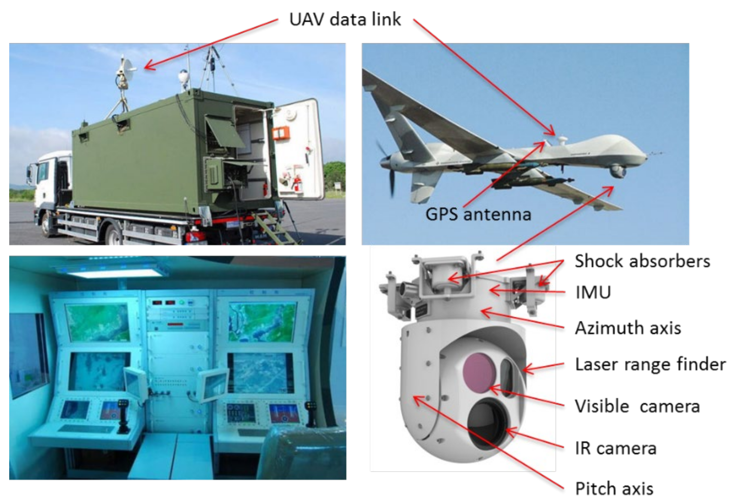
The geo-location system introduced in this article is composed of a ground control station, a digital and image transmission link and an UAV with an airborne optoelectronic platform, as shown in the Figure 1. The UAV was developed by Changchun Institute of Optics Fine Mechanics and Physics, Chinese Academy of Science for civilian applications such as rescue of the wounded and forest fire prevention. The ground control system is responsible for the control and status display of the UAV and the airborne optoelectronic platform. The transmission link is responsible for real-time downloading of video data. The airborne optoelectronic platform is composed of visible camera, Thermal imaging camera, laser rangefinder, stabilized platforms, image trackers, inertial measurement unit (IMU), etc. The stabilized platforms include the azimuth axis and the pitch axis, and each axis has an encoder which can output the current azimuth and pitch angle in real time.

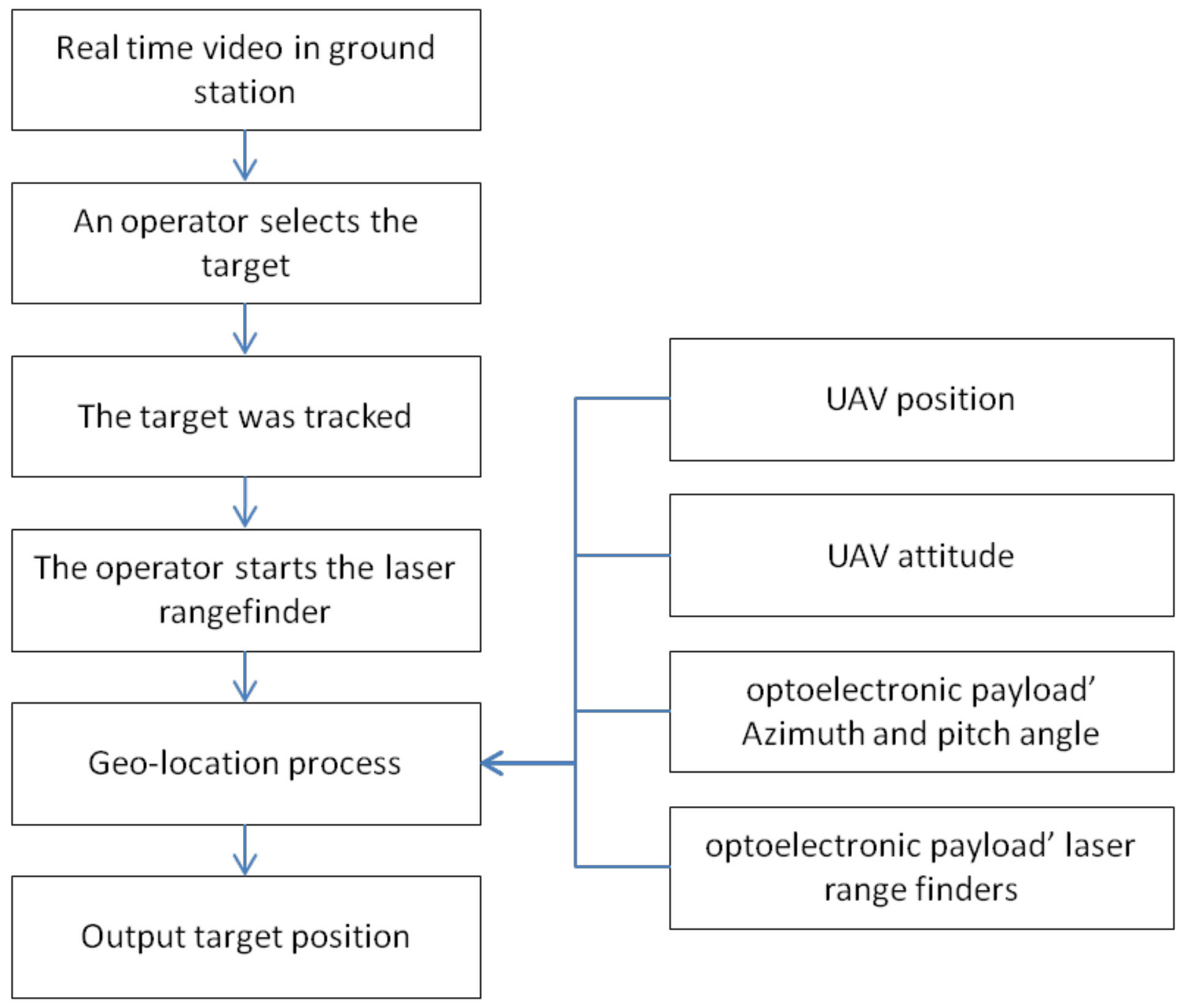
The geo-location process is shown in the Figure 2. First, an operator selects the target in the real-time video in the ground control station. Then when the airborne optoelectronic platform is tracking the selected target and the operator turns on the laser rangefinder, the airborne optoelectronic platform starts the geo-location process. The geo-location results of the target are sent to the ground control station for real-time display.

In fact, the geo-location process can realize the geo-location at any position in sight of the camera. In this article, in order to realize the correction of the systematic error, only the target at the center of the field of view is considered. Since the axis of the laser ranging is parallel to the axis of the cameras during the design and installation of the airborne optoelectronic platform, the laser rangefinders’ value is the distance between the target and the photoelectric payload.

2.2. Establishment of the Basic Coordinates

Four basic coordinate frames are used in the geo-location algorithm, including the imaging coordinate frame $V\left(X_v{Y}_v{Z}_v\right)$, the aircraft coordinate frame $B\left(X_b{Y}_b{Z}_b\right)$, the navigation coordinate frame $P\left(X_p{Y}_p{Z}_p\right)$ and the geodetic coordinate frame $G\left(X_g{Y}_g{Z}_g\right)$.

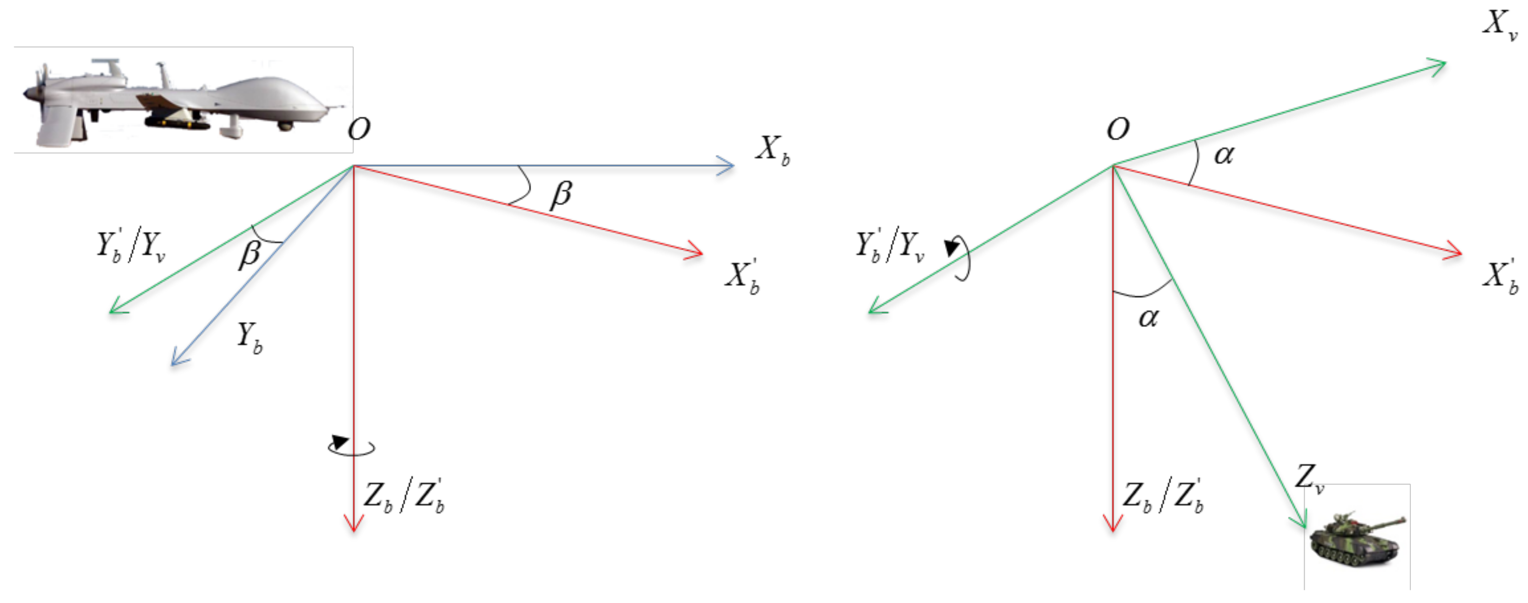
2.2.1. The Imaging Coordinate Frame $\mathrm{V}\left({\mathrm{X}}_{\mathrm{v}}{\mathrm{Y}}_{\mathrm{v}}{\mathrm{Z}}_{\mathrm{v}}\right)$

This frame has its origin at the rotation center of the payload. The $X_v$ axis points upwards if the camera is along vehicle x-axis, and the $Z_v$ axis is along the light of sight (LOS) of the imaging system and pointing to the target, and $Y_v$ forms an orthogonal right-handed frame set. This imaging system is installed in a two-axis’ gimbal, while the outer gimbal angle rotates around the $Z_b$ axis, represents the azimuth angle $\beta$, having the initial position as front, and positive to the right. The inner gimbal angle rotates around the $y_v$ axis, represents the pitch angle $\alpha$, having initial position as the LOS point down along the $Z_v$ axis and positive while rotate to the front. The imaging coordinate frame and the transition process between the imaging coordinate frame and aircraft coordinate frame are shown in Figure 3.

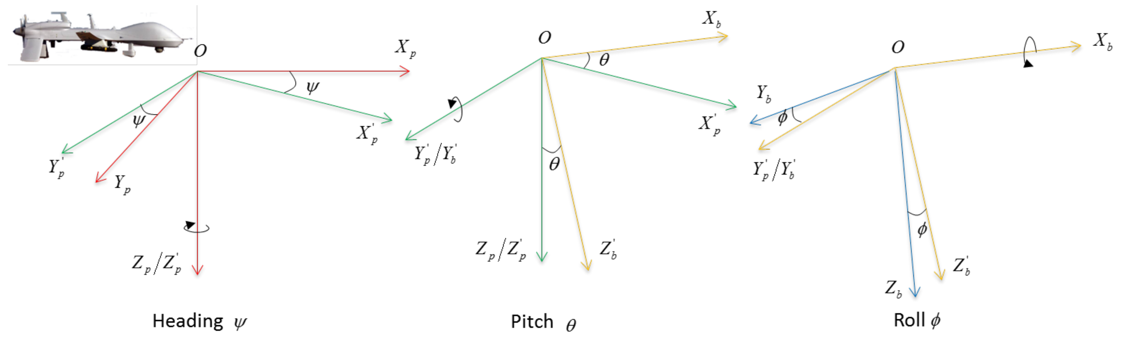
2.2.2. The Aircraft Coordinate Frame $\mathrm{B}\left({\mathrm{X}}_{\mathrm{b}}{\mathrm{Y}}_{\mathrm{b}}{\mathrm{Z}}_{\mathrm{b}}\right)$

This frame is the standard ARINC frame with origin shifted to the center of the optical platform center. The $X_b$ axis points to the nose of the aircraft, $Z_b$ axis points to the bottom of the aircraft, and $Y_b$ forms an orthogonal right-handed set. POS were mounted on this frame, and the roll, pitch and yaw angles $\left(\varphi ,\theta ,\psi \right)$ rotate around the $X_b$ axis, $Y_b$ axis and $Z_b$ axis. The aircraft coordinate frame and the transition between the aircraft coordinate frame and navigation coordinate frame are shown in Figure 4.

2.2.3. The Navigation Coordinate Frame $\mathrm{P}\left({\mathrm{X}}_{\mathrm{p}}{\mathrm{Y}}_{\mathrm{p}}{\mathrm{Z}}_{\mathrm{p}}\right)$

This frame is the standard NED (north, east, down) reference frame and has its origin at the aircraft’s center; the $X_p$ axis points to true north, $Y_p$ axis points to the east, and $Z_p$ axis lies along the local geodetic vertical and is positive down. The transition between the geodetic coordinate frame and the navigation coordinate frame is shown in Figure 5.

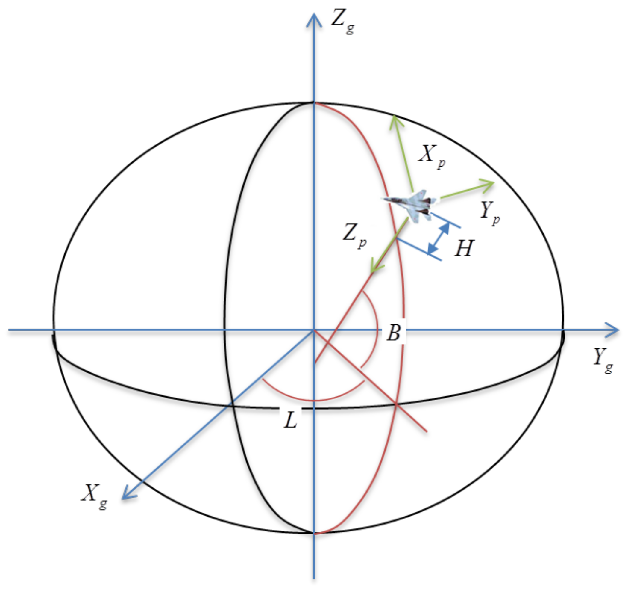
2.2.4. The Geodetic Coordinate Frame $\mathrm{G}\left({\mathrm{X}}_{\mathrm{g}}{\mathrm{Y}}_{\mathrm{g}}{\mathrm{Z}}_{\mathrm{g}}\right)$

This frame is defined in WGS-84 and has its origin at the Earth’s geometric center. The $X_g$ is in the equatorial plane at the prime meridian, $Z_g$ points north through the polar axis, and $Y_g$ forms an orthogonal right-handed set. The elliptical Earth model can be expressed as Figure 5:

$$\frac{x_g^2}{R_E^2}+\frac{y_g^2}{R_E^2}+\frac{z_g^2}{R_P^2}=1$$

(1)

where $R_E=6,378,137 \mathrm{m}$ is the semi-major axis and $R_P=6,356,752 \mathrm{m}$ is the semi-minor axis.

The geographical position of a point can be expressed as the longitude, latitude, and geodetic height (B, L, and H). The point in the geodetic coordinate frame can be expressed as:

$$P_g=\left[\begin{array}{c}{x}_g\\ y_g\\ z_g\end{array}\right]=\left[\begin{array}{c}\left(R_N+H\right) \cos B \cos L\\ \left(R_N+H\right) \cos B \sin L\\ \left[R_N\left(1-e^2\right) +H\right]\sin B \end{array}\right]$$

(2)

where $e=\sqrt{\frac{R_E^2-R_P^2}{R_E}}$ the first eccentricity of the Earth ellipsoid is, $R_N=\frac{R_E}{\sqrt{1-e^{2}si{n}^{2}B}}$ is the prime vertical of curvature.

2.3. Ground Target Geo-Location

When the airborne optoelectronic platform in the initial position, azimuth $\beta$ and pitch $\alpha$ angle both equal to zero, and the imaging coordinate frame coincides with the aircraft coordinate frame. The matrix transforms from the frame $V\left(X_v{Y}_v{Z}_v\right)$ to the frame $B\left(X_b{Y}_b{Z}_b\right)$ can be expressed as:

$$M_b^v=\left[\begin{array}{ccc}\cos \beta & -\sin \beta & 0\\ \sin \beta & \cos \beta & 0\\ 0& 0& 1\end{array}\right]·\left[\begin{array}{ccc}\cos \alpha & 0& \sin \alpha \\ 0& 1& 0\\ -\sin \alpha & 0& \cos \alpha \end{array}\right]$$

(3)

The position and orientation system (POS), which is composed of the global positioning system (GPS) and inertial measurement unit, can measure the position and attitude information of the airborne platform accurately. The position information of the airborne optoelectronic platform includes the latitude, longitude, and height $\left(B,L,H\right)$ and the attitude information includes roll, pitch and yaw angles $\left(\varphi ,\theta ,\psi \right)$. The matrix transforms from the frame $B\left(X_b{Y}_b{Z}_b\right)$ to the frame $P\left(X_p{Y}_p{Z}_p\right)$ can be expressed as:

$$M_p^b=\left[\begin{array}{ccc}\cos \psi & -\sin \psi & 0\\ \sin \psi & \cos \psi & 0\\ 0& 0& 1\end{array}\right]·\left[\begin{array}{ccc}\cos \theta & 0& \sin \theta \\ 0& 1& 0\\ -\sin \theta & 0& \cos \theta \end{array}\right]·\left[\begin{array}{ccc}1& 0& 0\\ 0& \cos \varphi & -\sin \varphi \\ 0& \sin \varphi & \cos \varphi \end{array}\right]$$

(4)

The matrix transforms from the frame $P\left(X_p{Y}_p{Z}_p\right)$ to the frame $G\left(X_g{Y}_g{Z}_g\right)$ can be expressed as:

$$M_g^p=\left[\begin{array}{ccc}\cos L& -\sin L& 0\\ \sin L& \cos L& 0\\ 0& 0& 1\end{array}\right]·\left[\begin{array}{ccc}\cos \left(-B-0.5\pi \right)& 0& \sin \left(-B-0.5\pi \right)\\ 0& 1& 0\\ -\sin \left(-B-0.5\pi \right)& 0& \cos \left(-B-0.5\pi \right)\end{array}\right]$$

(5)

and the matrix transform from frame imaging coordinate frame to the geodetic coordinate frame can be expressed as:

$$M_g^v=M_g^p·M_p^b·M_b^v$$

(6)

The distance ($Rng$) between the airborne platform and the target can be provided by the laser range finder. Since the laser beam is parallel with the LOS, the vector from the imaging system to the target can be expressed in geodetic coordinate frame as:

$$\overrightarrow{R_g}=M_g^v·{\left[\begin{array}{ccc}0& 0& Rng\end{array}\right]}^T$$

(7)

Then the target position $\overrightarrow{T_g}$ in geodetic coordinate frame can be expressed as:

$$\overrightarrow{T_g}=\overrightarrow{P_g}+\overrightarrow{R_g}$$

(8)

where $\overrightarrow{P_g}$ is a shift of origin from the center of gravity of the aircraft to the origin of the imaging system coordinate frame.

According to the elliptical Earth model, the latitude, the longitude and the geodetic height of the target can be solved according to [6]. The latitude of the northern hemisphere is positive, the latitude of the southern hemisphere is negative, and the target latitude and the geodetic height can be solved by the following iteration equations:

$$\begin{array}{l}\{\begin{array}{l}{R}_0=R_E\\ H_0=\sqrt[2]{x_g^2+y_g^2+z_g^2}-\sqrt[2]{R_E{R}_P}\\ B_0=\mathrm{atan}\left[\frac{z_g}{\sqrt[2]{x_g^2+y_g^2}}·{\left(1-\frac{e^2{R}_0}{R_0+H}\right)}^{-1}\right]\end{array}\\ \{\begin{array}{l}{R}_{k+1}=\frac{R_E}{\sqrt[]{1-e^2{\sin }^2{B}_k}}\\ H_{k+1}=\frac{\sqrt[]{x_g^2+y_g^2}}{\cos B_k}-R_k\\ B_{k+1}=\mathrm{atan}\left[\frac{z_g}{\sqrt[]{x_g^2+y_g^2}}·{\left(1-\frac{e^2{R}_{k+1}}{R_{k+1}+H}\right)}^{-1}\right]\end{array}\end{array}$$

(9)

According to the elliptical Earth model, the longitude of the eastern hemisphere is positive, the longitude of the western hemisphere is negative, and the target longitude can be solved by the following equation:

$$L=\left\{\begin{array}{ll}l& x_g>0\\ l+\pi ,& x_g<0,l<0\\ l-\pi ,& x_g<0,l>0\end{array}\right.,\hspace{1em}l=\mathrm{atan}\frac{y_g}{x_g}$$

(10)

2.4. Ground Target Geolocation Error Analysis and Systematic Error Correction

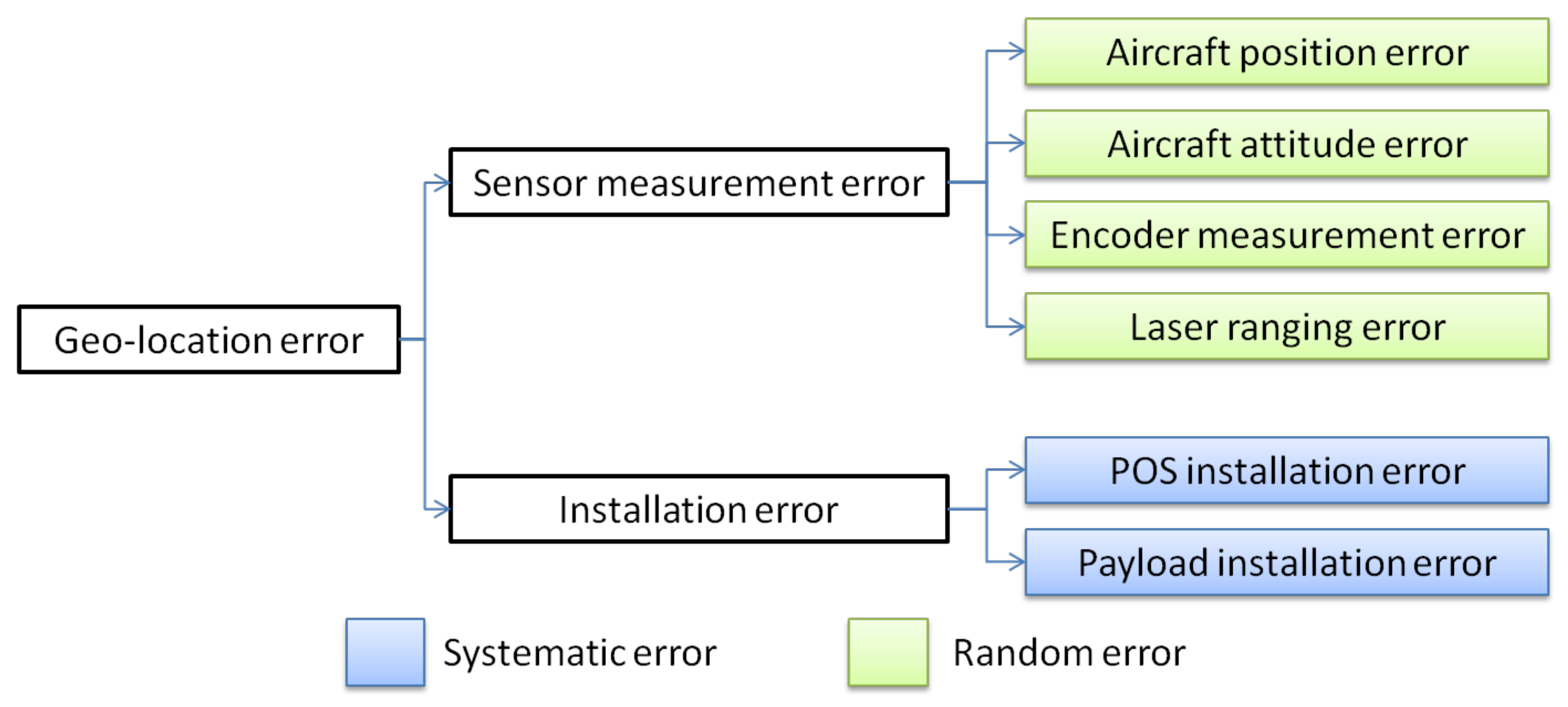
2.4.1. Analysis of Errors Affecting Geo-Location

Geo-location accuracy is an important factor that measures the ability of airborne optoelectronic platform to obtain target geographic location information. Therefore, it is very important to analyze the individual sources of measurement uncertainty of each part on geo-location process. Sensor measurement errors and installation errors are two major factors that affect the geo-location accuracy. For this platform, the position and attitude errors of the aircraft are mainly derived from the measurement errors of the integrated navigation system. The azimuth and pitch angle errors of the platform are derived from the measurement errors of the encoders, and the laser ranging errors are derived from the measurement errors of the laser rangefinder. These are normally distributed random errors, shown as sensor measurement error in Figure 4, which cannot be eliminated but can only be estimated with filters. Here we focus on the systematic error that affects the positioning accuracy shown in Figure 6 as installation error.

(1)

POS installation error

In order to reduce the impact of aircraft vibration on target positioning, an independent POS can be installed on the base of the airborne optoelectronic platform to directly obtain the position and attitude information of the platform. During the installation of the POS, calibration is required to ensure that the coordinate system of the aircraft coordinate frame coincides with the navigation coordinate frame in inertial state. After calibration, the error of pitch and roll direction is generally about1mrad, and the error of heading direction is about 1.5 mrad. Use ${\delta }_{\psi }$, ${\delta }_{\theta }$, and ${\delta }_{\varphi }$ to represent the installation errors of the heading, pitch and roll directions respectively. Since these errors are all small values, conversion matrix from the geographic coordinate system to the aircraft coordinate system can be approximated by:

$${\left(M_p^b\right)}^{\prime }=\left[\begin{array}{ccc}1& -{\delta }_{\psi }& {\delta }_{\theta }\\ {\delta }_{\psi }& 1& -{\delta }_{\varphi }\\ -{\delta }_{\theta }& {\delta }_{\varphi }& 1\end{array}\right]·M_p^b$$

(11)

(2)

Payload installation error

The optical system of the airborne optoelectronic platform is installed in a two-axis frame. Ideally, when the pitch and azimuth angles of the platform are zero, the imaging coordinate frame should coincide with the aircraft system, and the pitch axis of the imaging coordinate frame should be aligned with the pitch axis of the aircraft coordinate frame, and the azimuth axis should be aligned with the yaw axis of the aircraft coordinate frame. The error generated during the assembly and installation will cause the yaw and pitch directions of the two frame axes to be inconsistent, resulting in an error in the angle measurement of the imaging coordinate frame. Under normal circumstances, the installation error of this frame is about 1.5 mrad. We use ${\delta }_{\alpha }$ and ${\delta }_{\beta }$ represent the installation error of the azimuth and pitch, respectively. Since these two error angles are both small, conversion matrix from imaging coordinate frame to the aircraft coordinate frame can be approximated by the following matrix:

$${\left(M_b^v\right)}^{\prime }=\left[\begin{array}{ccc}1& -{\delta }_{\beta }& {\delta }_{\alpha }\\ {\delta }_{\beta }& 1& 0\\ -{\delta }_{\alpha }& 0& 1\end{array}\right]·M_b^v$$

(12)

2.4.2. Systematic Error Correction Using Control Points

Considering the installation error of the integrated navigation system and the installation error of the imaging coordinate frame, the conversion matrix ${\left(M_p^b\right)}^{\prime }$ and ${\left(M_b^v\right)}^{\prime }$ are used instead of $M_p^b$ and $M_b^v$, so Equation (6) can be expressed as follows:

$$\overrightarrow{T_g}-\overrightarrow{P_g}=M_g^p·{\left(M_p^b\right)}^{\prime }·{\left(M_b^v\right)}^{\prime }\left[\begin{array}{c}0\\ 0\\ Rng\end{array}\right]$$

(13)

${\left(M_p^b\right)}^{\prime }·{\left(M_b^v\right)}^{\prime }$ can be expressed as:

$${\left(M_p^b\right)}^{\prime }·{\left(M_b^v\right)}^{\prime }=\left[\begin{array}{ccc}1& -{\delta }_{\psi }& {\delta }_{\theta }\\ {\delta }_{\psi }& 1& -{\delta }_{\varphi }\\ -{\delta }_{\theta }& {\delta }_{\varphi }& 1\end{array}\right]·M_p^b·\left[\begin{array}{ccc}1& -{\delta }_{\beta }& {\delta }_{\alpha }\\ {\delta }_{\beta }& 1& 0\\ -{\delta }_{\alpha }& 0& 1\end{array}\right]·M_b^v$$

(14)

For the convenience of presentation, the equation can be expressed as:

$${\left(M_g^p\right)}^{-1}·\left(\overrightarrow{T_g}-\overrightarrow{P_g}\right)={\left[\begin{array}{ccc}{n}_1& n_2& n_3\end{array}\right]}^T$$

(15)

$$M_b^v\left[\begin{array}{c}0\\ 0\\ Rng\end{array}\right]={\left[\begin{array}{ccc}{m}_1& m_2& m_3\end{array}\right]}^T$$

(16)

$$M_p^b=\left[\begin{array}{ccc}{a}_{11}& a_{12}& a_{13}\\ a_{21}& a_{22}& a_{23}\\ a_{31}& a_{32}& a_{33}\end{array}\right]$$

(17)

Since ${\delta }_{\psi }$, ${\delta }_{\theta }$, ${\delta }_{\varphi }$, ${\delta }_{\beta }$ and ${\delta }_{\alpha }$ are small quantities, the second-order small quantities can be ignored in the calculation process, there are:

$$\left[\begin{array}{c}{n}_1\\ n_2\\ n_3\end{array}\right]=\left[\begin{array}{ccc}{a}_{11}-a_{21}{\delta }_{\psi }+a_{31}{\delta }_{\theta }+a_{12}{\delta }_{\beta }-a_{13}{\delta }_{\alpha }& a_{12}-a_{22}{\delta }_{\psi }+a_{32}{\delta }_{\theta }-a_{11}{\delta }_{\beta }& a_{13}-a_{23}{\delta }_{\psi }+a_{33}{\delta }_{\theta }+a_{11}{\delta }_{\alpha }\\ a_{21}+a_{11}{\delta }_{\psi }-a_{31}{\delta }_{\varphi }+a_{22}{\delta }_{\beta }-a_{23}{\delta }_{\alpha }& a_{22}+a_{12}{\delta }_{\psi }-a_{32}{\delta }_{\varphi }-a_{21}{\delta }_{\beta }& a_{23}+a_{13}{\delta }_{\psi }-a_{33}{\delta }_{\varphi }+a_{21}{\delta }_{\alpha }\\ a_{31}-a_{11}{\delta }_{\theta }+a_{21}{\delta }_{\varphi }+a_{32}{\delta }_{\beta }-a_{33}{\delta }_{\alpha }& a_{32}-a_{12}{\delta }_{\theta }+a_{22}{\delta }_{\varphi }-a_{31}{\delta }_{\beta }& a_{33}-a_{13}{\delta }_{\theta }+a_{23}{\delta }_{\varphi }+a_{31}{\delta }_{\alpha }\end{array}\right]\left[\begin{array}{c}{m}_1\\ m_2\\ m_3\end{array}\right]$$

(18)

and the equation can be expressed as:

$$X\left[\begin{array}{c}{\delta }_{\psi }\\ {\delta }_{\varphi }\\ \begin{array}{c}{\delta }_{\theta }\\ {\delta }_{\alpha }\\ {\delta }_{\beta }\end{array}\end{array}\right]=y$$

(19)

where:

$$X={\left[\begin{array}{ccc}-a_{21}{m}_1-a_{22}{m}_2-a_{23}{m}_3& a_{11}{m}_1-a_{12}{m}_2-a_{13}{m}_3& 0\\ a_{31}{m}_1+a_{32}{m}_2+a_{33}{m}_3& 0& -a_{11}{m}_1-a_{12}{m}_2-a_{13}{m}_3\\ 0& -a_{31}{m}_1-a_{32}{m}_2-a_{33}{m}_3& a_{21}{m}_1+a_{22}{m}_2+a_{23}{m}_3\\ a_{12}{m}_1-a_{11}{m}_2& a_{22}{m}_1-a_{21}{m}_2& a_{32}{m}_1-a_{31}{m}_2\\ a_{11}{m}_3-a_{13}{m}_1& a_{21}{m}_3-a_{23}{m}_1& a_{31}{m}_3-a_{33}{m}_1\end{array}\right]}^T$$

(20)

$$y=\left[\begin{array}{c}{n}_1-a_{11}{m}_1-a_{12}{m}_2-a_{13}{m}_3\\ n_2-a_{21}{m}_1-a_{22}{m}_2-a_{23}{m}_3\\ n_3-a_{31}{m}_1-a_{32}{m}_2-a_{33}{m}_3\end{array}\right]$$

(21)

Through Equation (19), it can be found that one measurement of the control point can produce three equations, however there are five unknown installation errors. Therefore, a series of measurements can be performed on the control points, and the least square method can be used to estimate the systematic error. If the $n$ times measurements are performed on the control points, then $X$ becomes a matrix of $3n\times 5$ and $y$ becomes a column vector of $3n$ dimensions. At this time, the least squares method can be used to estimate the systematic error:

$${\left[\begin{array}{ccc}{\delta }_{\psi }& {\delta }_{\varphi }& \begin{array}{ccc}{\delta }_{\theta }& {\delta }_{\alpha }& {\delta }_{\beta }\end{array}\end{array}\right]}^T={\left(X^{T}X\right)}^{-1}{X}^{T}y$$

(22)

3. Results

3.1. Simulation of System Error Correction

3.1.1. Monte Carlo Analysis Method

The Monte Carlo method, also known as the random simulation method, is applied to geo-location problems by many researchers [6,13,28]. The simulation data are generated by computer and used to replace the actual test data, which are difficult to obtain.

The error analysis model is established as:

$$\Delta y=f\left(x_1+\Delta x_1,x_2+\Delta x_2,\cdots ,x_n+\Delta x_n\right)-f\left(x_1,x_2,\cdots ,x_n\right)$$

(23)

where $\Delta y$ is the error of $y$ and $\Delta x_n$ is the error of $x_n$.

The random variable error $\Delta x_n$ obeys the normal distribution, and the error model can be described as:

$$\Delta x_n=R_i{\sigma }_{x_n}, i=1,2,\cdots ,N$$

(24)

where $R_i$ is a pseudorandom number, which obeys the standard normal distribution, $N$ is the size of sample space, and ${\sigma }_{x_n}$ the measurement standard deviation of parameter $x_n$.

The nominal value $y$ of the error analysis is calculated by the real value of each parameter $\left(x_1,x_2,\cdots ,x_n\right)$. The random error sequences of each parameter $\left(\Delta x_1,\Delta x_2,\cdots ,\Delta x_n\right)$ are added to each parameter. According to Equation (23), the function value error $\Delta y$ is calculated, and the error value is analyzed by the statistical method.

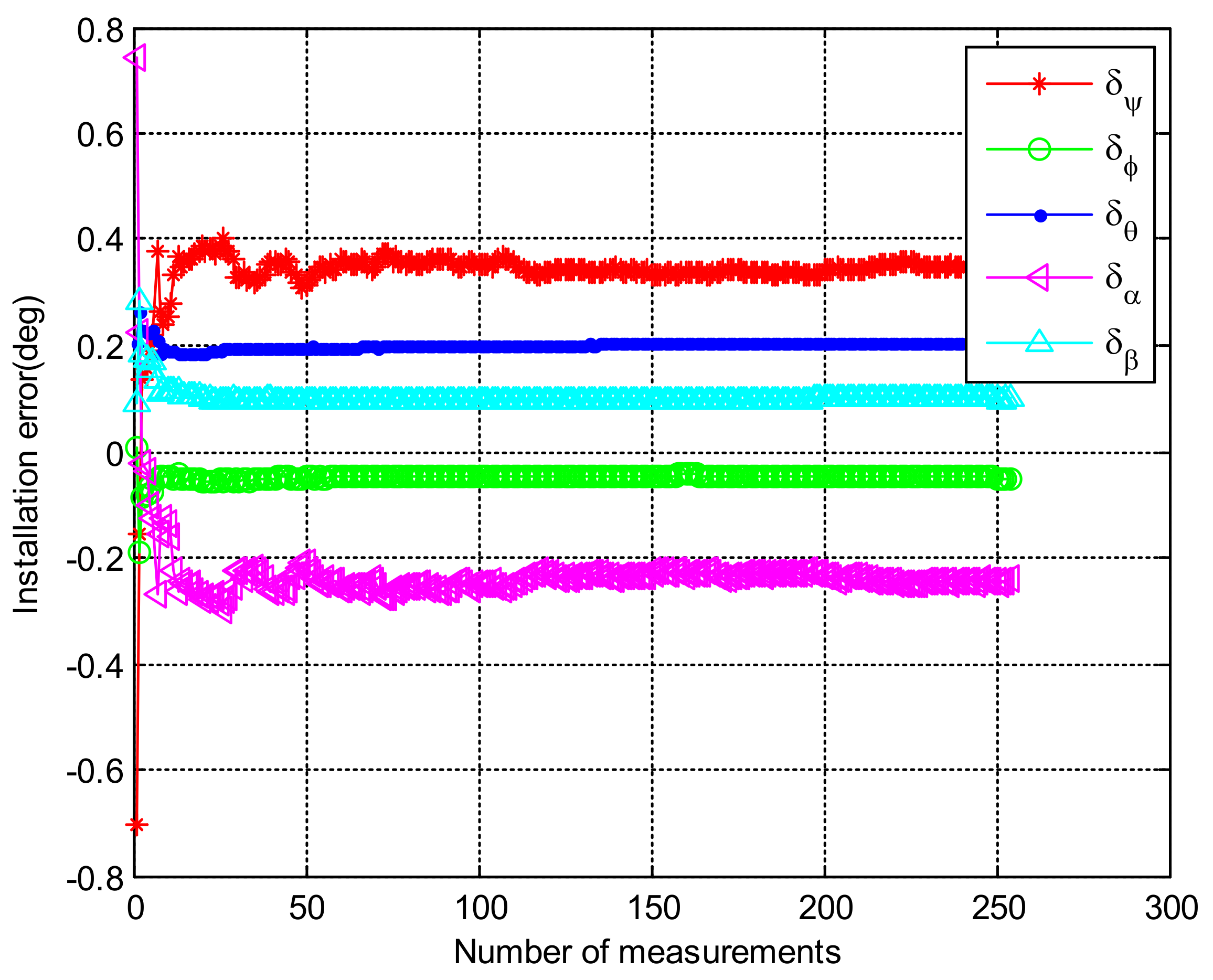
3.1.2. Systematic Error Correction and Results

Assuming that the installation error of the integrated navigation system is 0.30° for the heading direction, −0.05° for the pitch direction, and 0.20° for the roll direction, the installation error of the image coordinate frame is −0.20° for the azimuth angle and 0.10° for the pitch angle, and the control point is at (33.980849° N, 107.523239° E, 3132.10 m). In the simulation, the aircraft takes multiple imaging measurements on the control points at different positions and in different attitudes to get the installation error. The systematic error and measurement errors are shown in

Table 1. Systematic error and random measurement error in the geo-location.

Error Type	Name of Error Variable	Symbol	Error Value
Systematic error	POS installation error	Roll	0.2°
		Pitch	−0.05°
		Yaw	0.3°
	Payload installation error	Pitch	0.1°
		Azimuth	−0.2°
Random error	Platform position	Latitude	0.0001° (10 m)
		Altitude	0.00012° (10 m)
		Altitude	10 m
	Platform attitude	Roll	0.02°
		Pitch	0.02°
		Yaw	0.05°
	Payload angle	Pitch	0.027°
		Azimuth	0.027°
	Laser range	Laser	5 m

.

After performing 256 measurements on the control point, we got the installation error shown in Figure 7.

From Figure 7, it is not difficult to see that after 100 imaging measurements on the control points, the five installation errors are calculated as follows: the integrated navigation system heading direction is 0.349°, the pitch direction is −0.047°, the roll direction is 0.199°. The azimuth angle of the imaging coordinate frame is −0.244°, and the pitch angle is 0.095°. Compared with the actual installation error, the calculated errors are 0.049°, and −0.003°, 0.001°, 0.044° and −0.005°, which are only 1/6 of the original installation error. After 100 measurements, the calculated installation errors have not changed significantly. Therefore, the actual application can consider more than 100 measurements on the control points to estimate the installation error for the platform.

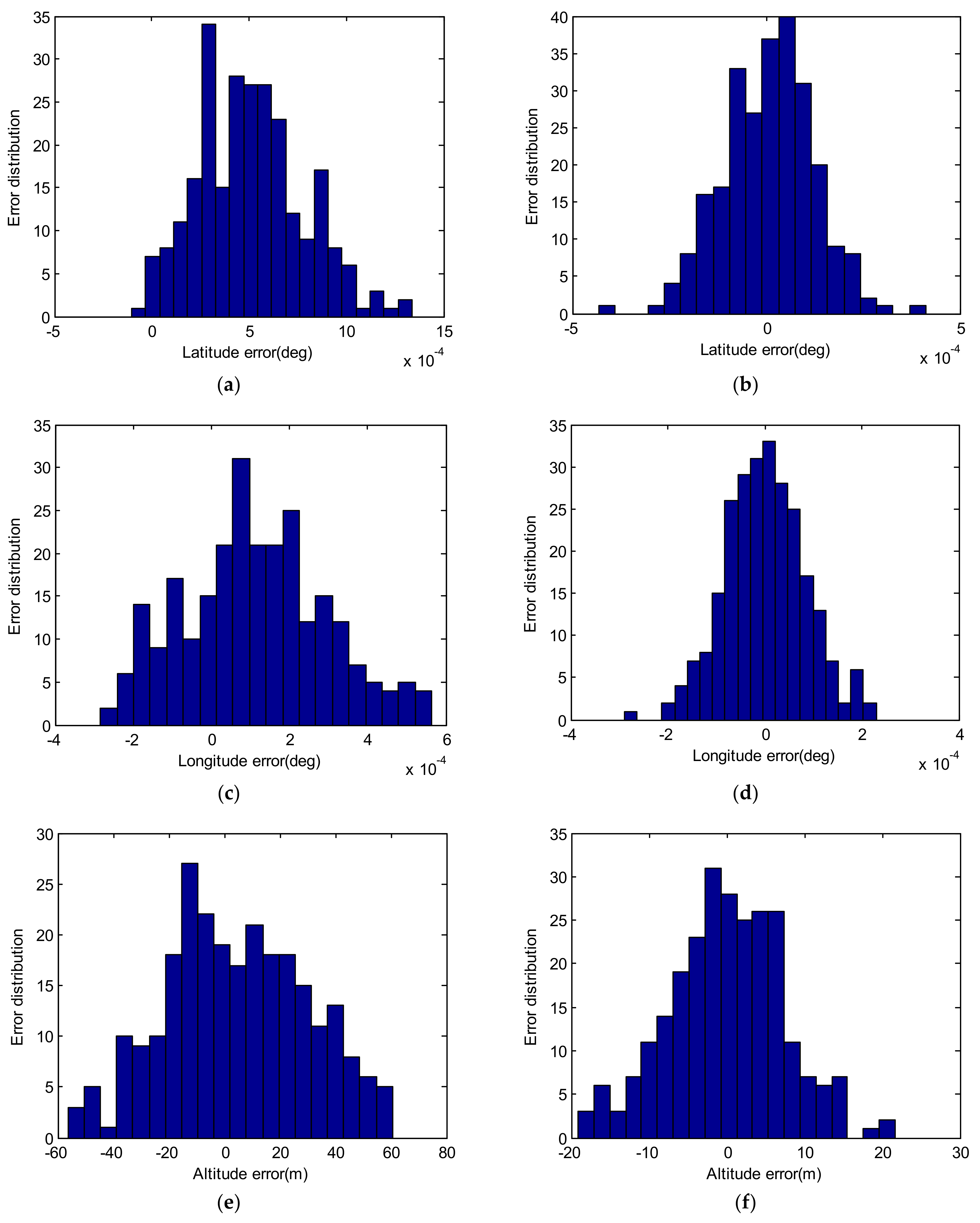
Using the measurement error and systematic error data in Table 1, using the control point and aircraft positions, the geo-location results are shown in the Figure 8a,c,e. The root mean square error of the geo-location at this time is calculated to be 53.28 m, and the mean value of the positioning error is (0.0005126°, 0.0001104°, 4.67 m) or 22.13 m. Due to the installation error, the mean error of the target positioning result is not zero.

After the installation error is corrected with the systematic error obtained above, the geo-location data is shown in Figure 8b,d,f. It is calculated that the root mean square error of the positioning at this time is 13.61 m, and the mean value of the geo-location error at this time is (0.0000076°, 0.0000011°, −0.03 m), which corresponds to 6.37 m. The comparison between before and after correction is shown in

Table 2. The comparison of geo-location between before and after correction.

Conditions	Items	Longitude (deg)	Latitude (deg)	Altitude (m)	Error (m)
before correction	sigma	0.0002730	0.0001810	25.68	53.28
	mean	0.0005126	0.0001104	4.67	22.13
after correction	sigma	0.0001165	0.0000836	7.44	13.61
	mean	0.0000076	0.0000011	−0.33	6.37

. After the systematic error were corrected, the root mean square error is reduced to 1/3 of the original, and the mean value of the geo-location error is closer to zero. The use of methods such as a Kalman filter, etc. for geo-location would be more accurate after the systematic errors were corrected.

3.2. Flight Experiments and Results

In order to verify the method mentioned above, a UAV equipped with a POS system and the airborne optoelectronic platform was used for flight experiments.

3.2.1. Design of Flight Experiments

Four target points were set as shown in

Table 3. Position of target points.

Target ID	Position (B, L, H)	Usage
P1	(124.5797389 E, 44.9517639 N, 155 m)	For errors solving
P2	(124.5818472 E, 44.9517556 N, 155 m)	For validation
P3	(124.5809611 E, 44.9523944 N, 155 m)	For validation
P4	(124.5810250 E, 44.9516056 N, 155 m)	For validation

. The targets of control points were laid on the ground, and their geographical positions were measured by a DGPS device and the geo-location error of the target <0.2 m via the post-processing, which is much less than the geo-location error analyzed in Section 3.1. Thus, the target geo-graphical position can be viewed as the source of truth.

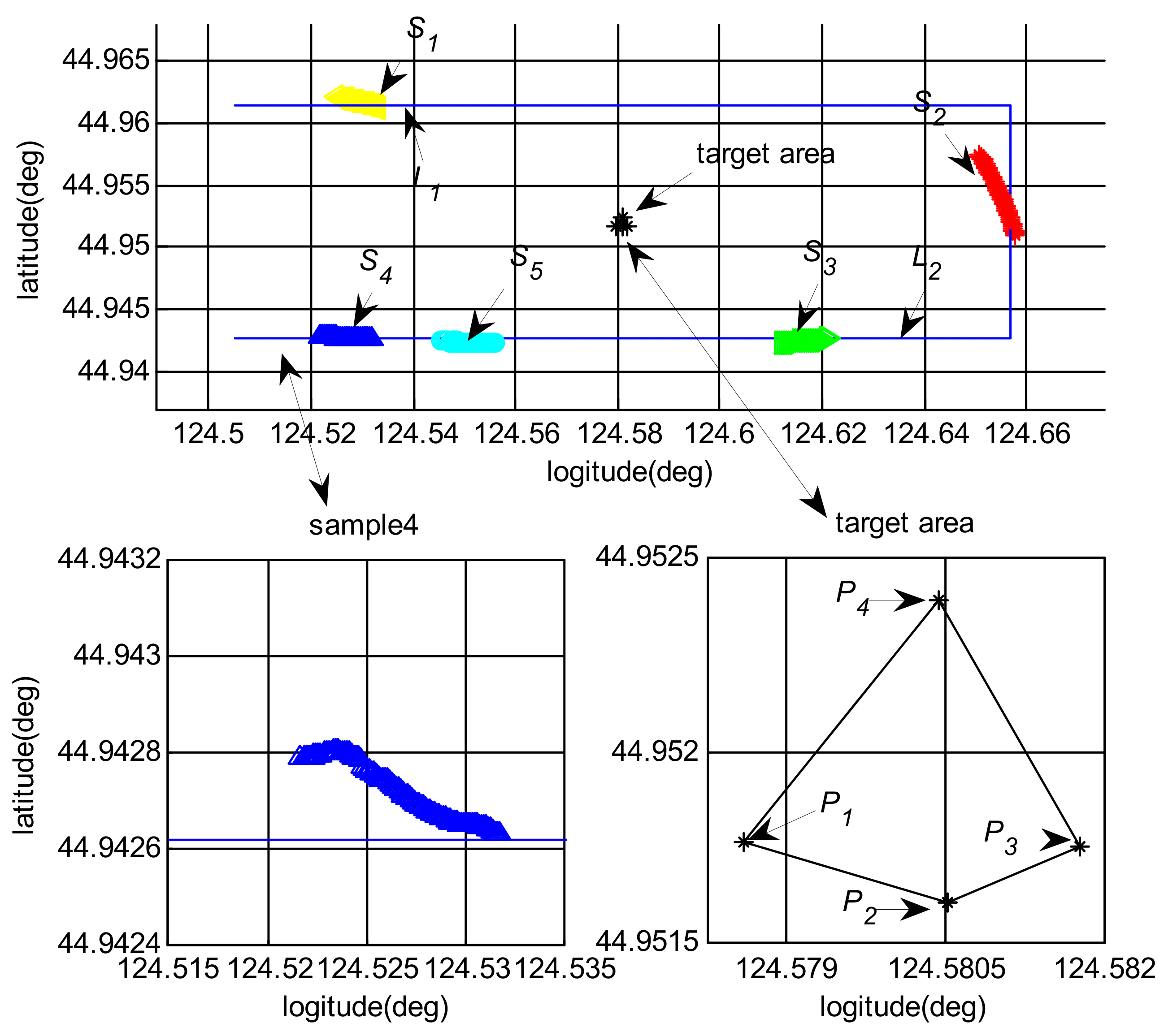
The UAV’s relative flight heights were set to 2500, 3000 and 3500 m. Five flight routes were set to achieve multiple positions and multiple angles to measure those targets as shown in

Table 4. Position of flight routes.

Route ID	Start Waypoint (B, L, H)	End Waypoint (B, L, H)
L1	(124.5152661 E, 44.9594875 N, 2500)	(124.6667839 E, 44.9594875 N, 2500)
L2	(124.5152661 E, 44.9406178 N, 3000)	(124.6667839 E, 44.9406178 N, 3000)
L3	(124.5152661 E, 44.9594875 N, 3500)	(124.6667839 E, 44.9594875 N, 3500)
L4	(124.5152661 E, 44.9406178 N, 3000)	(124.6667839 E, 44.9406178 N, 3000)
L5	(124.5152661 E, 44.9594875 N, 3000)	(124.6667839 E, 44.9594875 N, 3000)

. The routes of L1, L2 and L3 were used for the error solving and the routes of L4 and L5 were used to obtain samples for validation. The routes of L1, L3 and L5 have the same start and end waypoints with different relative flight height, and the route of L2 and L4 have the same start and end waypoints with different relative flight height too. The flight routes and target points are shown in Figure 9.

3.2.2. Systematic Error Solving

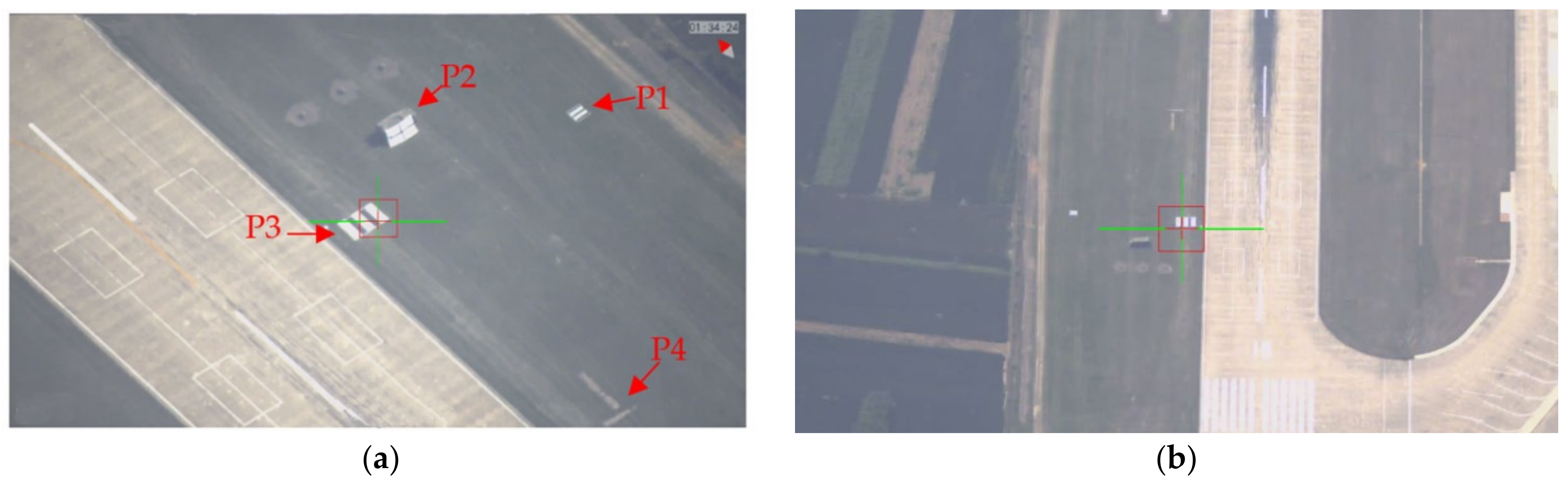
Figure 10a shows the plane flies on the left side of the target (route L1) and Figure 10b shows the plane flied along the target (route L2).

Table 5. Samples of flight routes and relevant target points.

Sample ID	Route ID	Target ID	Usage	Number of Samples
S0	L1, L2, L3	P3	For errors solving	260
S1	L5	P1	For validation	100
S2	L5	P2	For validation	100
S3	L4	P3	For validation	50
S4	L4	P4	For validation	100
S5	L5	P1	For validation	100

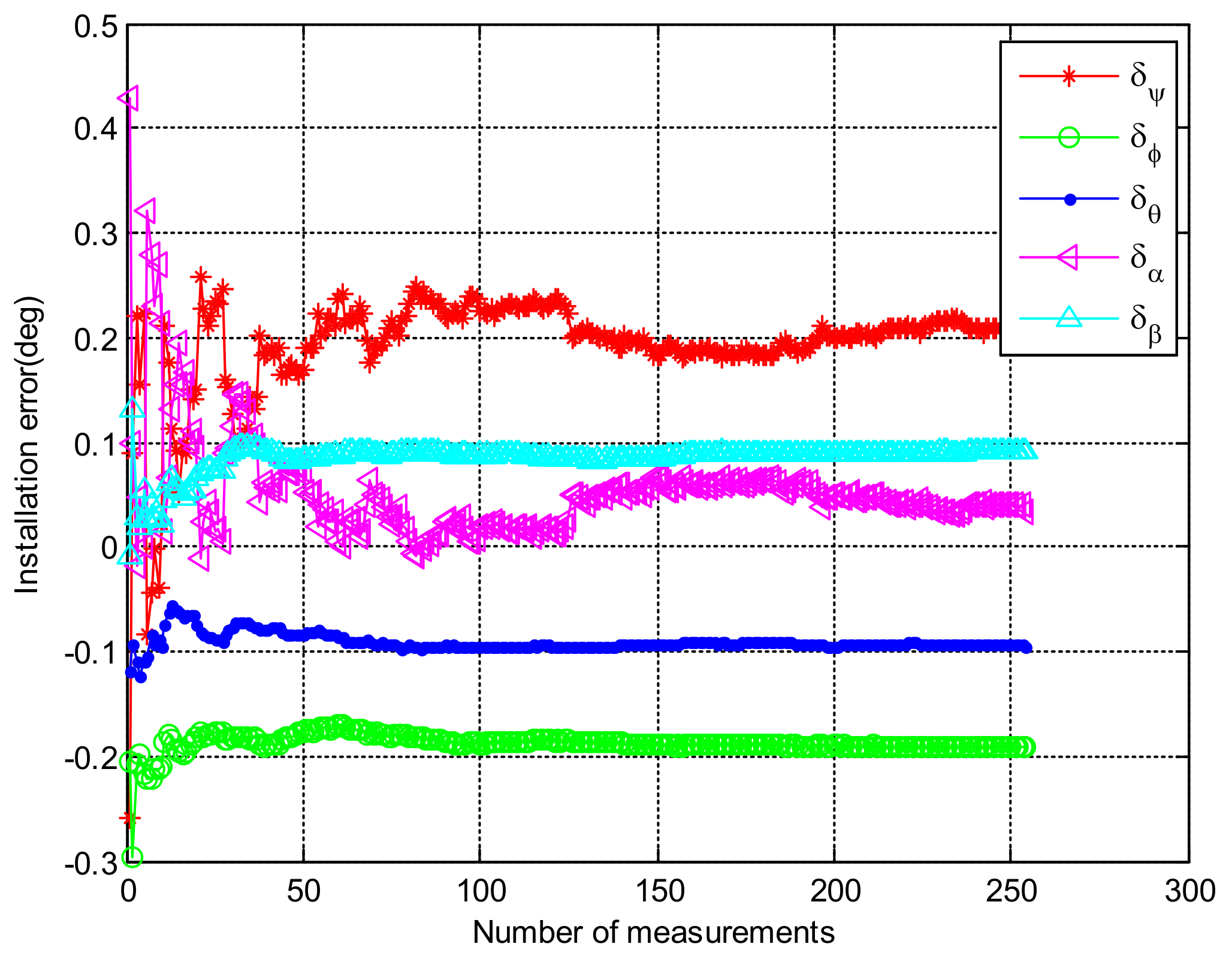
shows the Samples of flight routes and relevant target points. A total of 260 sets of measurement data were obtained. Using the method mentioned in Section 2.3, the 260 sets of data are used to solve the best estimator of the systematic error and the computation result was shown in Figure 11.

From Figure 10, it is not difficult to see that after 200 imaging measurements on the control points, the five installation errors are calculated as follows: the integrated navigation system heading direction is 0.206°, the pitch direction is −0.198°, the roll direction is −0.098°. The azimuth angle of the imaging coordinate frame is 0.061°, and the pitch angle is 0.097°.

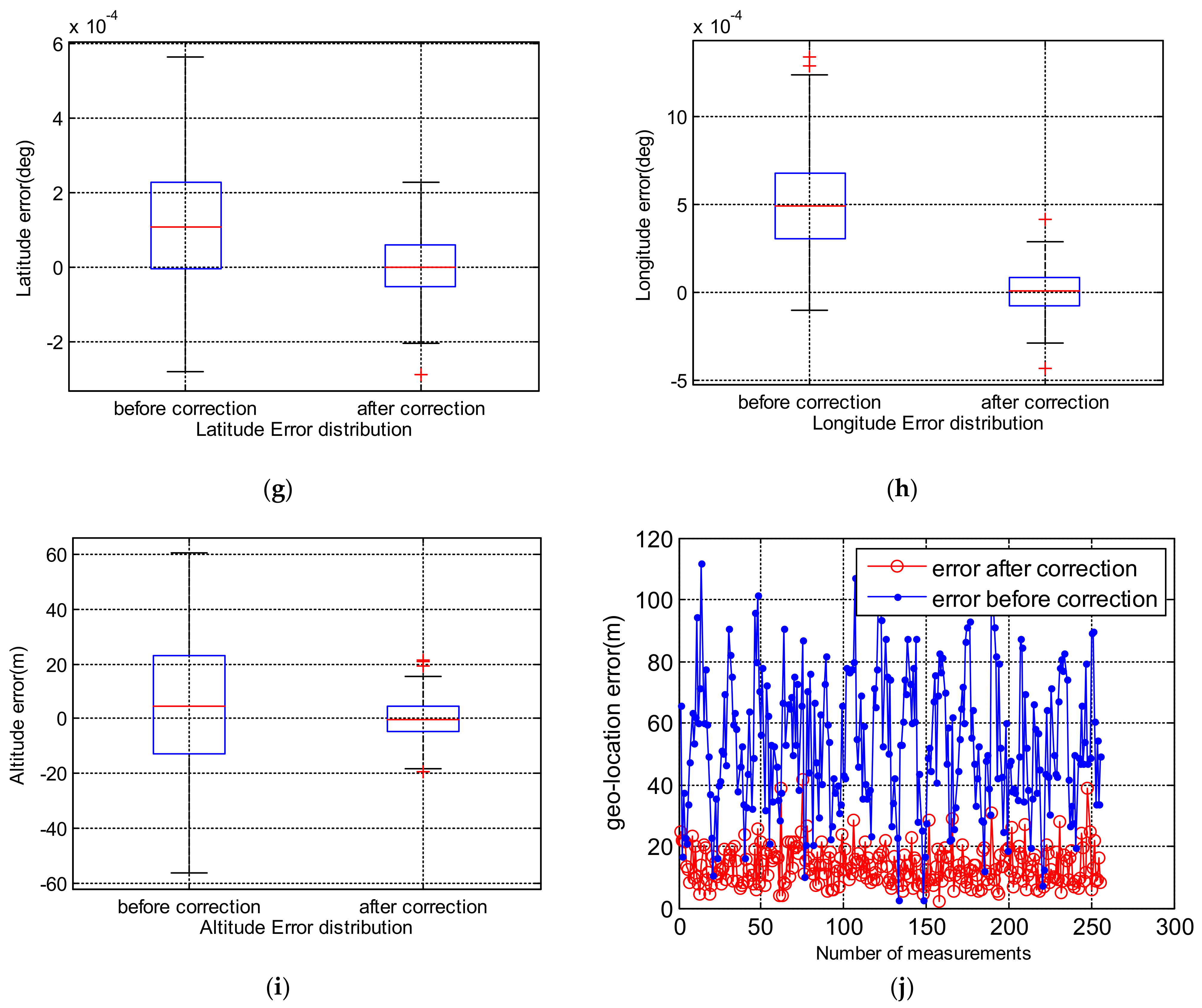
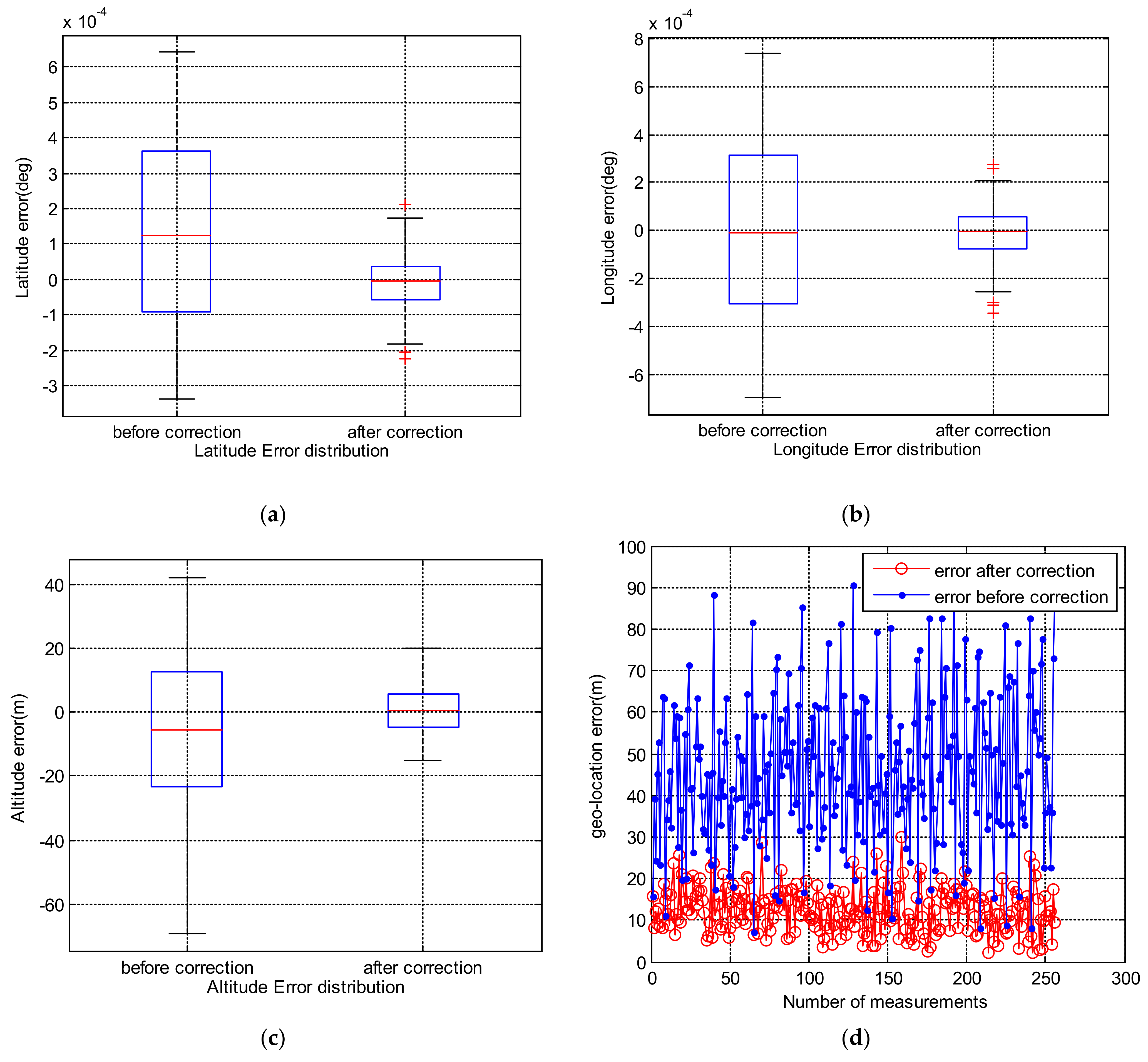
The geo-location error before and after systematic error correction of sample 0 is shown in Figure 12, where Figure 12a–c are the box plot of latitude, longitude and altitude, respectively. After correction, the root mean square error of latitude, longitude and altitude is reduced, and the mean value of the geo-location error is closer to zero.

Table 6. The comparison of geo-location between before and after correction.

Conditions	Items	Longitude (deg)	Latitude (deg)	Altitude (m)	Error (m)
before correction	sigma	0.0003453	0.0002506	25.22	45.65
	mean	0.0001412	0.0001395	−5.95	16.60
after correction	sigma	0.0001021	0.0000745	7.17	12.62
	mean	0.0000044	0.0000010	0.55	1.24

is more intuitive. The root mean square error of target positioning is reduced from 45.65 to 12.62, and the target positioning accuracy is also reduced from 16.60 m to 1.24 m. The error correction effectively improves the geo-location accuracy of the system.

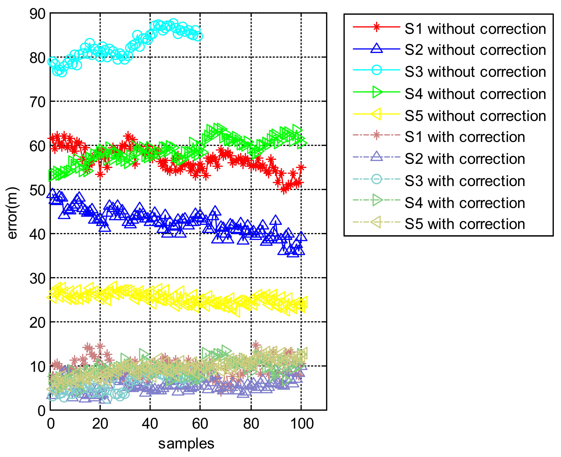
3.2.3. The Flight Experiments Validation of the Systematic Error Correction

Substituting the systematic error into the sample data for verification, we got the comparison of geo-location between before and after corrections. The geo-location accuracy of the verification data has been significantly improved. Figure 13 shows the geo-location errors of sample data S1–S5 and we can see that the geo-position error of sample data S1–S5 reduce from about 55, 45, 80 and 26 m to 10, 6, 8 and 9 m. 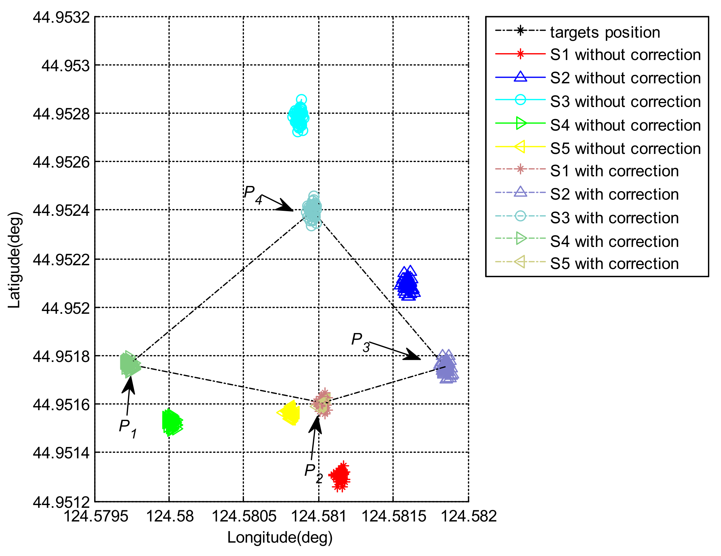Figure 14 shows a more direct view of the improvement of the accurate of geo-location. In this image, we plot the geo-location results and the target points in geodetic frame. After correction, the geo-location results were closer to the target points.

4. Discussion

From the simulation analysis and flight experiment verification above, the method proposed in this paper can effectively solve the systematic error. This error can not only reduce the root-mean-square value of the geo-location error, but also make the mean error closer to 0, making preliminary preparations for future filtering:

(1)

Selection of sample points

In order to avoid the singularity of the matrix $\left(X^{T}X\right)$ in Equation (22), samples in a variety of states should be selected, such as the aircraft at different flying heights, positions, and different attitudes. The installation error can be solved more stably. Since different platforms have different laser rangefinder, it difficult to give a suitable flight path for the calibration. But through simulation and flight experiment, it is recommended that the UAV flies on the left side and right side of the target, and take sample during the azimuth angle near 45, 135, 225 and 325 deg, respectively.

(2)

Solving the azimuth and heading angle errors

It can be seen from the systematic error iterative graph in Figure 8 that the roll angle, pitch angle installation error of the POS system and pitch angle error of the platform generally achieved stable results after about 50 measurements. However, the POS heading angle, the installation error and the azimuth angle of the platform require about 200 measurements to obtain stable values. This is because when the platform’s installation errors are small, the azimuth angle and the heading angle have the same axis, so there will be coupling when solving. The sum of the errors of the two axes will stay at a fixed value, as shown in Figure 10. Calculations show that if the sum of the two errors remains at a fixed value, the final geo-location accuracy will not be affected.

5. Conclusions

This paper proposes a systematic error correction method based on flight data. First, based on the kinematics characteristics of the airborne optoelectronic platform, the geo-location model was established. Then, the error items that affect the geo-location accuracy were analyzed. The installation error between the platform and the POS was considered, and the installation error of platform’s pitch and azimuth was introduced. After ignoring higher-order infinitesimals, the least square form of systematic error is obtained. Therefore, the systematic error can be obtained through a series of measurements. Both Monte Carlo simulation analysis and in-flight experiment results show that this method can effectively obtain the systematic error. Through correction, it can not only reduce the root-mean-square value of the geo-location error, but also make the mean error closer to 0, making preliminary preparations for filtering further.

The method proposed here mainly focuses on the systematic error correction for airborne optoelectronic platforms with laser rangefinders, which have multiple rotation axes such as azimuth and pitch axes. Through this method, we can not only get the misalignment between the platform and the body coordinate system established by the inertial instruments, but the systematic error of the rotation axis inside the platform. As for more rotation axis platforms, we just need to add more systematic error items and expand the equation. There are differences between this method and the common boresight calibration: first, this method introduces more calibration items than just misalignment between imaging coordinate system and body coordinate system with inertial instrument; second, this method applies to platforms with laser rangefinders to measure the distance between the imaging coordinate system and targets, which is different from getting boresight angles from images.

This method can be widely used in the systematic error correction and geo-location of relevant photoelectric equipment. The next step we will focus on how to filter and locate both stationary and moving targets in real time after systematic errors are corrected.