Article

Information Extraction and Named Entity Recognition Supported Social Media Sentiment Analysis during the COVID-19 Pandemic

1
Department of Information Systems, ELTE Eötvös Loránd University, 1117 Budapest, Hungary
2
Department of Informatics, J. Selye University, 945 01 Komárno, Slovakia
*
Author to whom correspondence should be addressed.
Appl. Sci. 2021, 11(22), 11017; https://doi.org/10.3390/app112211017
Submission received: 18 October 2021 / Revised: 14 November 2021 / Accepted: 17 November 2021 / Published: 20 November 2021

Abstract

:
Social media platforms are increasingly being used to communicate information, something which has only intensified during the pandemic. News portals and governments are also increasing attention to digital communications, announcements and response or reaction monitoring. Twitter, as one of the largest social networking sites, which has become even more important in the communication of information during the pandemic, provides space for a lot of different opinions and news, with many discussions as well. In this paper, we look at the sentiments of people and we use tweets to determine how people have related to COVID-19 over a given period of time. These sentiment analyses are augmented with information extraction and named entity recognition to get an even more comprehensive picture. The sentiment analysis is based on the ’Bidirectional encoder representations from transformers’ (BERT) model, which is the basic measurement model for the comparisons. We consider BERT as the baseline and compare the results with the RNN, NLTK and TextBlob sentiment analyses. The RNN results are significantly closer to the benchmark results given by BERT, both models are able to categorize all tweets without a single tweet fall into the neutral category. Then, via a deeper analysis of these results, we can get an even more concise picture of people’s emotional state in the given period of time. The data from these analyses further support the emotional categories, and provide a deeper understanding that can provide a solid starting point for other disciplines as well, such as linguistics or psychology. Thus, the sentiment analysis, supplemented with information extraction and named entity recognition analyses, can provide a supported and deeply explored picture of specific sentiment categories and user attitudes.

1. Introduction

Social media has become the number one channel of communication for people. Here, they share their thoughts and opinions on different topics, and share what articles they have read etc., shaping their narrow community with these activities.
These activities have intensified during the pandemic, and people spent more time online during lockdown and home office periods. Therefore, their news consumption has changed, and social media portals have become their primary communication channel. We cannot announce the end of the epidemic yet, but we can already say that this displacement to the online space will continue in the coming periods, both in terms of work and news consumption, communication and different forms of entertainment.
We definitely need to address these manifestations on different platforms (in this case, focusing on Twitter), and as machine learning becomes more popular and important, as does natural language processing (NLP). We need to address, analyze, and research emotions related to these platforms.
There are many options for executing sentiment analyses, from ‘human categorization’ to ‘dictionary based ’ and ‘deep learning’ methods. In the field of tools, we can choose from fully ready-to-use tools, development kits, and completely custom-developed models. One such tool is ‘TextBlob’ (https://textblob.readthedocs.io/en/dev/ accessed on 1 October 2021), which is fully ready to be integrated into any analysis—just import the library, and it is ready to use. As mentioned earlier, there are also options that allow us to create our own models, and build and train them based on our own data. ‘Using Bidirectional encoder representations from transformers’ (BERT) (https://github.com/google-research/bert accessed on 1 October 2021) for sentiment analysis is one of the most powerful tools that we can use, but we can also create a ‘Recurrent neural network’ (https://developers.google.com/machine-learning/glossary/#recurrent_neural_network accessed on 1 October 2021) (RNN) or use the ‘Natural Language Toolkit’ (https://www.nltk.org/ accessed on 1 October 2021) (NLTK) with the VADER lexicon and SentimentIntensityAnalyzer.
The main goal is to train a model to sentiment prediction by looking at correlations between words and tagging it to positive or negative sentiments.
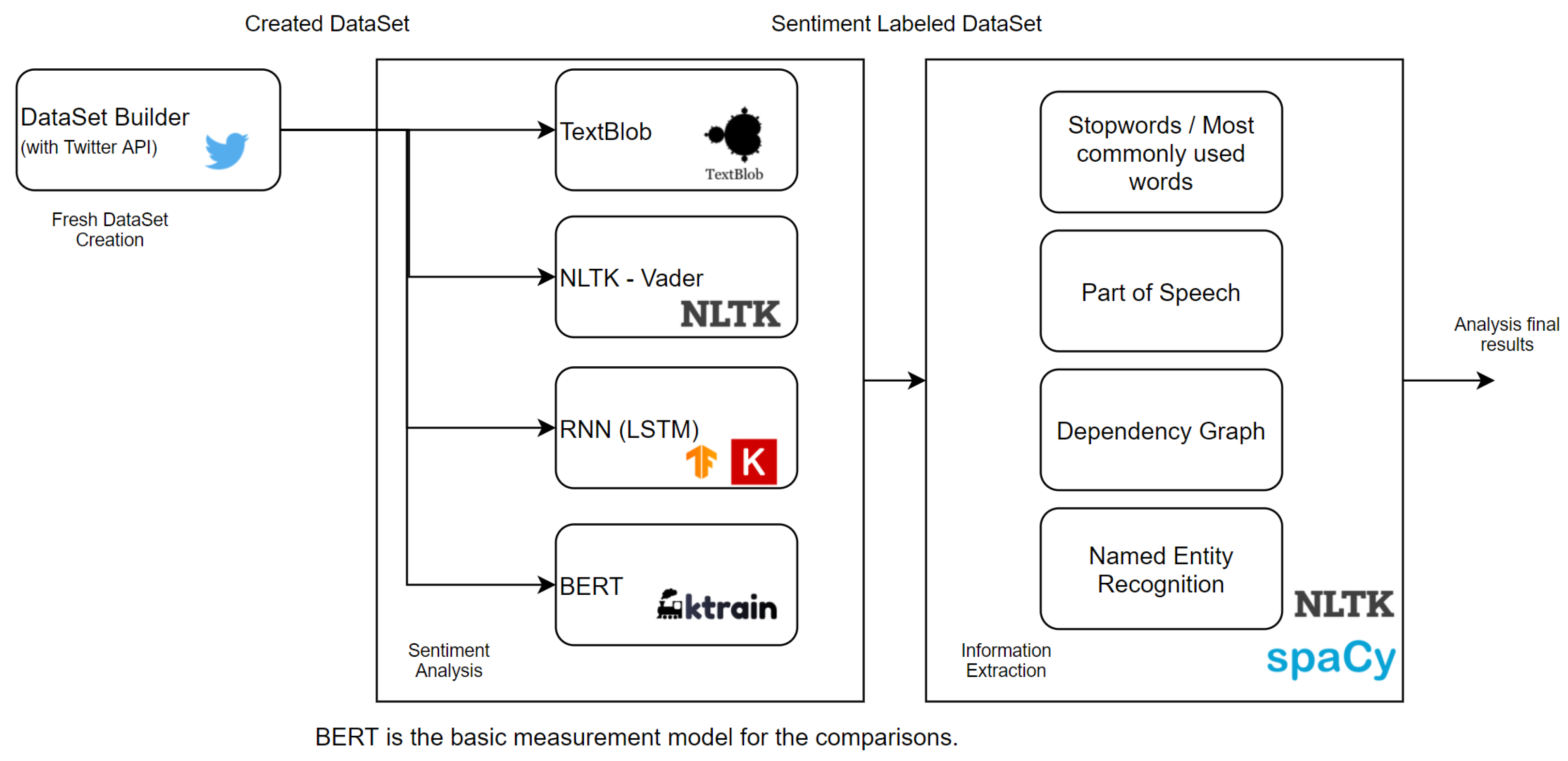
Thus, we created the RNN, BERT, NLTK–Vader lexicon models and imported the TextBlob tool into our analysis. We compared these primarily with the results of BERT. For the sentiment analyses, we also expanded the usual ‘positive’, ‘negative’, and ‘neutral’ categories with ‘strongly positive or negative’ and ‘weakly positive or negative’ options for deeper analysis, and to explore differences between models.
By performing further analysis on the data labelled by the RNN model obtained in this way, it is possible to determine, even more precisely, what emotions that the given topic evoked from people in a given time period, in the ‘COVID’ theme, in this case. For these results, we used ‘Information extraction’ (IE) and ‘Named entity recognition’ (NER) analyses.
Today is an age of information overload; the way in which we read has changed. Most of us tend to skip the entire text, whether that is an article or a book, and just read the ‘relevant’ bits of text. Journalists are also increasingly striving to highlight the most relevant information in their articles, so by only reading these highlights and headlines, we can have a ‘frame or the knowledge of the most valuable information parts’ about this subject. The task of information extraction involves extracting meaningful information from unstructured text data and presenting it in a structured format. Simplified ‘Named entity recognition’ provides a solution for understanding text and highlighting categorized data from it, where we can define different methods of the named entity recognition extraction, like ‘Lexicon approach’ or ‘Rule-based systems’, or even ‘Machine learning based system’. By performing these analyses, we can obtain deeper, information-supported sentiment results that can provide the foundation for many other research studies.
In the IE area, ‘Part of Speech’ (POS) tagging-based analyses and ‘Dependency Graph’ generation were performed, followed by NER analysis. With POS tagging, we determined which words that people use most often in positive and negative tweets, and we also examined what ‘stopwords’ occur in these cases. With the help of the ‘Dependency Graph’, we looked at what was the most positive tweet in the given analysis, and how this tweet was structured. Then, in the NER analysis, we expanded all of this, and tried to get a picture of what the differences were in the case of positive and negative tweets. What people, places, and more were mentioned in their tweets related to that topic.
The ‘spacy’ (https://spacy.io/ accessed on 1 October 2021) library provided the basics for the analyses. Like the NER analysis, it was based on default trained pipelines from ‘spacy’, which can identify a variety of named and numerical entities, including companies, locations, organizations, and products.
The RNN model was built and taught using the libraries and capabilities provided by ‘Tensorflow’ (https://www.tensorflow.org/ accessed on 1 October 2021) and ‘Keras’ (https://keras.io/ accessed on 1 October 2021). The DataSet is created and cleaned by our written scraper script, which uses the Twitter API. This script always provides the most up-to-date data, and is possible in a given time period in a given topic (COVID-19).

2. Related Works

2.1. Sentiment Analysis in Social Media

Due to the great popularity of Twitter, it can provide data for many researchers. This is similar to in [1,2], where the authors work on the scope of information exchange or triaging on Twitter in a variety of situations. This is based on the fact that different types of information are needed after different events have occurred. In terms of events, we can think of disasters or political events, and so on. This information is then classified according to credibility and then classified into primary and secondary information category. This is where the first is from the first hand and the secondary category is retweet, etc. The classification will be presented including the proposed one based on convolutional neural networks.
The authors [3] introduced a word embedding method obtained by unsupervised learning based on large twitter corpora. This method used latent contextual semantic relationships and co-occurrence statistical characteristics between words in tweets, with integration into a deep convolutional neural network.
Many people use different social media platforms as news sources, which is a significant reason to analyze them. By relying on these data, people may run the risk of drawing erroneous conclusions when reading the news or planning to purchase a product. Therefore, there is a need for systems that are able to detect and classify emotions and help users find the right information on the web. Therefore, [4], the authors propose a general approach to sentiment analysis that is able to classify the sentiments of different datasets robustly. The model is trained on the IMDb dataset and then tested on three different datasets.
There are numerous ways to measure public opinion on social platforms; users might have various degrees of influence depending on their participation in discussions on different topics. In [5], the authors combine sentiment classification and link analysis techniques for extracting stances of the public from social media (Twitter). The authors also look into the participation of popular users in social media by adjusting the weight of users to reflect their relative influence on interaction graphs, and used deep learning methods such as long short-term memory (LSTM) to learn the long-distance context.
The authors [6] proposed a novel metaheuristic method (CSK), which was based on K-means and cuckoo search. The method provides a new way to find optimal cluster heads based on the sentimental content of the Twitter dataset.
For companies, it may be worthwhile to perform sentiment analysis to assess the effects based on financial texts written by different news portals, just like foreign currency exchange rate movements [7]. In the case of English texts, this is clearly more common, and produces fairly accurate results. The authors [8] perform a similar sentiment analysis on texts provided by Lithuanian portals. They performed this analysis using two of the most commonly used traditional machine learning algorithms, naive Bayes and support vector machine (SVM), and one deep learning algorithm, long short-term memory (LSTM). Plus, they used the optimization of the hyperparameters, which was performed by grid search to find the best parameters for each classifier. The results of the applied machine learning algorithms show that the highest accuracy is obtained using a non-balanced dataset, via the multinomial naive Bayes algorithm.
In [9], the authors combined the visual content with different semantic fragments of textual content through three-level hierarchical LSTMs (H-LSTMs), to learn the inter-modal correlations between image and text at different levels. To exploit the link information effectively, the linkages among social images are modelled by a weighted relation network, and each node is embedded into a distributed vector. The authors demonstrated the effectiveness of our approach on both machine weakly labelled and manually labelled datasets.
Sentiment analysis plays/can play a significant role in improving service and product quality, and can help develop marketing and financial strategies to increase company profits and customer satisfaction. In [10], we can find out a voting classifier gradient boosted support vector machine (GBSVM), which is composed of gradient boosting and support vector machines.
Polarity detection is key for applications such as sentiment analysis. The problem with existing word embedding methods is that they often do not differentiate between synonymous, anonymous, and unrelated word pairs. In [11], the authors propose an embedding approach that solves the problem of polarity. The approach is based on embedding the word vectors in a sphere, where the point product between the vectors represents the similarity.
The sentiment analysis can be represented by the supporting vector machine. In [12], the authors propose a Fisher kernel function method based on probabilistic latent semantic analysis, which improves the kernel function of the support vector machine. With this method, latent semantic information including probabilistic characteristics can be used as classification characteristics, and to improve the effect of classification on support vector machines. The authors [13,14] gave an overview of emotion AI-driven sentiment analysis in various domains. In the considered sample data, the aspect-based ontology approach, support vector machine, and term frequency achieved high accuracy and provided better sentiment analysis results in each category. In addition, we can get to know about the ensemble learning model of sentiment classification which was presented in [15], also known as CEM (classifier ensemble model). The experiments conducted based on different real datasets found that the sentiment classification system is better than traditional machine learning techniques, such as support vector machines.
In [16], they propose a lexicon-enhanced attention network (LAN) based on text representation to improve the classification of sentiments. Combining the sentiment lexicon with attention mechanism in the word embedding module, they can obtain the sentiment-aware word embeddings as the input of the deep neural network, which bridges the gap between sentiment linguistic knowledge and deep learning methods.
Ref. [17] present a model which has become one of the most significant tools of natural language processing. BERT is designed to pretrain deep bidirectional representations from unlabelled text by jointly conditioning on both left and right context in all layers. As a result, the pre-trained BERT model can be fine-tuned with just one additional output layer to create state-of-the-art models for a wide range of tasks.
The authors [18] analyzed the public opinion related to COVID-19 in China based on social media. The number of Weibo (a Twitter-like microblogging system in China) texts has changed over time for different themes and sub-themes that correspond to different developmental stages of the event. The spatial distribution of Weibo for COVID-19 was mainly concentrated in the urban agglomerations of Wuhan, Beijing-Tianjin-Hebei, Yangtze River Delta, Pearl River Delta, and Chengdu-Chongqing. There is a synchronization between frequent daily discussions on Weibo and the trend of the COVID-19 outbreak in the real world. The reaction of the population is very sensitive to the epidemic and major social events, especially in urban agglomerations with convenient transport and large populations.

Sentiment Analysis in COVID-19

For the authors of [19], the aim of the research was to review and analyze the incidence of different types of infectious diseases, such as epidemics, pandemics, viruses or outbreaks over the last 10 years, to understand the application of sentiment analysis, and to obtain key literature findings.
In addition, by analyzing social media [20], we can learn from the 1.2 million tweets which were collected across five weeks from April–May 2021, and find out what emotions and attitudes have been evoked from people about different vaccines to COVID-19 as a response. They deploy natural language processing and sentiment analysis techniques to reveal insights about COVID-19 vaccination awareness among the public. There is a clear positive attitude of people towards vaccinations, despite the negative news that initially appeared. In addition, in the case of the security measure, people were more positive about the various topics. The authors also use TextBlob and VADER for sentiment classification.
The other huge social platform of our time is undoubtedly Instagram. In [21], the authors examined the Instagram entries of three major vaccine manufacturers. In the comments under the posts of these companies, the users’ intention to comment was mainly to make general statements, communicate facts, and share experiences, which in this context, meant their post-vaccination experience. In most cases, users do not ask for help or advice related to COVID-19 or the vaccination process. The best performing algorithms for intent classification were support vector machines and random forest, and the polarity analysis showed a highly polarized—more neutral and negative result.
Similarly, in Ref. [22], the authors applied random forest and OneR for the classification of offensive comments. Or [23], where the authors analyze the polarity of tweets with a particular vaccine and related diseases. A set of tweets were retrieved for a study about vaccines and diseases during the period 2015–2018. The results showed that the highest accuracy was achieved with the random forest model.
The authors [24] analyze the Sina Weibo popular Chinese social media site posts, where the BERT model is adopted to classify sentiment categories and the TF-IDF (term frequency-inverse document frequency) model is used to summarize the topics of posts. The analyses provide insights into the evolution of social sentiment over time, and the topic themes connected to negative sentiment on the social media sites.

2.2. Information Extraction and Named Entity Recognition

Automating clinical de-identification through deep learning techniques has been shown to be less effective in languages other than English, due to dataset scarcity. Therefore, a new Italian identification data set was created from the COVID-19 clinical records provided by the Italian Radiological Society (SIRM). Two multilingual in-depth learning systems have been developed [25] for this low-resource language scenario to investigate their ability to transfer knowledge between different languages, while maintaining the necessary features to correctly perform the Named Entity Recognition task for de-identification.
The development of COVID-19 automated detection systems based on natural language processing (NLP) techniques can be a huge help to support clinicians and detect COVID-19-related abnormalities in radiological reports. In [26], the authors propose a text classification system based on the integration of different sources of information. The system can be used to automatically predict whether or not a patient has radiological findings consistent with COVID-19, on the basis of radiological reports of chest CT. To train the text classification system, they apply machine learning approaches and named entity recognition.
The authors [27] created this CORD-NER dataset with comprehensive named entity recognition (NER) on the COVID-19 Open Research Dataset Challenge (CORD-19) corpus, which covers many new entity types related to COVID-19. CORD-NER annotation is a combination of four sources with different NER methods.
Free-text clinical notes can contain critical information to address different issues. So, we need data-driven, automatic information extraction models to use this text-encoded information in large-scale studies. Ref. [28] introduces a new clinical corpus, called the COVID-19 Annotated Clinical Text (CACT) corpus, which contains 1472 notes, with detailed notes describing the diagnosis, examination, and clinical presentation of COVID-19. The authors presented a span-based event extraction model that collectively extracts all observed phenomena and achieves high performance in identifying COVID-19 and symptom events with associated assertion values.
The huge amount of unstructured free-form text in medical records is a major barrier. An information extraction-based approach has been described by the authors [29], which automatically converts unstructured text into structured data, which is cross-referenced against eligibility criteria, using a rule-based system to determine which patients qualify for a major HFpEF clinical trial.
With X-ray images from patients with common bacterial pneumonia, confirmed COVID-19, and normal incidents, were utilized for the automatic detection of COVID-19. The aim of the authors [30] was to evaluate the performance of state-of-the-art convolutional neural network architectures proposed in recent years for medical image classification.
Besides the works discussed above, there are many other methods of sentiment analysis and data analysis. In this paper, we compare the results of sentiment analysis models, which was listed earlier (TextBlob, NLTK, RNN, BERT), and then perform further analyses on the labelled data from RNN model to explore and explain this result in more depth. Such a comparison and further analysis have not been discussed in the related works.

3. DataSet Building and Usage

3.1. Dataset Building Options

There are several possible directions for providing data for analysis, from manual work to fully automated options, or created and released data by others for free usage. These all have advantages, and possibly disadvantages.

3.1.1. Human Effort

Perhaps one of the most accurate options for creating a dataset is to collect data (tweets) on a specific topic by human effort. The probability that mismatched tweets will be included in the dataset is minimal, but of course, the human error factor still exists. This is the reason why this solution is already questionable; it is really worthwhile to create the dataset this way. This method is one of the slowest and most expensive, and is arguably an obsolete method for dataset creation. Due to the existing human error factor and cost, it is definitely worth moving in a different direction in data preparation and dataset creation.
Furthermore, our main goal is to create the fastest and most up-to-date dataset possible, where we can perform immediate analyses on up-to-date data after specific events or news.

3.1.2. Existing Datasets

You can find many pre-made and maintained datasets on the Internet. You can even think of the possibilities provided by Kaggle. In this case, we must take into account that these datasets only consist of a larger number of tweets, without any specific topics. Of course, there are also topic-specific datasets of tweets, but here, the specific topic and the given time period of the datasets cause problems.
As we wrote earlier, the goal is to use the most up-to-date datasets as possible for analysis, so that if there is any news or announcement on the topic, we can immediately run new analyses using these fresh tweets, which were written as responses to this new event on social media. Nowadays, things change very quickly, and one announcement can change a lot, and especially in the field of COVID-19, traditional polls are slow and outdated. Furthermore, when waiting for someone else to compile and publish a dataset that includes the period of time that is relevant to us, the results of the analysis may already be completely irrelevant or outdated. This is where the various scraping and api options open up to create datasets covering a given topic in a structured way as quickly as possible. This proves that we can really analyze the “average user’s” reaction and emotional attitude to certain announcements and news, and what effects that it has had.

3.1.3. Scraping and APIs

With the help of APIs provided by companies and various web scraper and helper libraries, the dataset creation can be greatly accelerated and simplified. In the case of scraping, we should definitely mention the ‘BeautifulSoup’, ‘urlopen’ and ‘Request’ libraries, which makes it easier to write dataset building scripts. In addition to these solutions, various APIs are available, such as the Twitter API, which we can use to create fresh datasets. Twitter (https://developer.twitter.com/en/docs accessed on 1 October 2021) provides an opportunity to create a dataset in this way, in a completely simple and legal way. These libraries, which we have mentioned before, can be linked to Python, but there are many other languages with similar useful libraries.
This allows us to create a fully automated fast dataset creation method, which is cost-effective, optimized for our logic, and has a minimal error factor.

3.2. Dataset Building with Twitter API

Our script (Python) only needs the given topic as a keyword, (which is ‘COVID’), a start and end date, and finally a limited number of tweets to compile a dataset on the topic that we specify. In the field of language, we use English, but this can also be changed as a parameter. The ‘tweetpy’ (https://docs.tweepy.org/en/stable/ accessed on 1 October 2021) library was used to write the script. While creating the dataset, we also perform a simple cleaning task on the dataset as well.
The dataset consists of the following values: ‘Time’—as the time, when the tweet was written, ‘UserName’—the name of the user who wrote the tweet, ‘Tweet text’—the text of the tweet, the most important data for us, ‘All Hashtags’—a list of hashtags used in the tweet and finally ‘Followers Count’—the number of followers of the user who wrote the tweet.
It is noticeable, in addition to the text of the particular tweet, that we also saved additional data, such as the follower count of the users and used hashtags. The main reason for this is, when we use information extraction after sentiment analysis, we can analyze the most positive and most negative tweets separately, which were the two most extreme opinions, and how many people were reached with these opinions, based on only the users’ follower count, without any retweet. We provide an option as a basis for further research.
Thus, it is ensured that the most up-to-date dataset is available for each analysis in a fully controlled manner. This is on the given topic, within a specified time interval, with the specified size of the dataset.

4. Methodology

4.1. Analysis Diagram

Figure 1 shows the whole process of analysis. In each case, we perform the sentiment analyses on the freshly created dataset. As mentioned earlier, BERT provides a kind of comparative result. BERT uses the transformer mechanism, which is an outstanding achievement and a remarkable breakthrough of the current NLP. Then, we continue the analyses on the dataset labeled by the “X” model, which was the closest to the BERT results. By a deeper analysis (Information extraction) of these results, we can get an even more concise picture of people’s emotional state in the given period of time.
In the course of the analyses, we do not aim to make recommendations for improvement or optimization in the case of the sentiment analysis models or the additional information extraction and named entity recognition models. We would like to present and explain our analysis and how we use/configure these models for this.

4.2. Sentiment Analysis

There are several options for performing sentiment analysis. The scale extends from labeling with human work to machine and deep learning. Natural language processing (NLP) is a very interesting topic, that can even be mentioned as a separate or unique part of artificial intelligence.
As mentioned earlier, we perform analyses on COVID-19-themed tweets from different time intervals using TextBlob, NLTK-VADER, RNN and BERT models. The results of BERT are used as a kind of benchmark against the other models. TextBlob and NLTK—VADER are third-party and easy to integrate solutions. The RNN model is our model, which we have built with ‘Tensorflow’ and ‘Keras’ frameworks. For the implementation of BERT, we used the ‘ktrain’ (https://pypi.org/project/ktrain/ accessed on 1 October 2021) library to simplify this model implementation.

4.2.1. TextBlob

TextBlob is a powerful NLP library for Python that builds on NLTK, and provides an easy-to-use interface to the NLTK library. With this tool, we can perform a variety of NLP tasks, from tagging parts of speech to sentiment analysis, and from language translation to different text classifications, but we focus on sentiment analysis. TextBlob is a lexicon-based approach, and offers two emotional metrics, polarity and subjectivity. It ignores the words that do not belong to the lexicon, and focuses only on the known words to produce a score for polarity and subjectivity measures. If we perform a sentiment analysis, we actually determine the polarity value of the sentences, where this value can be between −1 and 1. The data can be labeled with the appropriate sentiment value (positive, negative, or neutral). Here, we have expanded the given scale for a more detailed result with ‘strongly positive and negative’ and ‘weakly positive and negative’ options, and adjusted the polarity categories accordingly. If the polarity value is closer to +1, that means more ‘strongly’ positive sentiment; if this value is closer to −1, that means more or ‘strongly’ negative sentiment; 0 can be defined as a neutral sentiment on this extended slate.

4.2.2. Natural Language Toolkit (NLTK)—Valence Aware Dictionary and Sentiment Reasoner (VADER)

NLTK stands for Natural Language Toolkit. This toolkit is one of the most powerful NLP libraries which contains packages to make machines understand human language and reply to it with an appropriate response. Now, we use VADER Lexicon, and focus on sentiment analysis with the ‘SentimentIntensityAnalyzer’. VADER (Valence Aware Dictionary and Sentiment Reasoner) is a part of the Natural Language Toolkit (NLTK) packages; it is a lexicon- and rule-based sentiment analysis tool commonly used to analyze the sentiments expressed in social media, but it works well on texts from other domains as well.
VADER takes into account the polarity and intensity of emotions expressed in context, and performs particularly well when analyzing unique characters used in tweets, such as emoticons or slang. This tool produces a compound score, which scales between −1 and +1, just like in TextBlob.

4.2.3. Recurrent Neural Network (RNN)

Model

We have used tools provided by Keras and Tensorflow to build the model. We created a sequential model by passing a list of layer instances. A sequential model is appropriate for a plain stack of layers, where each layer has exactly one input tensor and one output tensor. The first layer was the embedding layer, which can be used for neural networks on text data. The embedding layer enables us to convert each word into a fixed length vector of defined size. It requires the input data to be integer-encoded, so that each word is represented by a unique integer.
Then, we used bidirectional layer (https://keras.io/api/layers/recurrent_layers/bidirectional/ accessed on 1 October 2021), which is a layer wrapper. This wrapper takes a recurrent layer as an argument. It also allows us to specify the merge mode, which is how the forward and backward outputs should be combined before being passed onto the next layer. The default mode is to concatenate, and this is the method often used in studies of bidirectional LSTMs. We used the default mode. We used LSTM layers with the bidirectional layers. The long short-term memory (LSTM) is an RNN ’architecture’; these networks constitute a type of recurrent neural network, and are capable of learning order dependence in sequence prediction problems.
Next are the dense and dropout layers. A dense layer is a classic fully connected neural network layer, and each input node is connected to each output node. A dropout layer is similar, except that when the layer is used, the activations are set to zero for some random nodes. This is a way to prevent overfitting. We used a dense layer with ‘relu’ activation, then a dropout layer, and again a dense layer with ’sigmoid’ activation.

Difference between RNN and LSTM

All RNN has a feedback loop in the recurrent layer. This allows them to maintain information in “memory” over time. However, it can be difficult to train standard RNNs to solve problems that require learning long-term temporal dependencies. This is because the gradient of the loss function decays exponentially over time; this is called the disappearing gradient problem. LSTM networks are a type of RNN that use special units in addition to standard units. LSTM units contain a “memory cell” that can maintain information in memory for a long time. A set of gates is used to control when information is written into memory, when it is output, and when it is forgotten. This architecture allows them to learn longer-term dependencies.

Trained Model Information

The RNN model was trained based on an IMDB review dataset (https://www.tensorflow.org/datasets/catalog/imdb_reviews accessed on 1 October 2021). The dataset comes from the official tensorflow catalog, which provides 25,000 highly polar reviews for training, and 25,000 for testing. We used the “subwords8k” option with a vocab size of 8185. The data consist of labels and texts. In the test and train dataset sections, we used the shuffle method as well.
The accuracy of our model was 84.7% on the test dataset. The model is not overfitting, and it is more generalized and can make good predictions for new data. Furthermore, we can mention that the buffer size was 10,000, and the batch size was 64. In the ‘compile’, the loss argument was “binary crossentropy” with the “Adam” optimizer.
We also save our trained models in ‘.h5’ format. This previously mentioned model was used to analyze further tweets.
The ‘positive’, ‘neutral’, ‘negative’ labels were expanded in this case as well, just like in the previous models with ‘strongly positive and negative’ and with ‘weakly positive and negative’ labels. Furthermore, it should be mentioned, unlike the previous models, the sentiment value (predicted compound value) here scales between 0 and +1, instead of −1 and +1 values.

4.2.4. Bidirectional Encoder Representations from Transformers (BERT)

Unlike traditional NLP models, which follow a one-way approach, i.e., reading the text from left to right or right to left, BERT reads the entire word sequence at once. BERT makes use of a transformer, which is essentially a mechanism for building relationships between words in a dataset. In a simplest form, BERT consists of two processing models—an encoder and a decoder. The encoder reads the input text and the decoder generates the predictions. However, since the main purpose of BERT is to create a pre-trained model, the encoder takes precedence over the decoder. BERT is a remarkable breakthrough in NLP.
As we have mentioned earlier, the BERT model was implemented with the capabilities provided by the ‘ktrain’ library, which is a lightweight wrapper for Tensorflow and Keras. The full concept of BERT was developed and published by Google, which has made significant progress in many areas of NLP. The significant development of Google Translate can be attributed to this as well.

Model

In the case of BERT, the model was created using the ktrain “text .text classifier” method and then the “get learner” method. The “get learner” parameter received the “text .text classifier”, train and validation data and the batch size, which was 6.
About the data: 25,000 labeled reviews were used as a train dataset, and 25,000 labeled reviews were used as a validation dataset for the model, where the text column was ‘Reviews’, and the label column was ‘Sentiment’.
The training was done with the help of the “fit onecycle” method, where the value of the learning rate parameter was “2 × 10 5 ” (lr = 2 × 10 5 ).

4.3. Information Extraction

Information extraction is the process of extracting information from unstructured textual sources to enable finding entities and classifying or storing them in a database, or preparing this information for further analysis, so that the task of information extraction (IE) is to extract meaningful information from unstructured textual data and present it in a structured form.
In general, extracting structured information from unstructured texts involves the following main subtasks:
  • Pre-processing of the text—where the text is prepared for processing with the help of computational linguistics tools such as tokenization, sentence splitting, morphological analysis, etc.
  • Finding and classifying concepts—where mentions of people, things, locations, events and other predefined concepts are perceived and classified.
  • Connecting the concepts—the task of identifying relationships between the extracted concepts.
  • Unifying—this task is presenting the extracted data into a standard form.

4.3.1. Part of Speech (POS)

We all know that sentences consist of words belonging to different parts of speech (POS). Some of these POS are: noun, pronoun, verb, adjective, adverb, preposition, conjunction, and intersection.
POS determines how a particular word works in the meaning of a particular sentence. For example, the word ‘right’. In the sentence, “The boy was awarded chocolate for giving the right answer”, ‘right’ is used as an adjective. Meanwhile, in the sentence, “You have the right to say what you want,” ‘right’ is treated as a noun.
POS tag of a word carries a lot of significance when it comes to understanding the meaning of a sentence. However, sometimes extracting information purely based on the POS tags is not enough. If we would like to extract the subject and object from a sentence, we cannot do that based on POS tags. For that, we need to look at how these words are related to each other.
There are several methods of the POS, such as the ‘Rule-Based POS tagging’ method, which uses contextual information to assign tags to unknown. For example, if an ambiguous/unknown word X is preceded by a determiner and followed by a noun, it will be tagged as an adjective. Meanwhile, there is ‘Transformation-based tagging’, where the tagger is based on transformations or rules, and which learns by detecting errors. On the other hand, ‘Stochastic (Probabilistic) tagging’ is based on the probability of a certain tag occurring.
We used the methods of the ‘spacy’ and ‘nltk’ libraries to perform the analyses. The choice of ‘spacy’ was conscious, to use a library which is a popular choice in the industry as well, in addition to the scientific approach.
Spacy can make predictions about which tag or label most likely applies in this context, which is based on the trained pipeline and its statistical models. A trained component includes binary data that are produced by showing a system enough examples for it to make predictions that generalize across the language.

4.3.2. Dependency Graph

Dependency parsing is the process of analyzing the grammatical structure of a sentence and finding out the related words and the type of relationship between them.
Again, we used the tools provided by ‘spacy’ library. Spacy has a syntactic dependency parser. The parser powers the sentence boundary detection, and lets us iterate over base noun phrases, or “chunks”.

4.3.3. Named Entity Recognition

Named entity recognition (NER) is an information extraction task, which identifies mentions of various named entities in unstructured text, and classifies them into predetermined categories, such as people’s names, organizations, locations, date/time, monetary values, and so on.
Terms that represent specific entities are more informative and have unique contexts. Furthermore, they represent real world objects, like people, places, organizations, etc., which are often proper names. Thus, NER is a prominent factor in information extraction that identifies named entities and segmenting them into appropriate classes.
Based on this, we can define the task of NER in these three steps: Detect a named entity, extract the entity, and categorize the entity.
In the case of NER, several implementations can be used. ‘Lexicon approach’ relies on a knowledge base called ontology, and contains all terms related to a particular topic, grouped in different categories. The system looks for matches with named entities. ‘Rule-based systems’ are a series of grammatical rules hand-crafted by computational linguists. We can gain results of high precision, but low recall. Last but not least, ‘Machine learning based systems’ build an entity extractor and feed the model with a large volume of annotated training data. Here, we need tagged and clean training data.
For named entity recognition, we used ‘spacy’ library and ‘displacy’ visualizer.

5. Sentiment Analysis Results

The analyses were run in late August and early September. Accordingly, we defined time intervals (29 August 2021 and 31 August 2021, 2 September 2021 and 4 September 2021), and defined the topic keyword, which was ‘COVID’, and set the dataset size to 500 tweets to build the datasets of 500 tweets from both September and August time intervals, using the Twitter API Standard option.
We would like to present the methods of this analysis flow in the first place; we expect similar results with a larger amount of data as well. The reason for this period is that it is the period of starting school in many countries. School may have already started, or will start soon. It is a particularly important period in the knowledge of the next, fourth wave of COVID-19.

5.1. Prolog

The classification of the tweets was based on the polarity and compound values, which were obtained from the different models. The models were used here as described in the methodology section. In the case of TextBlob and NLTK-VADER, the appropriate methods of the library were parameterized and used; in the case of RNN and BERT, it was taught and used according to their previous descriptions.
The basic result is determined using the BERT transformer mechanism. We do not aim to compare all models with all other models; we would like to present and explain the methodological differences of the TextBlob, NLTK-VADER and RNN models, and then analyze the results of the model that best approached the results of BERT in more depth.
We expect the results of the RNN to be the closest to the results provided by BERT, due to its methodological sophistication.
The interval for each category was properly defined, including the extended (‘strongly’, ‘weakly’) categories as well. Based on the values, the tweets were categorized and labeled in the appropriate category. In the case of BERT, the positive and negative categories were not further subdivided, due to the role.

5.2. TextBlob

In 
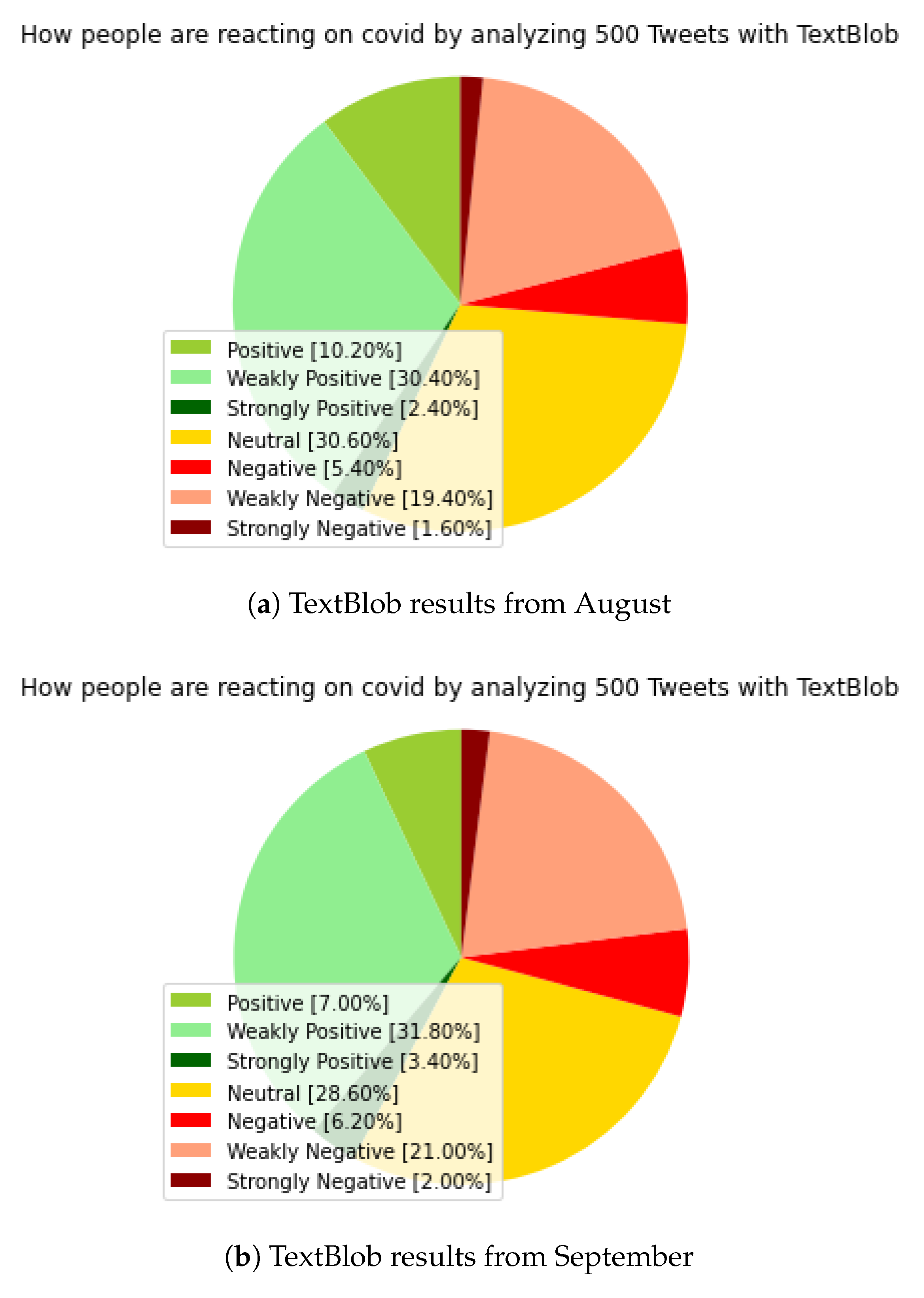
Figure 2, the neutral value dominates in both examined periods, which significantly distorts the result. The August results in Figure 2a show a 30.60 percent neutral value, which is significant. The results from September in Figure 2b also show that the neutral value is 28.60 percent. A small shift can be seen in the case of the neutral values of the two studied periods, which was in a negative direction.
In both August and September, ‘weakly positive’ values dominated their category, with 30.40 and 31.80 percentages. In the negative section, we can see a similar ‘weakly negative’ dominance. Due to the significant neutral values, the results are not exactly the most favorable for further analysis.

5.3. Natural Language Toolkit (NLTK)—Valence Aware Dictionary and Sentiment Reasoner (VADER)
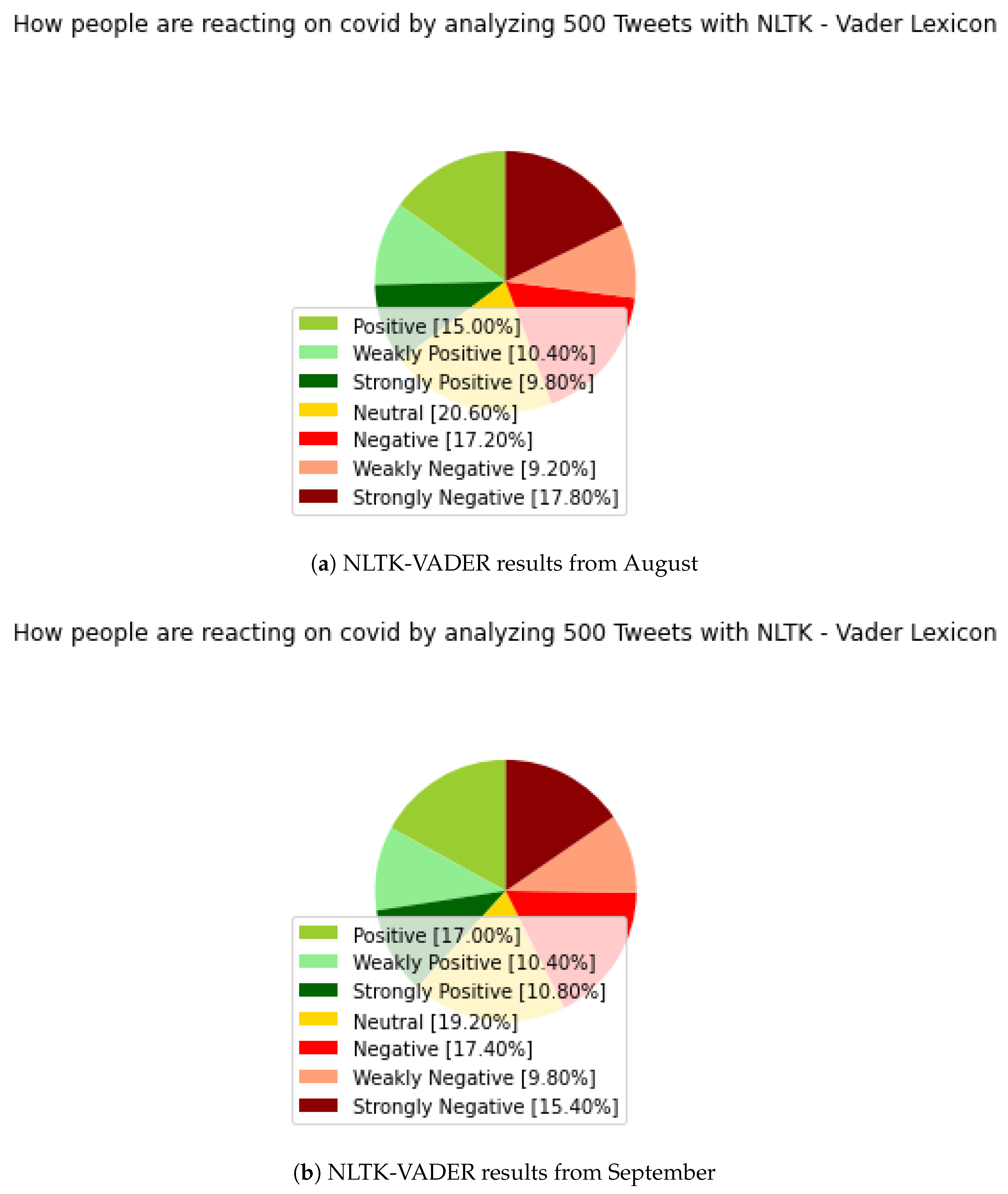
In Figure 3, the results of NLTK—VADER show a significant improvement over the results of the previous TextBlob. It is enough to look only at the values of the neutral categories and see significant differences in the stages of the positive and negative parts.
In the case of the August result, which can be seen in Figure 3a, the neutral value decreased significantly, and now it is only 20.60 percent. Similarly, in Figure 3b, the neutral value is 19.20 percent, compared to previous results, which reached 30 percent, or it was very close to this value.
In the case of the August results, there are also significant differences within the positive parts, and there is no longer such a ‘weakly positive’ dominance; due to the technological changes, we can assume a more accurate result on the same datasets as we used in the case of TextBlob. Here, we can see 15 percent ‘positive’, 10.40 percent ‘weakly positive’ and 9.80 percent ‘strongly positive’ sentiment values. In September, 17 percent ‘positive’, 10.40 percent ‘weakly positive’ and 10.80 percent ’strongly positive’ sentiment values were observed.
Similar movements can be observed in the negative sections, with 9.2 percent ‘weakly negative’, 17.2 percent ‘negative’ and 17.8 percent ‘strongly negative’ in August. In September, 9.8 percent were ‘weakly negative’, 17.4 percent were ‘negative’, and 15.4 percent were ‘strongly negative’ sentiment values. Despite a significant decrease in the neutral section, there are still too much data in this category, although we can definitely report an improvement on previous TextBlob results. The goal is to eliminate or considerably minimize the neutral values, in order to confirm the results with subsequent analyses. A neutral value still makes the result a little bit uncertain.

5.4. Recurrent Neural Network (RNN)
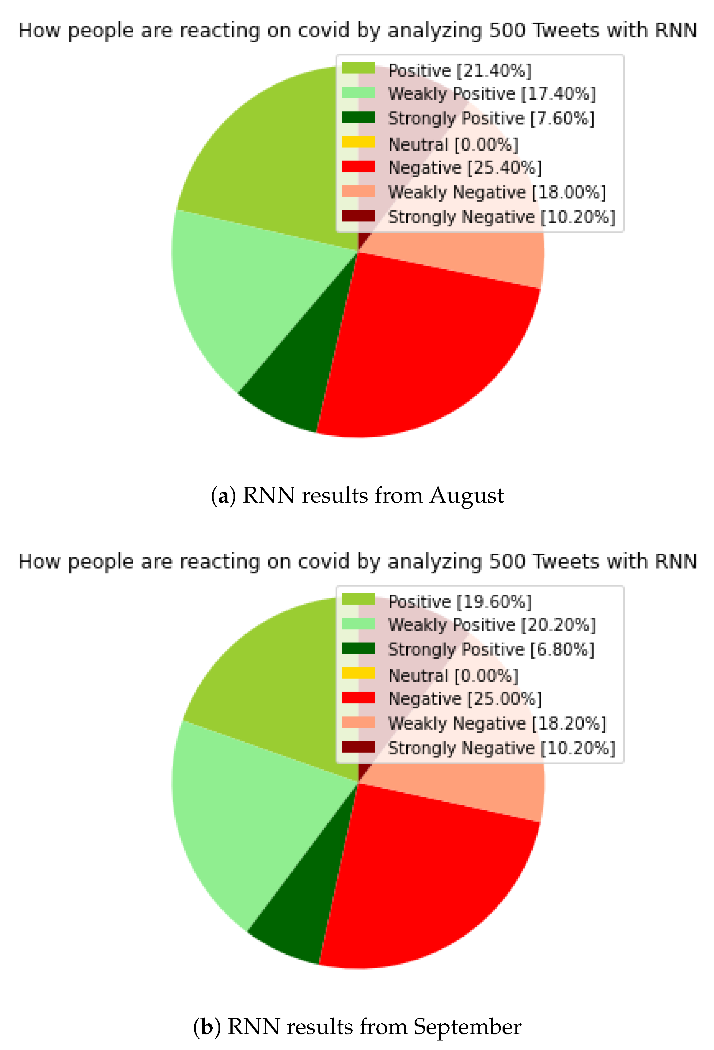
In Figure 4, the results of RNN, when compared to the previous two (TextBlob and NLTK-VADER), has a neutral section of 0 percent in both August and September results, which is a significant improvement. In addition, small changes in distribution were observed in both the positive and negative sections compared to the previous models. In the case of the previous models, especially in the case of the NLTK-VADER results, there is a similarity in the result categories, both in positive and negative sections, the huge difference, and of course the neutral category. Our model was able to place all tweets in a category, as we expected, which significantly increases the establishment of a clearer picture of these specific periods.
The value of ‘strongly positive’ was 7.60 percent in August, down from 6.80 percent in September. The ‘positive’ section was 21.40 percent in August, but it was 19.60 percent in September; the ‘weakly positive’ values rising from 17.40 percent in August to 20.20 percent in September. Overall, in addition to the changes in ratios, the positive section increased by 0.2 percent overall, but there was a shift toward the ‘weakly positive’ section.
For the negative sections, the ‘strongly negative’ value was unchanged at 10.20 percent in both August and September. The ‘negative’ value fell from 25.4 percent in August to 25 percent in September. The ‘weakly negative’ value rose from 18 percent in August to 18.2 percent. Despite a small 0.2 percentage increase in positive values, and even in the case of minimal movements inside of the negative section, the negative sections still represent a larger overall section, plus in the case of positive values, a shift toward a ‘weakly’ value should be highlighted.
In summary, the results of the RNN model and the results of previous models show a strong division; there is some kind of “boundary line” based on the studied periods, which is very difficult to move. People have their own opinions about the pandemic, which has lasted for almost two years. Due to the significant neutral result seen in the TextBlob result, it is difficult to write a conclusion, but the results of the subsequent NLTK-VADER and then the RNN results, where the neutral values decreased significantly and then disappeared, already give some picture. They show a shift in the negative direction; during the period under review, the negative sections provided a higher percentage value overall, and in the case of the RNN model, the shift to the already mentioned ‘weakly positive’ section can be highlighted again.
Vaccinations, and the relatively ‘free summer’, also provide a basis for the positive parts in the studies, and the uncertainties of starting school and the fourth wave continue to maintain a more negative attitude.

5.5. Bidirectional Encoder Representations from Transformers (BERT)

As we mentioned earlier, BERT was used as a kind of comparative result. 
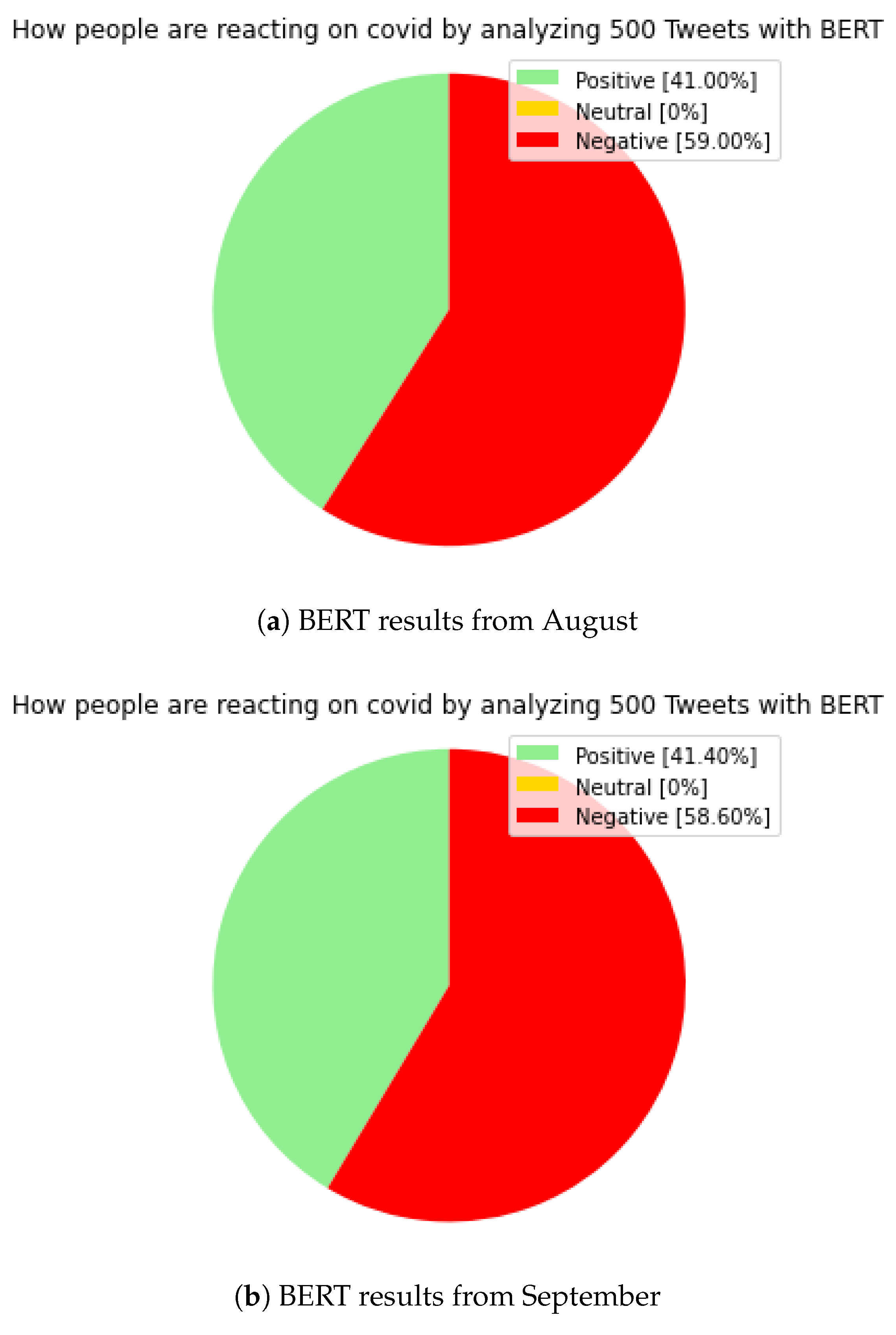
Figure 5 shows the results obtained by BERT. Of course, without the neutral category, in the case of BERT, in contrast to the previously presented models, we did not further categorize the positive and negative categories, because we only consider the results of BERT as a benchmark/comparative result for comparison to the other models, so we obtained a classic, ‘positive’, ‘neutral’, ‘negative’ result in the same time periods as in the previous models.
For the BERT model, the ‘positive’ section was 41 percent in August, which increased to 41.40 percent in September. The ‘neutral’ section was 0 percent according to our expectations. The ‘negative’ section was 59 percent in August, down from 58.60 percent in September. The results of BERT are mostly approximated by the results of the RNN model, which met our expectations.
The aggregated positive result for RNN in August was 46.40 percent, and the negative result was 53.60 percent. Similarly, in September, the aggregated positive score was 46.60 percent, and the negative was 53.40 percent. Here, we can see a slight shift in the positive direction too, but overall, the negative section dominates. This confirms the effectiveness of our RNN model, where we could also see a more detailed statement by further categorizing in positive and negative sections.
Based on the comparative results by BERT, we will perform further analyses on the results of the RNN model, to gain more insight into the sentiment results in this period. To do this, we perform information extraction (IE) and named entity recognition (NER) analyses. For the TextBlob and NLTK models, due to the significant neutral categories, we did not include a comparison with the results of BERT.
Our goal, with the help of these analyses, is to give a comprehensive picture of these periods, what sentiment states people are in, and what characterizes the tweets, which was written at that time. How the tweets were structured, what was mostly mentioned in them, and what can be said about these tweets are all important.

6. Information Extraction Results

As we have mentioned earlier, these analyses are performed on the results of the RNN model. After the sentiment analyses, we have aggregated the extended sentiment categories, so the analyses were performed on separate positive and negative datasets.

6.1. Prolog

We started the POS analysis by comparing the ‘stopwords’ (which words occur in a positive and negative attitude), and then, we followed this with the most commonly used words in the same categorization approach. The “nltk.corpus” (‘stopwords’ download and inclusion in the analysis) and “nltk.tokenize” libraries were used.
This was followed by the ‘stopwords’ removals and re-tokenization of tweets, with the entire POS analysis, which covers the positive and then the negative category. Finally, for the most followed positive tweets, we built dependency graphs. The ‘spacy’, ‘spacy—en core web sm’ pipeline and the ‘displacy’ visualization option were used for these analyses.

6.2. Stopwords and Most Commonly Used Words

Stopwords are the most common words in any natural language. For the purpose of analyzing text data and building NLP models, these stopwords might not add much value to the meaning of the document.

6.2.1. August

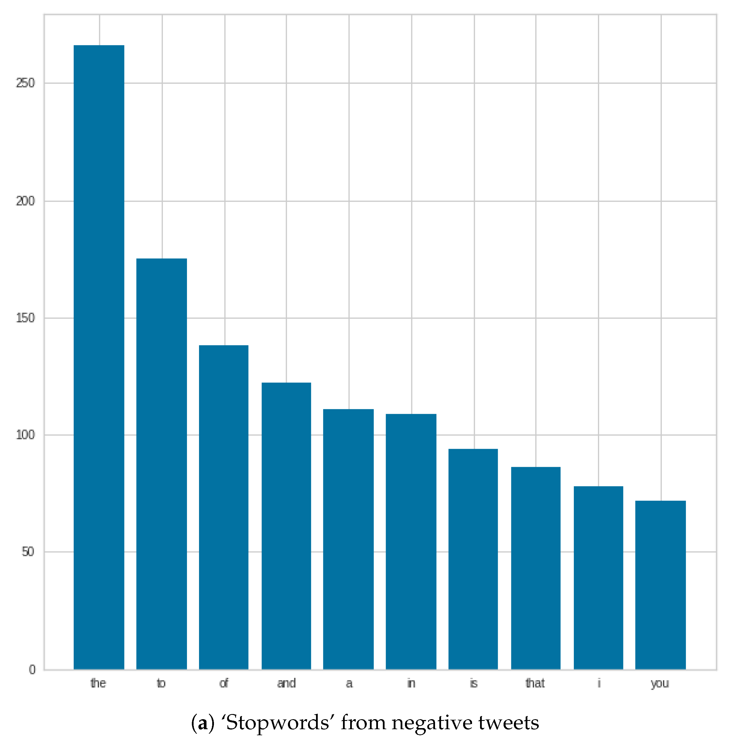
Figure 6 shows that ‘stopwords’ were very similar in both positive and negative tweets, and in some cases, we see changes in positions, such as ‘and and ’of’. In addition, in the negative case, the number of ‘the’s can be highlighted.
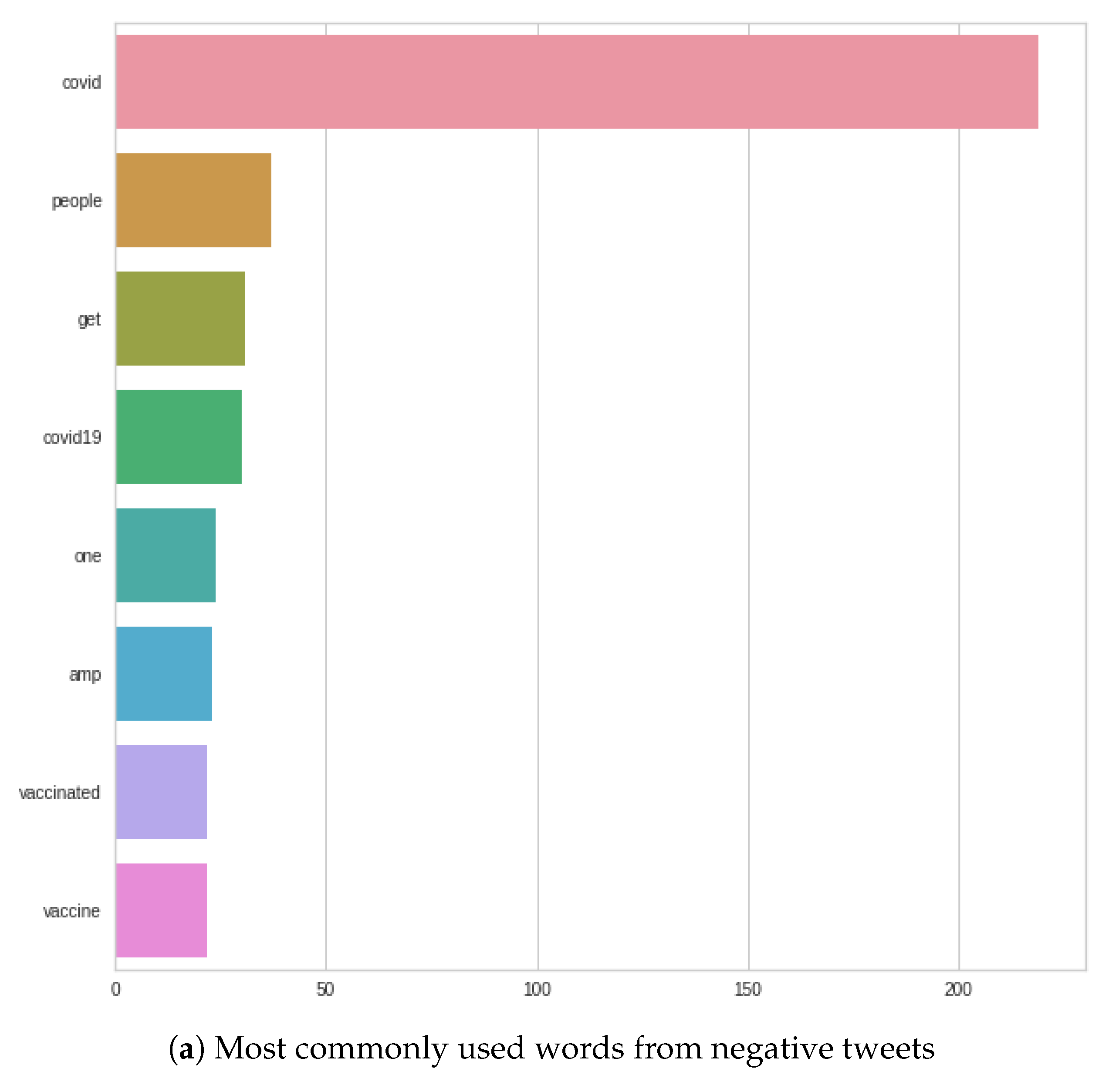
Figure 7 shows that, for the most commonly used words, the word ‘COVID’ completely dominates in both negative and positive tweets. After that, there are differences, such as in the negative case, where the word ‘COVID’ is followed by the following words: ‘people’, ‘get’, ‘COVID-19’; as opposed to the positive case, where the next three words are: ‘COVID-19’, ‘people’, ‘vaccine’. In the negative case, ‘vaccine’ or ‘vaccinated’ appear only at the very end of the figure, in contrast to positive tweets, where ‘vaccine’ is the fourth most common word.

6.2.2. September

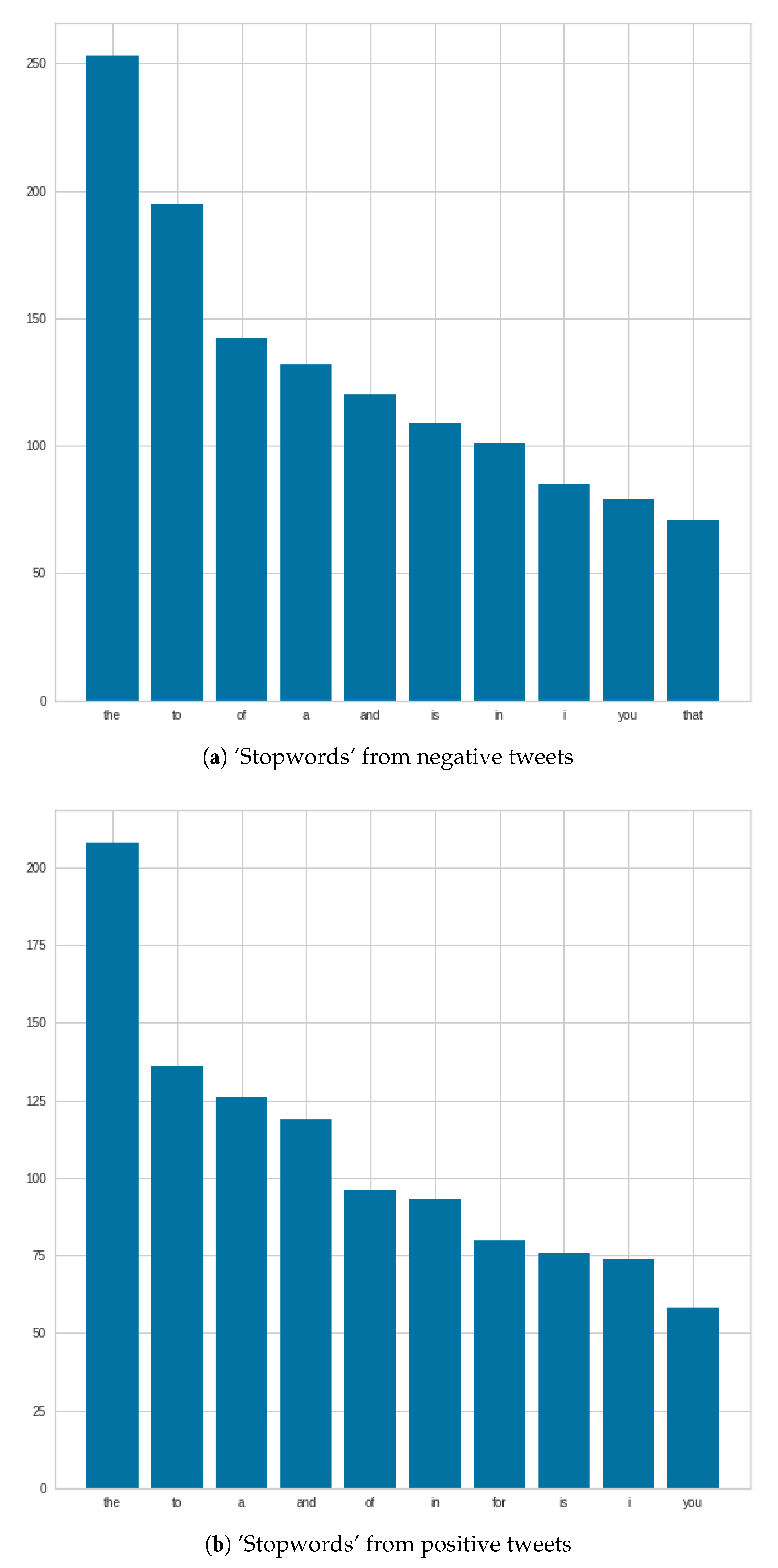
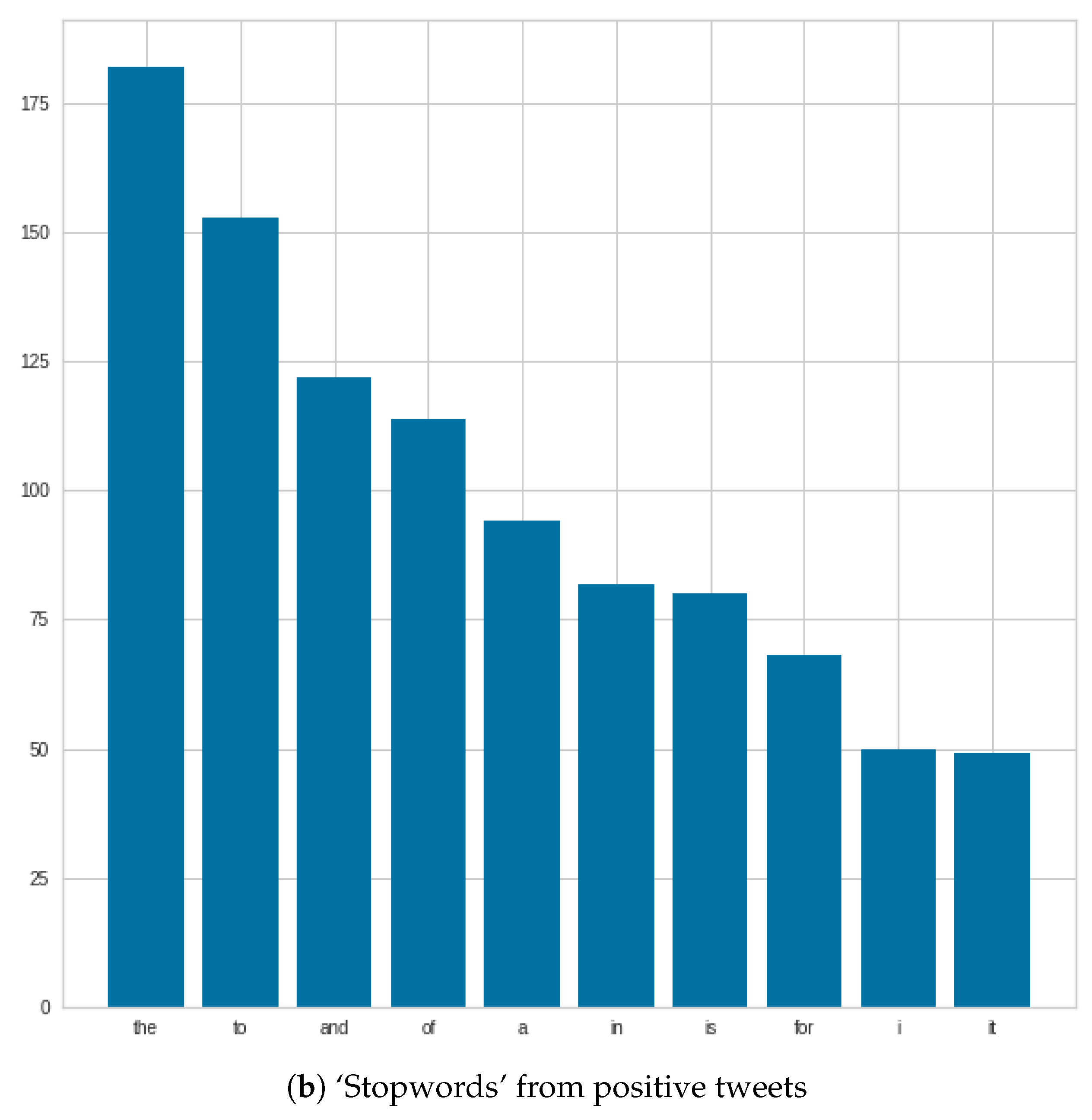
Figure 8 shows what ‘stopwords’ occurred in September for negative and positive tweets. In the case of negative tweets, the first three ‘stopwords’ are the same as in August. In the case of positive tweets, the number of ‘the’ ‘stopwords’ are increased, compared to the number of August. The third place of “a” can be mentioned, which was at fifth place in August.
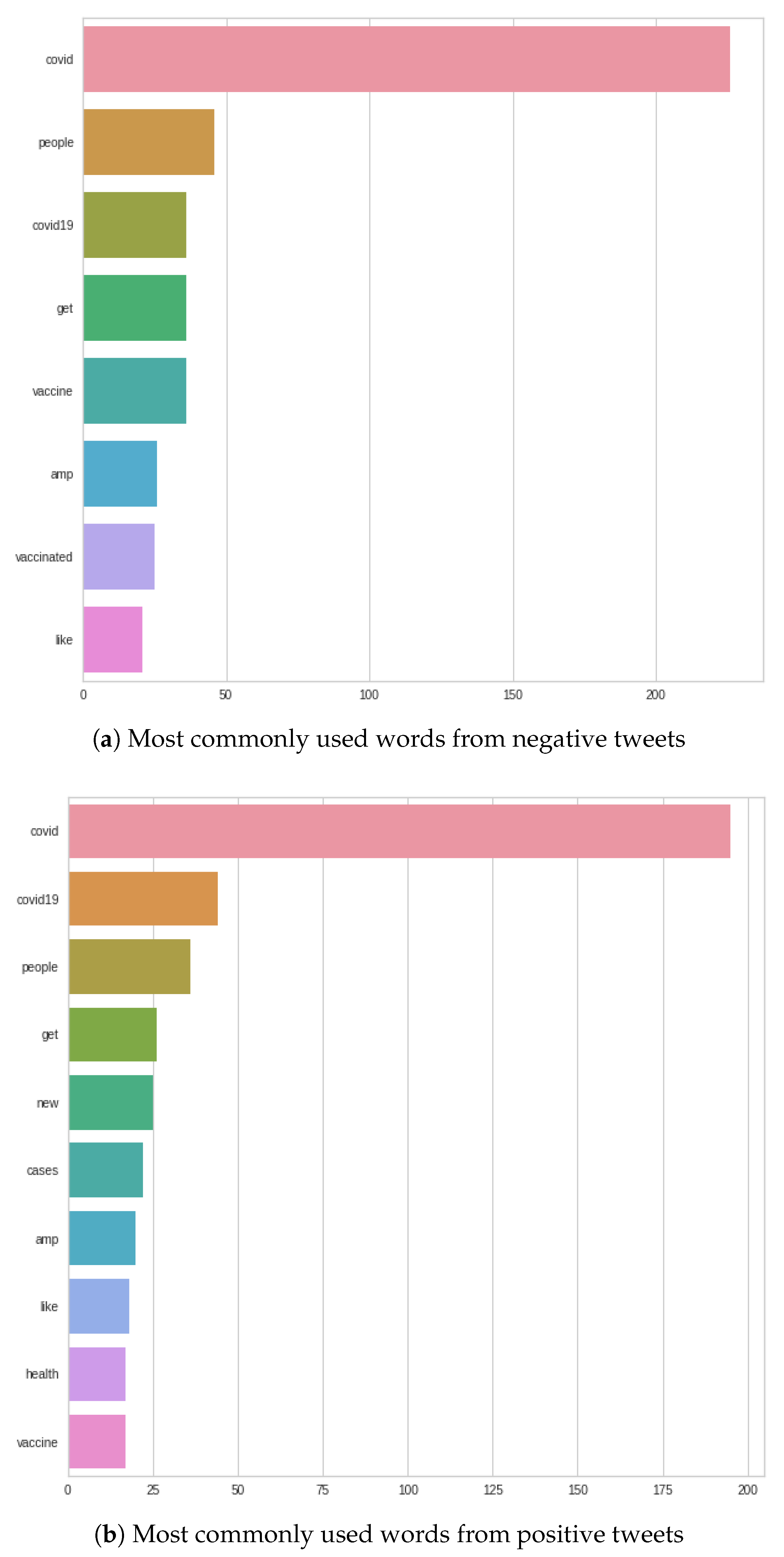
Figure 9 shows that even in September, the word ‘COVID’ completely dominated the tweets as well. In the case of negative tweets, ‘COVID’ is followed by the following three words: ‘people’, ‘COVID-19’, and ‘get’. In positive tweets, after ‘COVID’, these three words feature: ‘COVID-19’, ‘people’ and ‘get’. For both negative and positive words, the three most common words following the word ‘COVID’ are the same. There is a difference in the order—for negative tweets, the word ‘people’ is the first after ‘COVID’, and in positive words, ‘people’ is second in the queue after ‘COVID’; the first is ‘COVID-19’.
In the case of negative tweets, it should be noted that the word ‘vaccine’ was significantly ahead compared to the August results. In contrast to the positive words, the word ‘vaccine’ slid significantly backwards, and the word ‘cases’ moved forward; plus, the word of ‘health’ appeared in the plot, which was not displayed previously.
Compared to August, only small changes are seen, and the plots describe what words occur in tweets on the topic of COVID-19, and we can get an idea about the topics people are interested in, and how they describe their opinions about it.

6.3. Part of Speech Tags and Dependency Graph

After analyzing the different words, for both negative and positive tweets, it is definitely worth conducting a full part of speech analysis of which elements build up the negative and positive tweets.
As we have mentioned earlier, in some cases, a dependency graph can be used to see the actual relationships between words and to draw conclusions from them. Therefore, for the tweets with the most followers, we created a dependency graph from the datasets.

6.3.1. August

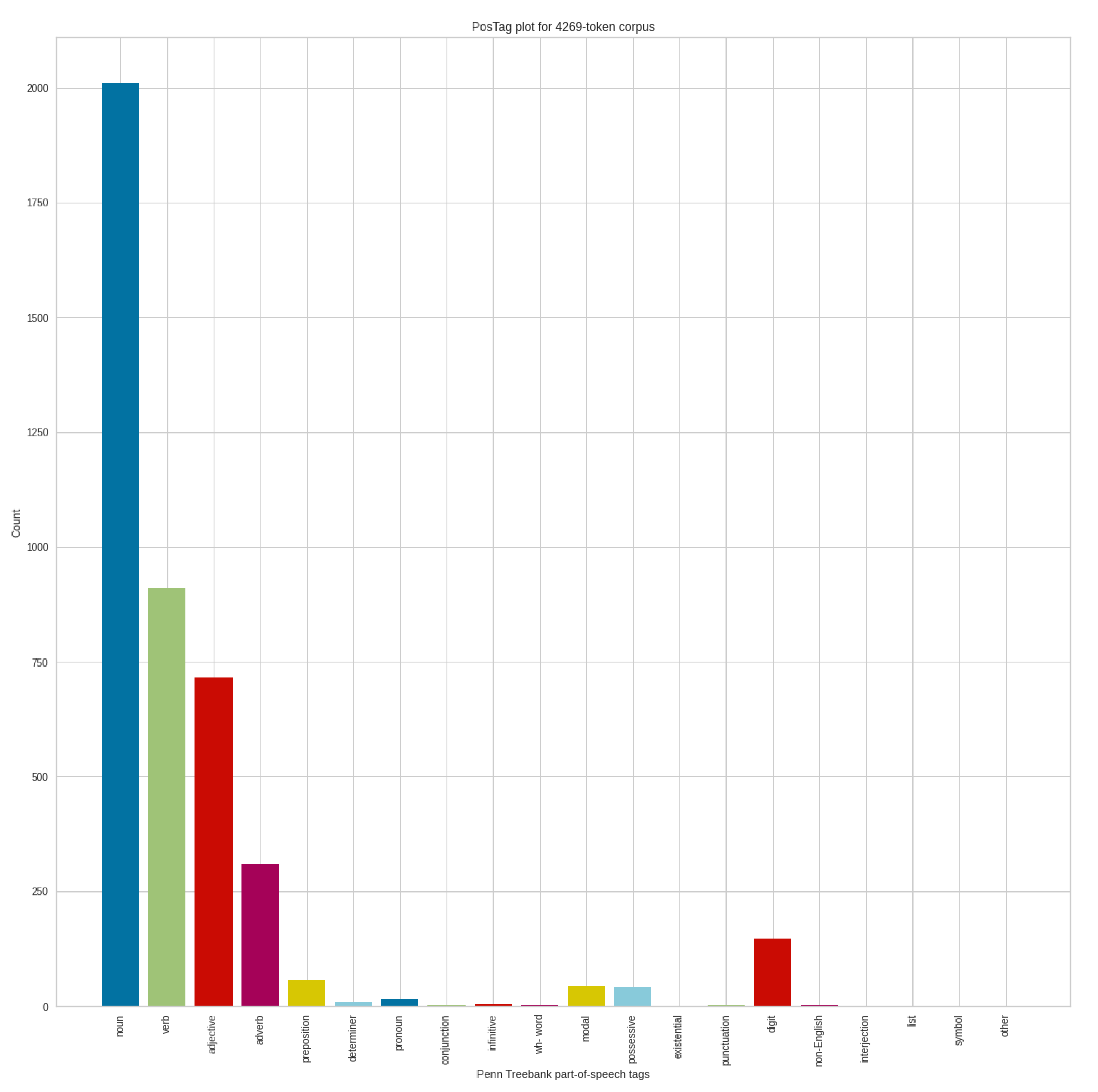
Figure 10 shows that the analysis was done with 4269 token corpus in the case of negative tweets, where the number of nouns exceeds two thousand. This is followed by verbs, adjectives and adverbs. The number of digits can also be highlighted.
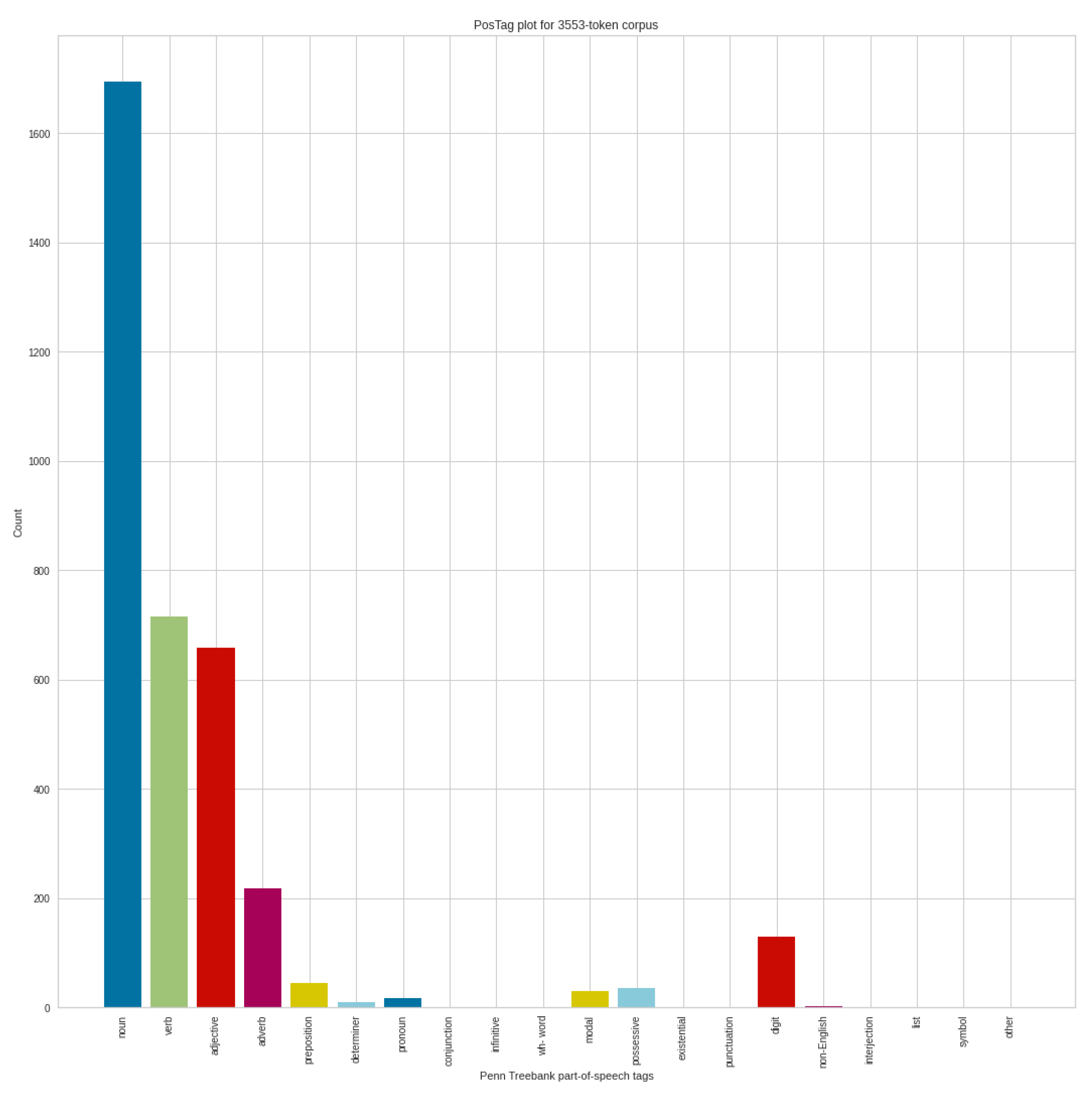
Figure 11 shows the part of speech analysis results from August on the positive tweets, which contain 3553 token corpus. Of course, the number of nouns is the most prominent here as well, followed by verbs, adjectives, and adverbs. We cannot see unusual results here either. Comparing the negative and positive POS analyses in August, we can mainly see the differences in the proportions, both in each POS group, and in the number of tokens that can be analyzed.
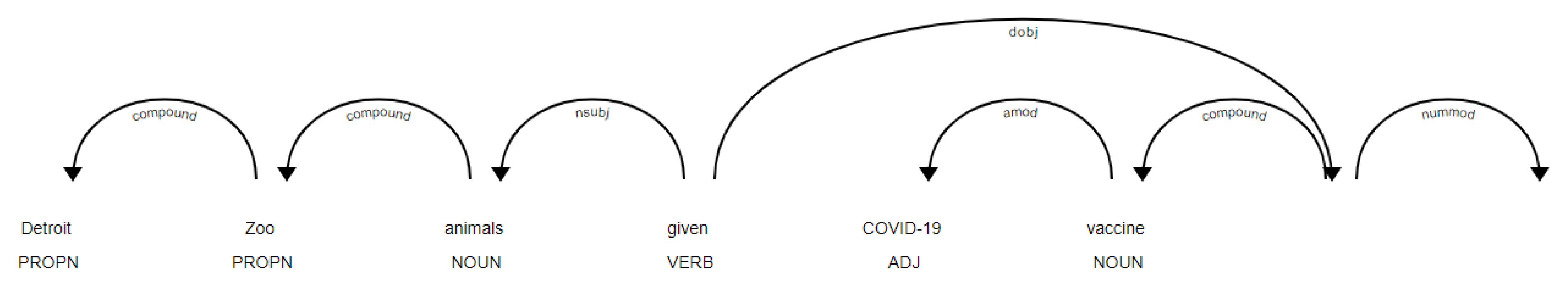
Following the POS analyses, let’s look at the results of the dependency graph (Figure 12 shows the structure of the tweet), using the positive twitter post with the most followers from the August dataset. There are two links at the end of the tweet; this is covered in the figure.

6.3.2. September

Figure 13 shows the POS analysis of the negative tweets in the September dataset, which includes 4353 token corpus. The structure of the analysis, of course, is similar to previous analyses, in the same way that the noun dominates, followed by verbs, adjectives and adverbs. If we compare the August negative POS results with the POS analysis results of the September negative tweets, we can see shifts. In addition to the increase in the number of nouns, the number of adjectives produced a more serious increase. In addition, minimal movements are noticeable in the other POS categories as well.
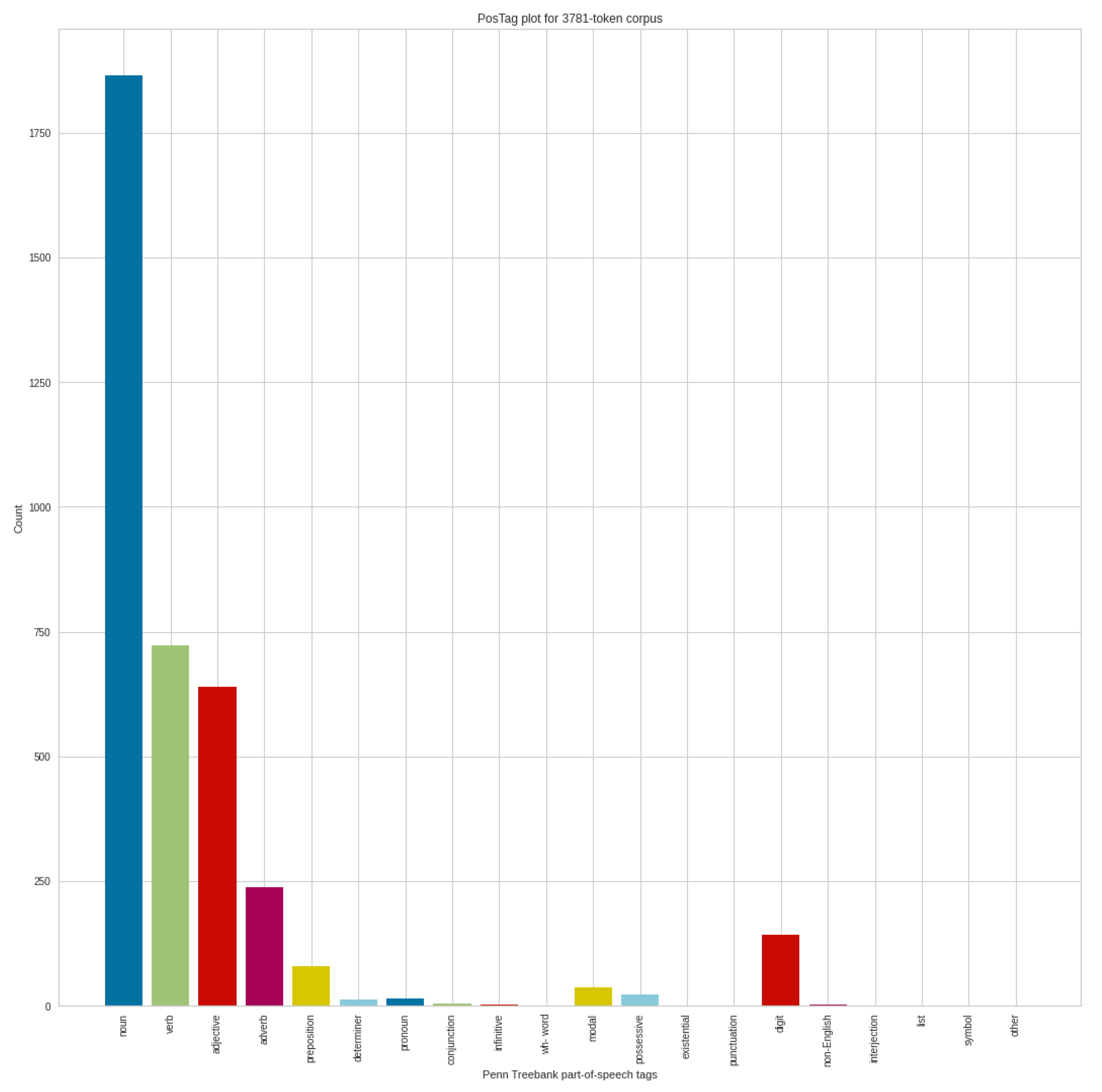
Figure 14 shows the POS analysis of the positive tweets in September, where 3781 token corpus were identified. Compared to the POS results of negative tweets, the order of the POS categories is the same. In addition to the decrease in the number of nouns, we can also see a significant decrease in the case of verbs, adjectives and adverbs. Of course, the smaller number from the tokenization process also plays a role in this, which is again a change or difference in the structure of tweets.
Comparing the positive POS results in August and the positive POS results in September, it can be seen that the number of tokens were similarly reduced compared to the results obtained in the negative cases. This already draws attention to significant differences in the words of the texts of negative and positive tweets. Comparing the POS categories for the positive tweets in August and September, we can see decreases again in verbs, and an increase in the number of nouns and adjectives.
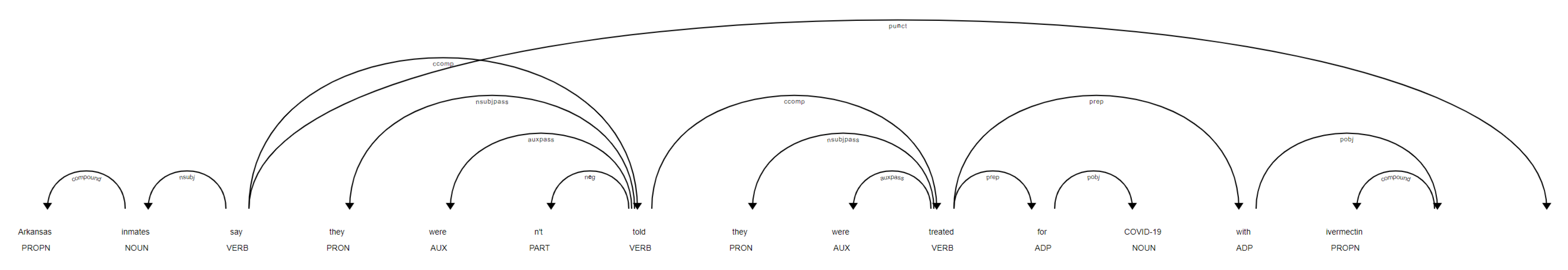
Following the POS analyses, let’s look at the results of the dependency graph. (Figure 15) In this case, a fairly long tweet has reached the most people directly, so here, we would like to illustrate that the method can be used for a large and aggregate sentence, or sentences. There are two links at the end of the tweet; this is covered in the figure.
With the help of part of speech and word analyses, which examine a deeper structure following the sentiment analysis, we already have a picture of the tweets, which were written during the given periods. What characterizes the negative and positive tweets, are what differences appear between positive and negative tweets in a given period. We could see what words occurred most often in the periods for both positive and negative tweets, and what differences appear in the tweets written on the same topic in the two periods. The POS analysis even showed the structure of the tweets, and how many differences there are between the texts of the positive and negative tweets, which occurred in the case of tokenization first, and the number of tokens in positive cases is significantly lower.
Based on the information extraction analyses and results, it may be worthwhile to include other disciplines, such as psychology or linguistics in future work, and expand the analyses purposefully.
In the next section, we explore the results with Named Entity Recognition to gain more detailed information.

6.4. Named Entity Recognition Results

We continue to use the RNN results, continuing the analyses what we started in the information extraction section. Thus, the RNN results still aggregate to the positive and negative parts.

6.4.1. August

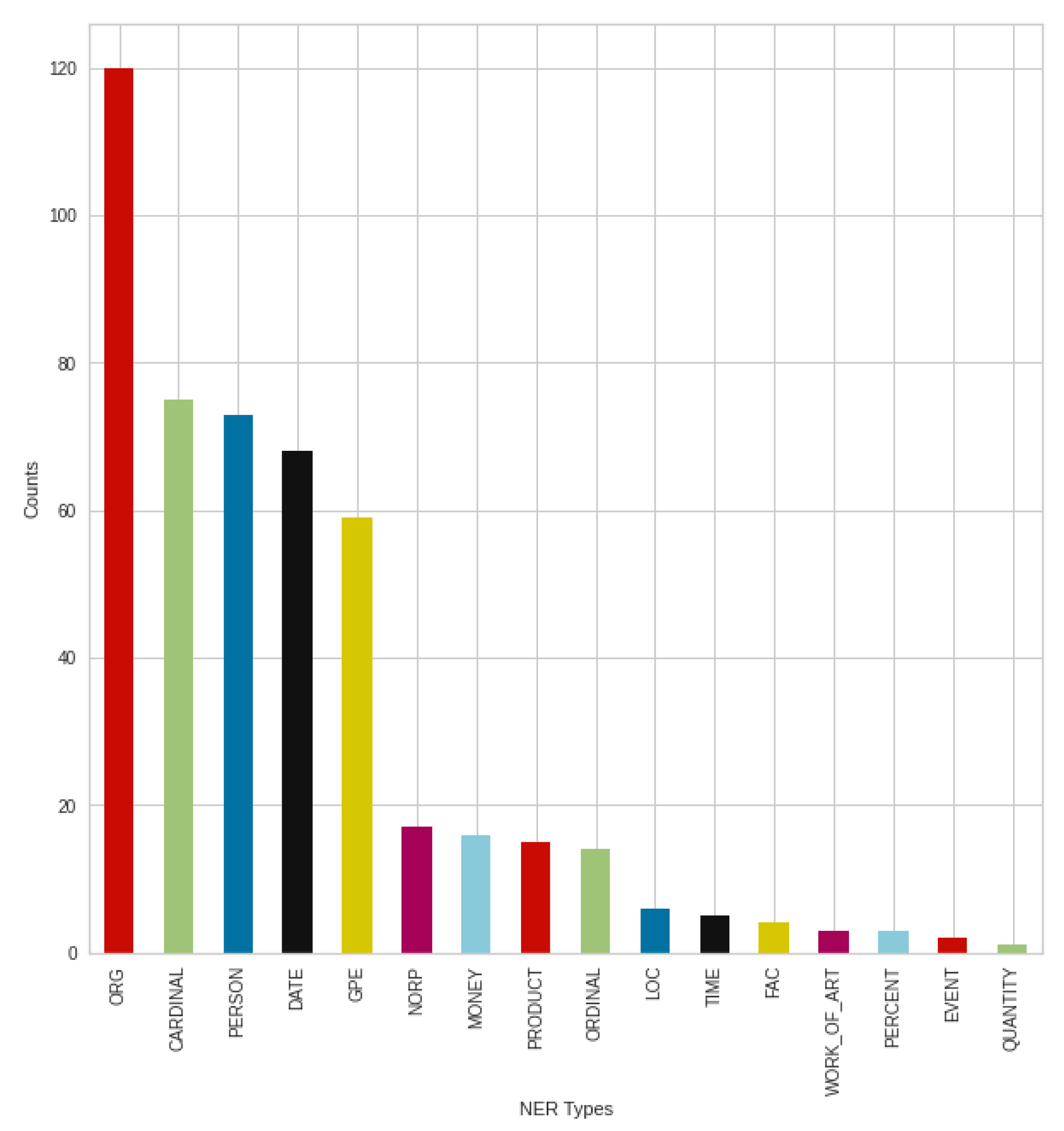
Figure 16 shows the negative tweets posted in August broken down into NER types, to see how these posts are structured, and what people mention primarily on the topic of COVID-19. In most cases, various organizations, agencies, and institutions were mentioned (‘ORG’). This is followed by countries, states, and cities (‘GPE’). In addition, numbers (’CARDINAL’—Numerals that do not fall under another type) and people/persons (‘PERSON’) followed these types before dates (‘DATE’). After different organizations, which is an outstanding result, the types that follow are very close results. Based on the results, money (‘MONEY’) and various products (‘PRODUCT’) were mentioned less at the time.
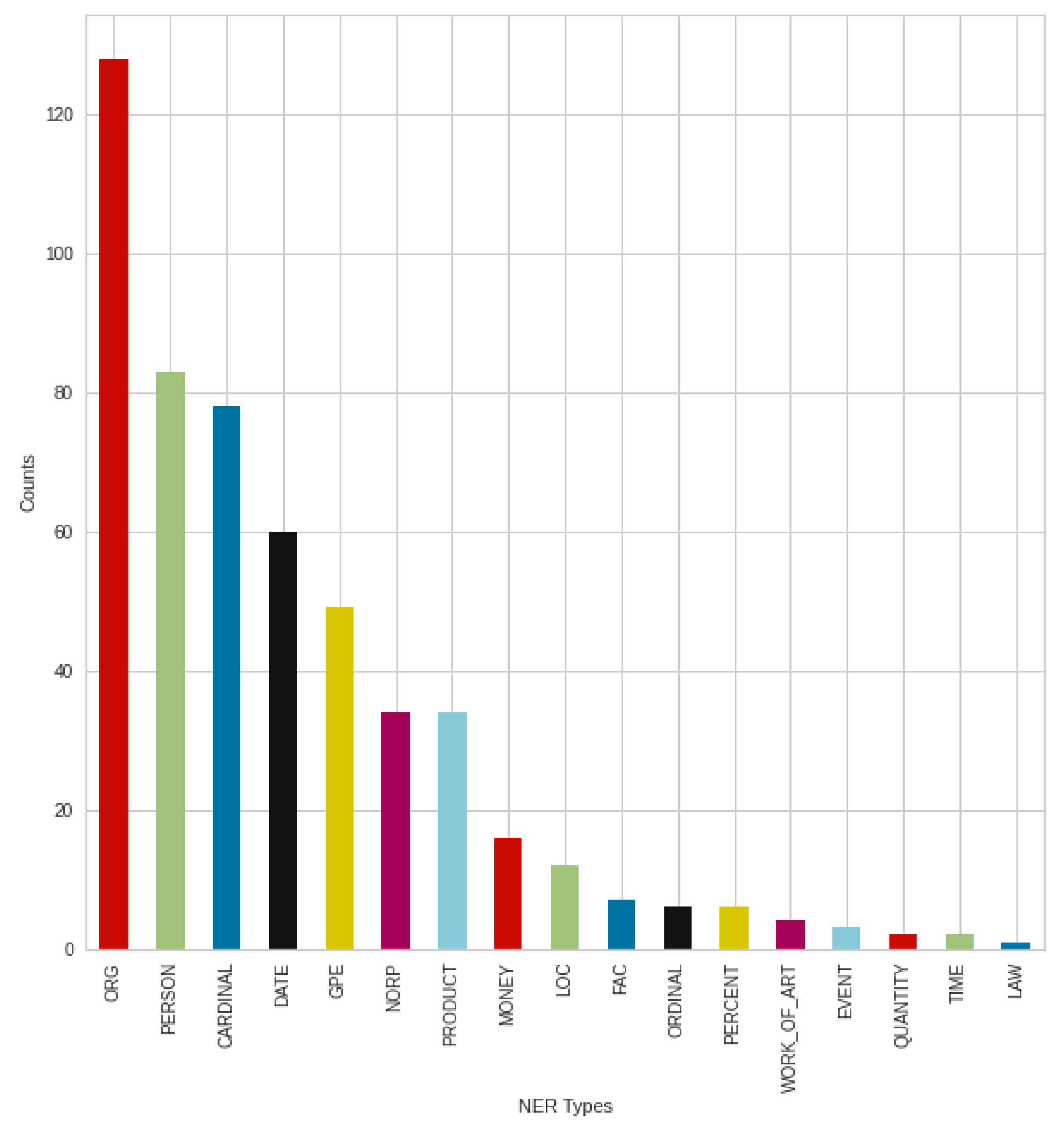
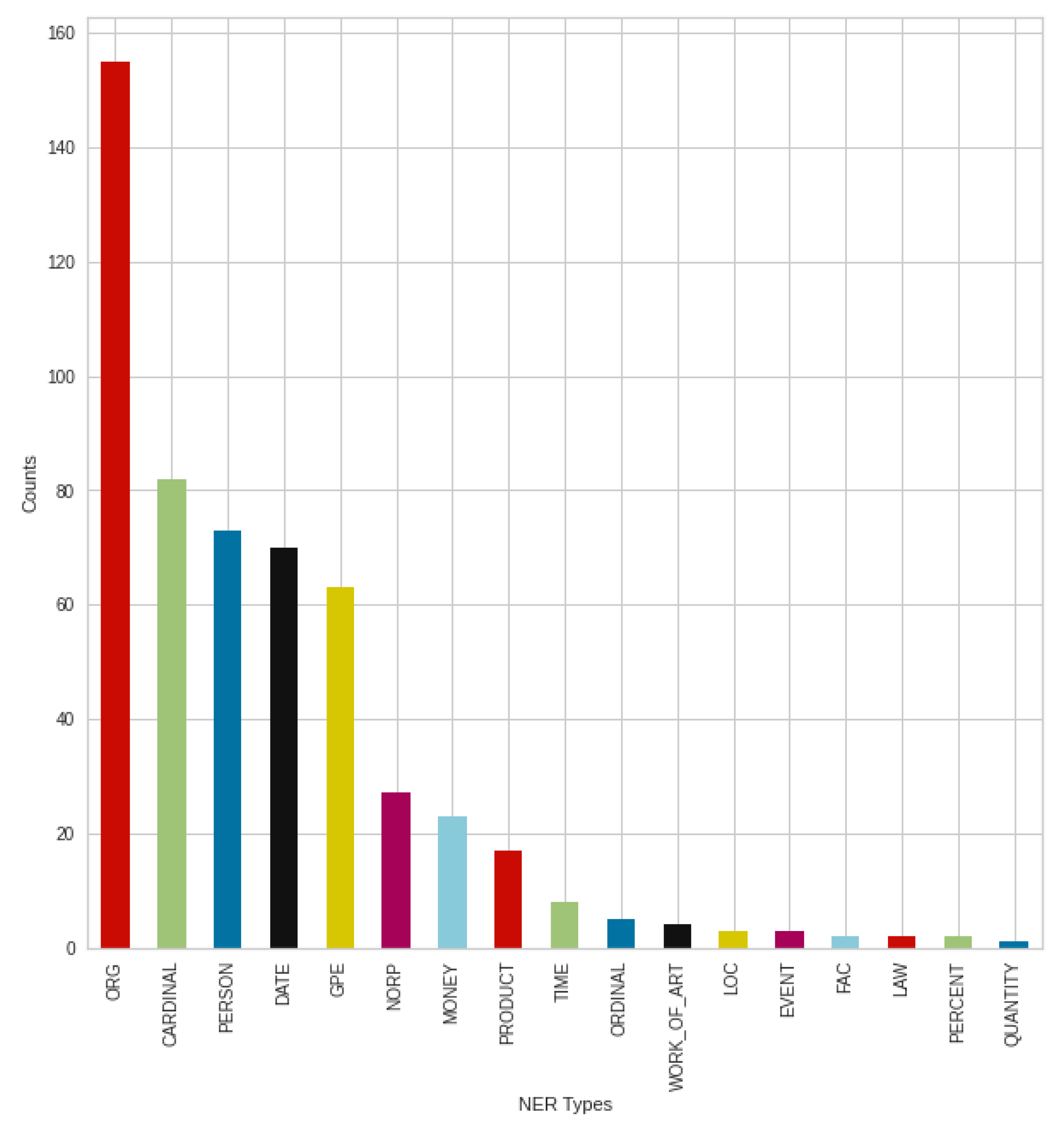
Figure 17 shows the breakdown of August positive tweets into NER types. In this case, the organizations, companies, institutions, etc. (‘ORG’) produced an outstanding result, just like in negative tweets. This is followed by a more significant rearrangement. Meanwhile, in the case of negative tweets, the type of countries, states, cities (‘GPE’) was the second strongest NER type; in positive cases, the numbers type (‘CARDINAL’) was the second strongest NER type, and the countries, states, cities were only the fifth, which is a significant difference. Furthermore, for positive tweets, the third strongest was the ‘PERSON’ type, followed by the dates (‘DATE’).
These results suggest that people are actively talking about news, events, sharing what they have read about the topic and arguing for their opinions, which they are also trying to support, to confirm their information.

6.4.2. September

Figure 18 shows the result of the negative tweets posted in September, broken down into NER types, where once again an outstanding result from organizations, companies, institutions (‘ORG’) can be seen. This is followed by the types of persons (‘PERSON’) and numbers (‘CARDINAL’). Contrary to previous August results, there was an increase in the type of nationalities or religious or political groups (‘NORP’), similar to the type of products (‘PRODUCT’). However, the trend from August can still be seen, with minimal changes in the strongest types.
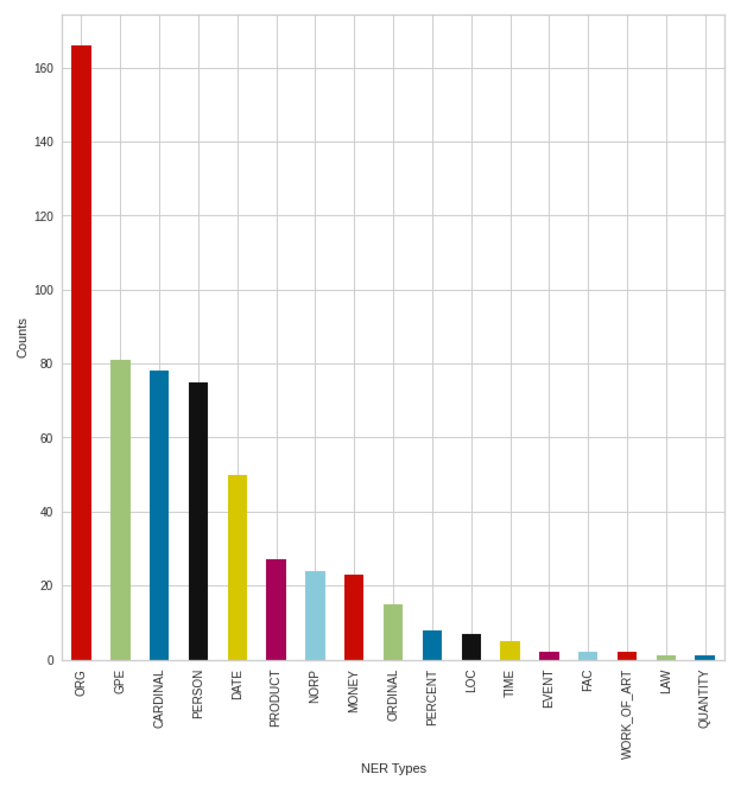
The breakdown into NER types of the positive tweets shown in Figure 19. In the case of the formation of types, this is the same as the previous August trend, especially in the case of the strongest types. If we compare the negative and positive results in September, we can see a rearrangement in the case of the less mentioned types, and a setback of the nationalities or religious or political groups (‘NORP’) type. However, this is mainly the setback of products type (‘PRODUCT’) in the positive case, which can be highlighted.

6.4.3. NER Type ‘GPE’—Deep Analysis

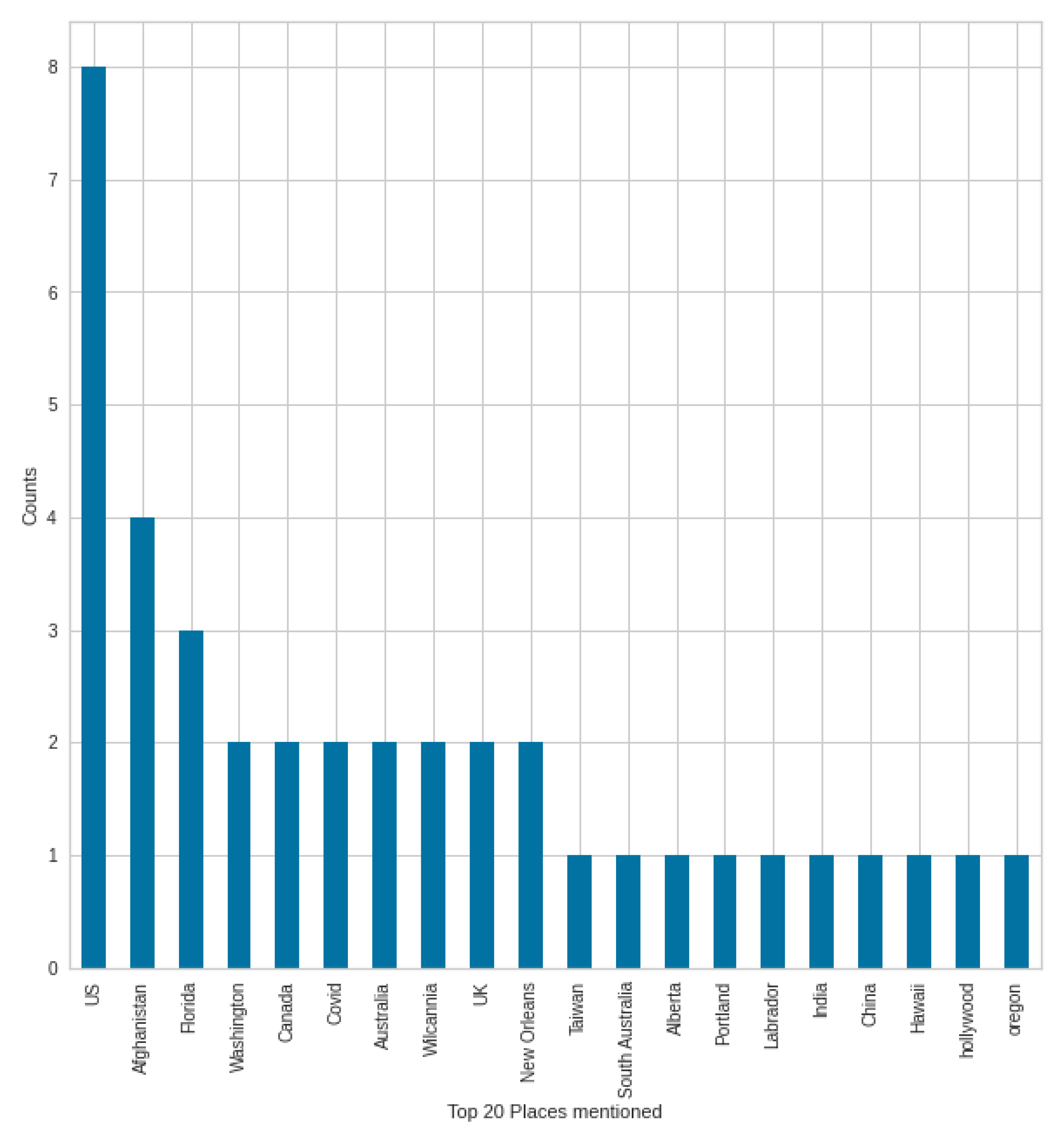
In the case of NER types, the elements of the GPE (countries, states, cities) type were mentioned the second most often in the case of negative tweets in August, which was only the fifth most often mentioned in the case of positive tweets. Therefore, we supplement the analysis with the words mentioned in the GPE type in August, in both negative and positive tweets, to see what might have resulted in this. It is possible to extend any type shown in the figure.
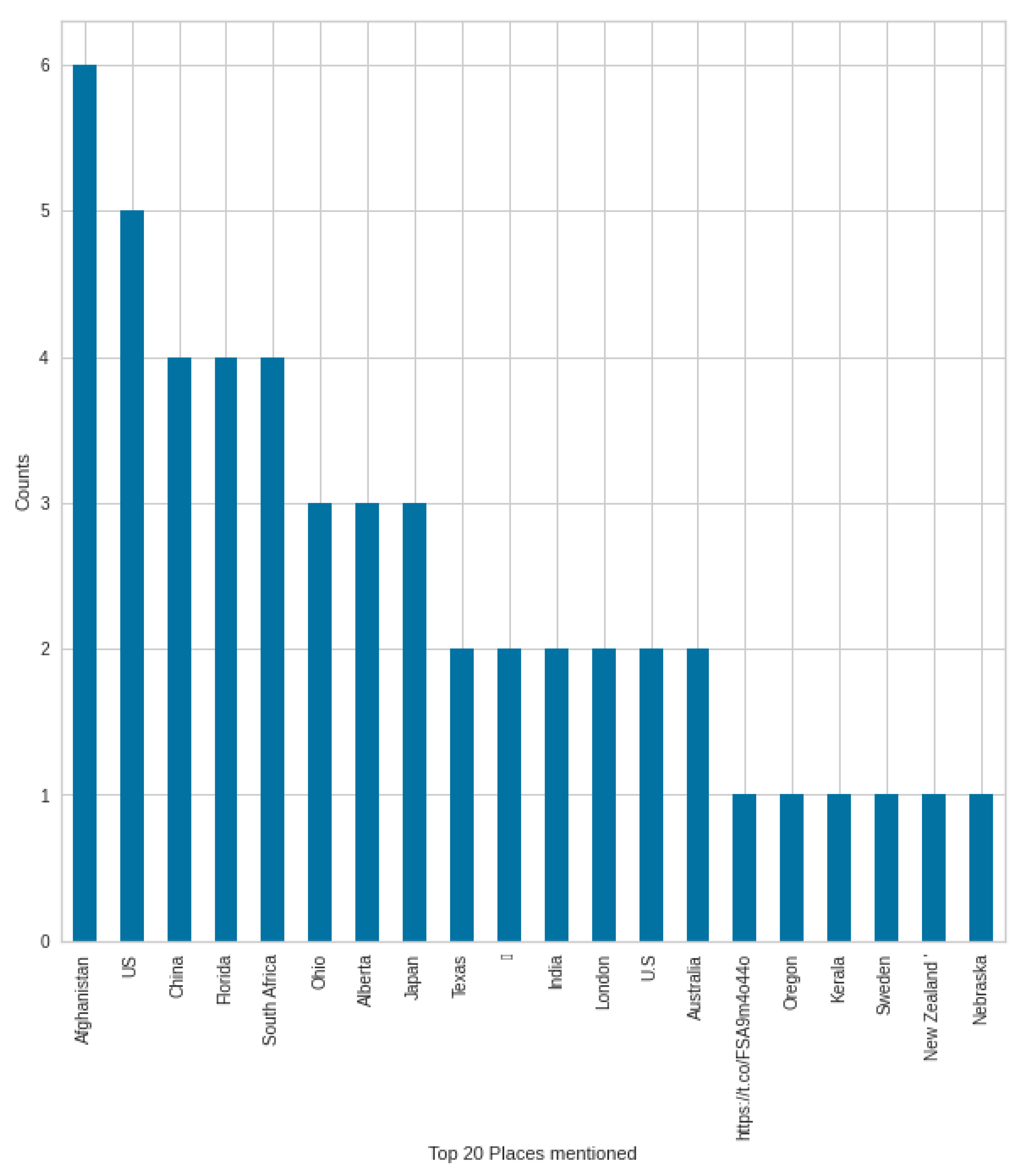
Figure 20 shows the top 20 GPE for negative tweets. In the other Figure 21, we can see the GPEs mentioned in the case of positive tweets. In a negative case, the most mentioned country was Afghanistan, which may come as a surprise at first, but at the time, all media platforms were dealing with the Afghan withdrawal and the consequences, which also had an impact on COVID-19-themed tweets. Afghanistan was followed by the United States, China, and the state of Florida. In positive tweets, Afghanistan was the second after the United States; the third was Florida state. COVID-19 is different in countries and states, and this creates a different situation. Not surprisingly, these are mentioned in the tweets, and the unique situation is given by the situation in Afghanistan in this case—which was a unique situation at the end of the summer.
With further analyses, it was possible to explore explanations, details and information in addition to the sentiment analysis, which gives a much deeper picture of the real sentiment results of the given period, and what shaped these sentiment results.

7. Discussion and Conclusions

7.1. Conclusion

In this work, we used different models for sentiment analysis to determine how people relate to the topic of COVID-19 on social media, primarily Twitter. We have created several models: BERT, RNN, NLTK—VADER and TextBlob, to analyze “fresh” datasets. The primary goal was to work with the latest data for the period under study, so we always created the datasets according to a given limit number with the ’COVID’ keyword, and the given time period of the analyses.
The sentiment analysis was extended. In addition to the usual ‘positive’, ‘neutral’, and ‘negative’ categories, we extended that with ‘strongly positive and negative’ and ’weakly positive and negative’ categories, to detect smaller sentiment movements within the positive and negative categories when comparing the sentiment results of different time intervals.
BERT provided a comparison result for our other models, where the results of the RNN model were the most approximated to the results of BERT. Thus, we performed additional information extraction and named entity recognition analyses on the sentiment categorized and labeled results by RNN, to get a deeper picture of sentiment analysis. How people write/build their tweets, what is characteristic of their writing, what is the word usage of positive and negative tweets, what places, people and more were mentioned, as well as which events may affect their tweets. Thus, we obtained a detailed analytical result on how the result of the emotional analysis developed.
The sentiment outcomes of the late August and early September period that we examined and extended by information extraction and named entity recognition analyses, explained some of the sentiment changes between the two study periods, and examined and provided a detailed picture of tweets. These analyses also give a whole new picture to traditional sentiment analysis.

7.2. Future Work

As future work, very interesting and valuable results could be achieved by involving additional disciplines such as linguistics or psychology, and expanding the research with further targeted analyses.
By introducing new classifications, analyses, and keeping the current analyses up to date, a new extended sentiment analysis library or wrapper could be created. This could extend and simplify sentiment analysis using multiple models, and it could also provide additional analyses to interpret and manage the data. This can even provide specialized analyses for different areas as well.

Author Contributions

Conceptualization, L.N., A.K.; methodology, L.N., A.K.; software, L.N.; validation, L.N., A.K.; investigation, L.N., A.K.; writing—original draft preparation, L.N., A.K.; writing—review and editing, L.N., A.K.; supervision, A.K.; project administration, A.K. All authors have read and agreed to the published version of the manuscript.

Funding

The project has been supported by the European Union, co-financed by the European Social Fund (EFOP-3.6.3-VEKOP-16-2017-00002). This research was also supported by grants of the ‘Application Domain Specific Highly Reliable IT Solutions’ project, which has been implemented with the support provided from the National Research, Development and Innovation Fund of Hungary, financed under the Thematic Excellence Programme TKP2020-NKA-06 (National Challenges Subprogramme) funding scheme.

Institutional Review Board Statement

Not applicable.

Informed Consent Statement

Not applicable.

Data Availability Statement

The analysis was performed on newly created datasets. The code for this scraping script, as well as the analysis notebook, a previously taught usable RNN model, and the datasets, which needed to teach BERT, can be found here: https://github.com/NemesLaszlo/Social-Media-Analysis-based-on-COVID-19-with-Sentiment-Analysis-NER-and-Information-Extraction, accessed on 1 October 2021.

Conflicts of Interest

The authors declare no conflict of interest.

Abbreviations

The following abbreviations are used in this manuscript:
NLPNatural Language Processing
NLTKNatural Language Toolkit
VADERValence Aware Dictionary and Sentiment Reasoner
BERTBidirectional Encoder Representations from Transformers
RNNRecurrent Neural Network
LSTMLong Short-Term Memory
IEInformation Extraction
NERNamed Entity Recognition
POSPart of Speech

References

  1. Ptaszynski, M.; Masui, F.; Fukushima, Y.; Oikawa, Y.; Hayakawa, H.; Miyamori, Y.; Takahashi, K.; Kawajiri, S. Deep Learning for Information Triage on Twitter. Appl. Sci. 2021, 11, 6340. [Google Scholar] [CrossRef]
  2. Iglesias, C.A.; Moreno, A. Sentiment Analysis for Social Media. Appl. Sci. 2019, 9, 5037. [Google Scholar] [CrossRef] [Green Version]
  3. Jianqiang, Z.; Xiaolin, G.; Xuejun, Z. Deep Convolution Neural Networks for Twitter Sentiment Analysis. IEEE Access 2018, 6, 23253–23260. [Google Scholar] [CrossRef]
  4. Jnoub, N.; Al Machot, F.; Klas, W. A Domain-Independent Classification Model for Sentiment Analysis Using Neural Models. Appl. Sci. 2020, 10, 6221. [Google Scholar] [CrossRef]
  5. Wang, J.-H.; Liu, T.-W.; Luo, X. Combining Post Sentiments and User Participation for Extracting Public Stances from Twitter. Appl. Sci. 2020, 10, 8035. [Google Scholar] [CrossRef]
  6. Chandra Pandey, A.; Singh Rajpoot, D.; Saraswat, M. Twitter Sentiment Analysis Using Hybrid Cuckoo Search Method. Inf. Process. Manag. 2017, 53, 764–779. [Google Scholar] [CrossRef]
  7. Yasir, M.; Durrani, M.Y.; Afzal, S.; Maqsood, M.; Aadil, F.; Mehmood, I.; Rho, S. An Intelligent Event-Sentiment-Based Daily Foreign Exchange Rate Forecasting System. Appl. Sci. 2019, 9, 2980. [Google Scholar] [CrossRef] [Green Version]
  8. Štrimaitis, R.; Stefanovič, P.; Ramanauskaitė, S.; Slotkienė, A. Financial Context News Sentiment Analysis for the Lithuanian Language. Appl. Sci. 2021, 11, 4443. [Google Scholar] [CrossRef]
  9. Xu, J.; Huang, F.; Zhang, X.; Wang, S.; Li, C.; Li, Z.; He, Y. Sentiment Analysis of Social Images via Hierarchical Deep Fusion of Content and Links. Appl. Soft Comput. 2019, 80, 387–399. [Google Scholar] [CrossRef]
  10. Khalid, M.; Ashraf, I.; Mehmood, A.; Ullah, S.; Ahmad, M.; Choi, G.S. GBSVM: Sentiment Classification from Unstructured Reviews Using Ensemble Classifier. Appl. Sci. 2020, 10, 2788. [Google Scholar] [CrossRef] [Green Version]
  11. Rizkallah, S.; Atiya, A.F.; Shaheen, S. A Polarity Capturing Sphere for Word to Vector Representation. Appl. Sci. 2020, 10, 4386. [Google Scholar] [CrossRef]
  12. Han, K.-X.; Chien, W.; Chiu, C.-C.; Cheng, Y.-T. Application of Support Vector Machine (SVM) in the Sentiment Analysis of Twitter DataSet. Appl. Sci. 2020, 10, 1125. [Google Scholar] [CrossRef] [Green Version]
  13. Chakriswaran, P.; Vincent, D.R.; Srinivasan, K.; Sharma, V.; Chang, C.-Y.; Reina, D.G. Emotion AI-Driven Sentiment Analysis: A Survey, Future Research Directions, and Open Issues. Appl. Sci. 2019, 9, 5462. [Google Scholar] [CrossRef] [Green Version]
  14. Park, S.; Woo, J. Gender Classification Using Sentiment Analysis and Deep Learning in a Health Web Forum. Appl. Sci. 2019, 9, 1249. [Google Scholar] [CrossRef] [Green Version]
  15. Khai Tran, T.; Thi Phan, T. Deep Learning Application to Ensemble Learning—The Simple, but Effective, Approach to Sentiment Classifying. Appl. Sci. 2019, 9, 2760. [Google Scholar] [CrossRef] [Green Version]
  16. Li, W.; Li, D.; Yin, H.; Zhang, L.; Zhu, Z.; Liu, P. Lexicon-Enhanced Attention Network Based on Text Representation for Sentiment Classification. Appl. Sci. 2019, 9, 3717. [Google Scholar] [CrossRef] [Green Version]
  17. Devlin, J.; Chang, M.-W.; Lee, K.; Toutanova, K. BERT: Pre-Training of Deep Bidirectional Transformers for Language Understanding. arXiv 2019, arXiv:1810.04805. [Google Scholar]
  18. Han, X.; Wang, J.; Zhang, M.; Wang, X. Using Social Media to Mine and Analyze Public Opinion Related to COVID-19 in China. Int. J. Environ. Res. Public Health 2020, 17, 2788. [Google Scholar] [CrossRef] [Green Version]
  19. Alamoodi, A.H.; Zaidan, B.B.; Zaidan, A.A.; Albahri, O.S.; Mohammed, K.I.; Malik, R.Q.; Almahdi, E.M.; Chyad, M.A.; Tareq, Z.; Albahri, A.S.; et al. Sentiment Analysis and Its Applications in Fighting COVID-19 and Infectious Diseases: A Systematic Review. Expert Syst. Appl. 2021, 167, 114155. [Google Scholar] [CrossRef]
  20. Sattar, N.S.; Arifuzzaman, S. COVID-19 Vaccination Awareness and Aftermath: Public Sentiment Analysis on Twitter Data and Vaccinated Population Prediction in the USA. Appl. Sci. 2021, 11, 6128. [Google Scholar] [CrossRef]
  21. Amanatidis, D.; Mylona, I.; Kamenidou, I.; Mamalis, S.; Stavrianea, A. Mining Textual and Imagery Instagram Data during the COVID-19 Pandemic. Appl. Sci. 2021, 11, 4281. [Google Scholar] [CrossRef]
  22. Gutiérrez-Esparza, G.O.; Vallejo-Allende, M.; Hernández-Torruco, J. Classification of Cyber-Aggression Cases Applying Machine Learning. Appl. Sci. 2019, 9, 1828. [Google Scholar] [CrossRef] [Green Version]
  23. Rodríguez-González, A.; Tuñas, J.M.; Prieto Santamaría, L.; Fernández Peces-Barba, D.; Menasalvas Ruiz, E.; Jaramillo, A.; Cotarelo, M.; Conejo Fernández, A.J.; Arce, A.; Gil, A. Identifying Polarity in Tweets from an Imbalanced Dataset about Diseases and Vaccines Using a Meta-Model Based on Machine Learning Techniques. Appl. Sci. 2020, 10, 9019. [Google Scholar] [CrossRef]
  24. Wang, T.; Lu, K.; Chow, K.P.; Zhu, Q. COVID-19 Sensing: Negative Sentiment Analysis on Social Media in China via BERT Model. IEEE Access 2020, 8, 138162–138169. [Google Scholar] [CrossRef]
  25. Catelli, R.; Gargiulo, F.; Casola, V.; De Pietro, G.; Fujita, H.; Esposito, M. Crosslingual Named Entity Recognition for Clinical De-Identification Applied to a COVID-19 Italian Data Set. Appl. Soft Comput. 2020, 97, 106779. [Google Scholar] [CrossRef] [PubMed]
  26. López-Úbeda, P.; Díaz-Galiano, M.C.; Martín-Noguerol, T.; Luna, A.; Ureña-López, L.A.; Martín-Valdivia, M.T. COVID-19 Detection in Radiological Text Reports Integrating Entity Recognition. Comput. Biol. Med. 2020, 127, 104066. [Google Scholar] [CrossRef] [PubMed]
  27. Wang, X.; Song, X.; Li, B.; Guan, Y.; Han, J. Comprehensive Named Entity Recognition on CORD-19 with Distant or Weak Supervision. arXiv 2020, arXiv:2003.12218. [Google Scholar]
  28. Lybarger, K.; Ostendorf, M.; Thompson, M.; Yetisgen, M. Extracting COVID-19 Diagnoses and Symptoms from Clinical Text: A New Annotated Corpus and Neural Event Extraction Framework. Biomed. Inform. 2021, 117, 103761. [Google Scholar] [CrossRef]
  29. Jonnalagadda, S.R.; Adupa, A.K.; Garg, R.P.; Corona-Cox, J.; Shah, S.J. Text Mining of the Electronic Health Record: An Information Extraction Approach for Automated Identification and Subphenotyping of HFpEF Patients for Clinical Trials. Cardiovasc. Transl. Res. 2017, 10, 313–321. [Google Scholar] [CrossRef]
  30. Apostolopoulos, I.D.; Mpesiana, T.A. Covid-19: Automatic detection from X-ray images utilizing transfer learning with convolutional neural networks. Phys. Eng. Sci. Med. 2020, 43, 635–640. [Google Scholar] [CrossRef] [PubMed] [Green Version]
Figure 1. Analysis process.
Applsci 11 11017 g001
Figure 2. Analysis of sample of 500 tweets by TextBlob, using “COVID” keyword. The time periods stands between 29 August 2021 and 31 August 2021, and 2 September 2021 and 4 September 2021.
Applsci 11 11017 g002
Figure 3. Analysis of sample of 500 tweets by NLTK—VADER, using the keyword ‘COVID’. The time periods stands between 29 August 2021 and 31 August 2021, and 2 September 2021 and 4 September 2021.
Applsci 11 11017 g003
Figure 4. Analysis of sample of 500 tweets by RNN, using “COVID” keyword. The time periods stands between 29 August 2021 and 31 August 2021, and 2 September 2021 and 4 September 2021.
Applsci 11 11017 g004
Figure 5. Analysis of sample of 500 tweets by BERT, using ‘COVID’ keyword. The time periods stands between 29 August 2021 and 31 August 2021, and 2 September 2021 and 4 September 2021.
Applsci 11 11017 g005
Figure 6. Negative and positive ‘Stopwords’. The time periods stands between 29 August 2021 and 31 August 2021.
Applsci 11 11017 g006aApplsci 11 11017 g006b
Figure 7. Most commonly used words in negative and positive tweets. The time periods stands between 29 August 2021 and 31 August 2021.
Applsci 11 11017 g007aApplsci 11 11017 g007b
Figure 8. Negative and positive ‘Stopwords’. The time period stands between 2 September 2021 and 4 September 2021.
Applsci 11 11017 g008
Figure 9. Most commonly used words in negative and positive tweets. The time period stands between 2 September 2021 and 4 September 2021.
Applsci 11 11017 g009
Figure 10. Part of speech tagging for negative tweets. The time period stands between 29 August 2021 and 31 August 2021.
Applsci 11 11017 g010
Figure 11. Part of speech tagging for positive tweets. The time period stands between 29 August 2021 and 31 August 2021.
Applsci 11 11017 g011
Figure 12. Most followed user’s tweet (positive).The time period stands between 29 August 2021 and 31 August 2021.
Applsci 11 11017 g012
Figure 13. Part of speech tagging for negative tweets. The time periods stands between 2 September 2021 and 4 September 2021.
Applsci 11 11017 g013
Figure 14. Part of speech tagging for positive tweets. The time period stands between 2 September 2021 and 4 September 2021.
Applsci 11 11017 g014
Figure 15. Most followed user’s tweet (positive). The time period stands between 2 September 2021 and 4 September 2021.
Applsci 11 11017 g015
Figure 16. NER types of the negative tweets. The time period stands between 29 August 2021 and 31 August 2021.
Applsci 11 11017 g016
Figure 17. NER types of the positive tweets. The time period stands between 29 August 2021 and 31 August 2021.
Applsci 11 11017 g017
Figure 18. NER types of the negative tweets. The time period stands between 2 September 2021 and 4 September 2021.
Applsci 11 11017 g018
Figure 19. NER types of the positive tweets. The time period stands between 2 September 2021 and 4 September 2021.
Applsci 11 11017 g019
Figure 20. GPEs mentioned in negative tweets. The time period stands between 29 August 2021 and 31 August 2021.
Applsci 11 11017 g020
Figure 21. GPEs mentioned in positive tweets. The time period stands between 29 August 2021 and 31 August 2021.
Applsci 11 11017 g021
Publisher’s Note: MDPI stays neutral with regard to jurisdictional claims in published maps and institutional affiliations.

