Analytical Modeling of the Maximum Power Point with Series Resistance

Abstract

This paper presents new analytical expressions for the maximum power point voltage, current, and power that have an explicit dependence on the series resistance. An explicit expression that relates the series resistance to well-known solar cell parameters was also derived. The range of the validity of the model, as well as the mathematical assumptions taken to derive it are explained and discussed. To test the accuracy of the derived model, a numerical single-diode model with solar cell parameters whose values can be found in the latest installment of the solar cell efficiency tables was used. The accuracy of the derived model was found to increase with increasing bandgap and to decrease with increasing series resistance. An experimental validation of the analytical model is provided and its practical limitations addressed. The new expressions predicted the maximum power obtainable by the studied cells with estimated errors below $0.1\%$ compared to the numerical model, for typical values of the series resistance.

1. Introduction

Shockley’s diode equation describes how a solar cell responds to bias and illumination [1]. Analytical expressions for photovoltaic parameters, such as the open-circuit voltage, $V_{\mathrm{oc}}$, or the short-circuit current, $i_{\mathrm{sc}}$, can easily be derived from it. When series resistance is accounted for, however, the diode equation becomes an implicit expression of the current, which is not as straightforward to work with. Some work has been performed aiming to quantify analytically the effect of series resistance on various solar cell parameters. Banwell et al. showed that Lambert’s W function allows for a closed-form expression of the current when the effect of series resistance is considered [2]. Jain et al. derived, in [3], an analogue to Banwell’s expression that also accounted for the effect of shunt resistance. The latter authors later made use of this expression to derive analytical expressions for $V_{\mathrm{oc}}$ and $i_{\mathrm{sc}}$. The maximum power point (MPP) has been little explored from an analytical perspective, although some exceptions exist [4,5,6,7,8]. The reason for this lies in the fact that, when series resistance is considered, deriving an expression for the maximum power point voltage, $V_{\mathrm{mpp}}$, involves solving a transcendental equation. Such equations often do not have closed-form solutions and need to be solved numerically. It is worth mentioning the work presented in [4], where Singal was able to obtain an approximate closed-form expression of $V_{\mathrm{mpp}}$, in terms of $V_{\mathrm{oc}}$. In contrast with a numerical model, an analytical model would allow identifying the physical parameters affecting the MPP. Accounting for the series resistance in the analytical model for the MPP would also allow for better characterization of real solar cells. In this sense, such a model would describe the MPP with higher accuracy than other analytical models that do not account for the effect of series resistance. The lack of an accurate analytical model for the MPP, which includes series resistance, in the scientific literature represents a research gap that this work aims to fill. To this end, a closed-form expression for the maximum power point voltage that accounts for the effect of the series resistance is derived. The starting point of the derivation is the analytical expression for the current, derived by Banwell in [2], in terms of Lambert’s W function. It is then argued that, at the maximum power point, the argument of the W function is small enough to accurately approximate the function value. This makes the transcendental problem analytically solvable. The accuracy of the derived model was found to increase with increasing bandgap energy and to decrease with increasing series resistance. From the new expression for $V_{\mathrm{mpp}}$, an analytical expression for the series resistance was then derived. Additionally, approximate analytical expressions for the maximum power point current, $i_{\mathrm{mpp}}$, and power, $P_{\mathrm{mpp}}$, were derived. Numerical results were calculated using parameters typical for seven different solar cell technologies. The accuracy of the model was tested through a comparison with reference values that were obtained from a numerical single-diode model. The results showed that the analytic model can predict the maximum power with relative errors below $0.1\%$ when compared to the numerical model, when typical values of the series resistance are used. Still, it must be kept in mind that the analytical approach derived in the present work corresponds to a one-diode model. This implies that it should not be used with solar cells that follow, e.g., the double-diode equation. For such cells, different techniques, such as those proposed in [9], should be employed. Finally, the practical limitations of the model are discussed based on its experimental validation, provided in [10]. Whereas the present work focuses on the derivation, range of validity, and theoretical limitations of the model from a formal perspective, in [10] the focus was on its experimental applicability.

To summarize, this work presents a novel approach based on the use of Lambert’s W function to obtain closed-form analytical expressions for the MPP that account for the effect of the series resistance.

2. Background

Assuming nondegenerate conditions, the total current density, i, produced by a solar cell is given by Shockley’s diode equation [11],

$$i=i_{\mathrm{G}}-i_{0}exp\left[\frac{V}{V_{\mathrm{t}}}\right],$$

(1)

where V is the voltage and $i_{\mathrm{G}}$ and $i_0$ are the generation and thermal recombination [12] currents, respectively. Here, the thermal voltage, $V_{\mathrm{t}}$, given by $q{V}_{\mathrm{t}}=kT$ with T, k, and q being the cell temperature, Boltzmann’s constant, and the electron charge, respectively, is introduced. The total power density, P, is given by the product $P=Vi$ [13]. At the maximum power point, it holds that:

$$\frac{\mathrm{d}}{\mathrm{d}V}P=i+V\frac{\mathrm{d}}{\mathrm{d}V}i=0.$$

(2)

Khanna et al. found that Equation (2) is solved by [14,15]:

$$V_{\mathrm{mpp}}=V_{\mathrm{t}}\left(\mathrm{W}\left[\frac{i_{\mathrm{G}}}{i_0}e\right]-1\right),$$

(3)

where $\mathrm{W}\left(x\right)$, defined by $x=\mathrm{W}\left(x{e}^x\right)$, is Lambert’s W function [16]. An expression for the maximum power point current, $i_{\mathrm{mpp}}$, can be obtained by inserting Equation (3) into Equation (1), and an expression for the maximum power, $P_{\mathrm{mpp}}$, is obtained from the product $P_{\mathrm{mpp}}=V_{\mathrm{mpp}}{i}_{\mathrm{mpp}}$. This yields [14,15]:

$$i_{\mathrm{mpp}}=i_{\mathrm{G}}\left(1-\frac{1}{\mathrm{W}\left[\frac{i_{\mathrm{G}}}{i_0}e\right]}\right),$$

(4)

$$P_{\mathrm{mpp}}=i_{\mathrm{G}}{V}_{\mathrm{t}}\left(\mathrm{W}\left[\frac{i_{\mathrm{G}}}{i_0}e\right]-2+\frac{1}{\mathrm{W}\left[\frac{i_{\mathrm{G}}}{i_0}e\right]}\right).$$

(5)

When series resistance is accounted for, Equation (1) becomes [13]:

$$i=i_{\mathrm{G}}-i_{0}exp\left[\frac{V+ir}{V_{\mathrm{t}}}\right],$$

(6)

where r is the cell series resistance $(\left[r\right]=\Omega ·{\mathrm{cm}}^2)$. Banwell et al. proved in [2] that Lambert’s W function allows for an explicit expression for i. Defining the voltages $V_{\mathrm{G}}$ and $V_0$ as $V_{\mathrm{G}}=i_{\mathrm{G}}r$ and $V_0=i_{0}r$, Equation (6) becomes [2]:

$$i=i_{\mathrm{G}}-\frac{V_{\mathrm{t}}}{r}\mathrm{W}\left[\frac{V_0}{V_{\mathrm{t}}}exp\left[\frac{V_{\mathrm{G}}}{V_{\mathrm{t}}}+\frac{V}{V_{\mathrm{t}}}\right]\right],$$

(7)

from which it can be seen that in the limit $r\to 0$, Equation (1) is recovered.

3. The Maximum Power Point

Let $z\left(V\right)$ denote the argument of Lambert’s W function in Equation (7), and let $z_{\mathrm{mpp}}:=z\left(V_{\mathrm{mpp}}\right)$. Inserting Equation (7) into Equation (2) yields:

$$\begin{array}{cc}\hfill 0={\left[i+V\frac{\mathrm{d}}{\mathrm{d}V}i\right]}_{V=V_{\mathrm{mpp}}}& =i\left(V_{\mathrm{mpp}}\right)+V_{\mathrm{mpp}}\frac{-V_{\mathrm{t}}}{r}\frac{\mathrm{W}\left(z_{\mathrm{mpp}}\right)}{1+\mathrm{W}\left(z_{\mathrm{mpp}}\right)}{\left[\frac{\mathrm{d}}{\mathrm{d}V}logz\right]}_{V=V_{\mathrm{mpp}}}\hfill \\ \hfill \\ \hfill & =i_{\mathrm{G}}-\frac{V_{\mathrm{t}}}{r}\mathrm{W}\left(z_{\mathrm{mpp}}\right)-\frac{V_{\mathrm{mpp}}}{r}\frac{\mathrm{W}\left(z_{\mathrm{mpp}}\right)}{1+\mathrm{W}\left(z_{\mathrm{mpp}}\right)}\hfill \\ \hfill \\ \hfill & =\frac{V_{\mathrm{t}}}{r}\mathrm{W}\left(z_{\mathrm{mpp}}\right)\left[\frac{1}{\mathrm{W}\left(z_{\mathrm{mpp}}\right)}\frac{i_{\mathrm{G}}r}{V_{\mathrm{t}}}-1-\frac{V_{\mathrm{mpp}}/V_{\mathrm{t}}}{1+\mathrm{W}\left(z_{\mathrm{mpp}}\right)}\right]\hfill \\ \hfill \\ \hfill & =\frac{1}{\mathrm{W}\left(z_{\mathrm{mpp}}\right)}\frac{V_{\mathrm{G}}}{V_{\mathrm{t}}}-\frac{1+\mathrm{W}\left(z_{\mathrm{mpp}}\right)+\frac{V_{\mathrm{mpp}}}{V_{\mathrm{t}}}}{1+\mathrm{W}\left(z_{\mathrm{mpp}}\right)},\hfill \end{array}$$

(8)

where the derivative of Lambert’s W function, found in, e.g., [16], is used. Equation (8) is a transcendental equation in $V_{\mathrm{mpp}}$ and does not have a closed-form solution. Values for $V_{\mathrm{mpp}}$ can be calculated by solving Equation (8) numerically.

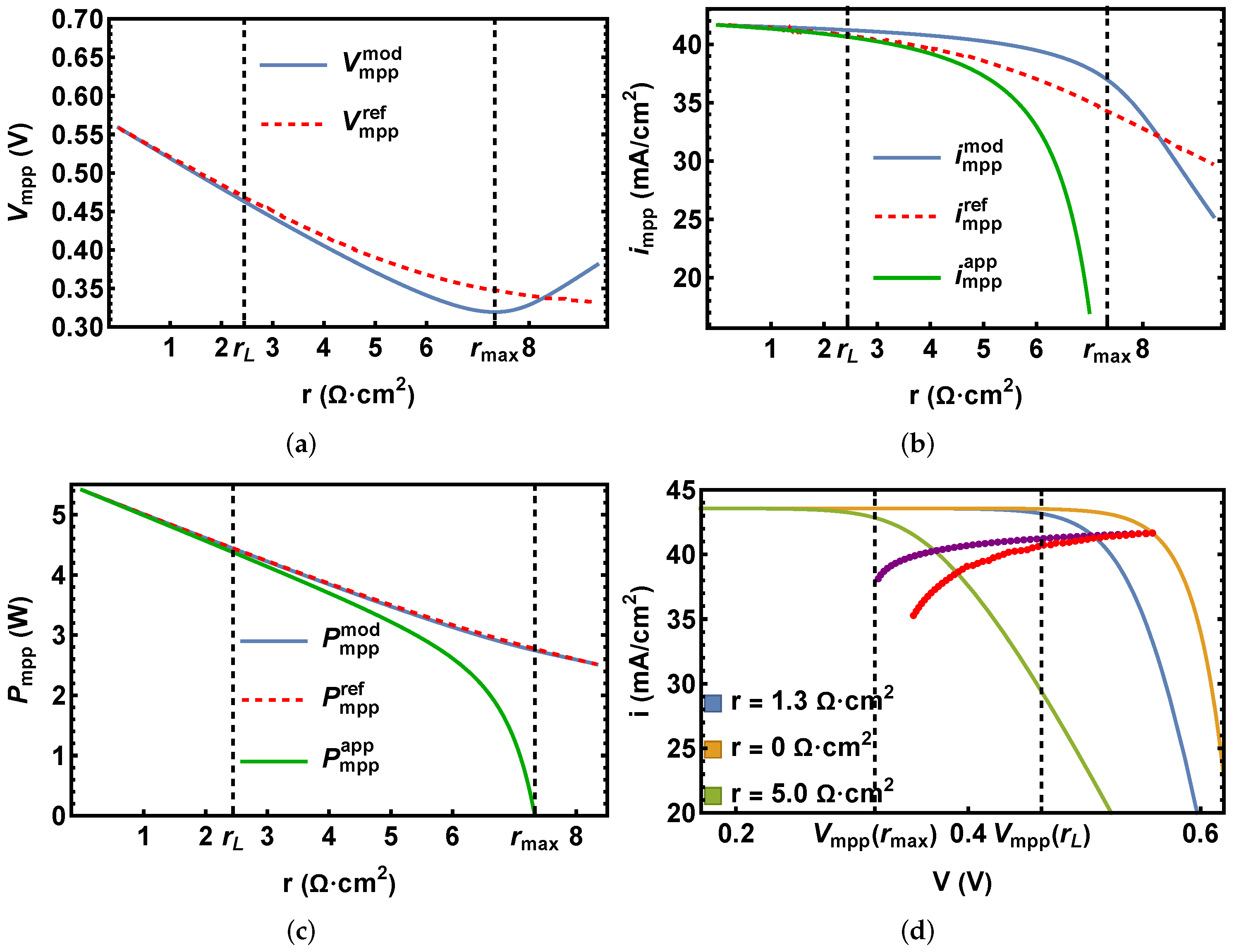
3.1. Maximum Power Point Voltage

The Taylor expansion of the principal branch of Lambert’s W function, ${\mathrm{W}}_0$, is given by:

$${\mathrm{W}}_0\left(x\right)=\sum _{n=1}^{\infty }\frac{{(-n)}^{n-1}}{n!}{x}^n=x-x^2+\frac{3}{2}{x}^3-\frac{8}{3}{x}^4\cdots$$

(9)

which converges as long as $x\le \raisebox{1ex}{$1$}\!\left/ \!\raisebox{-1ex}{$e$}\right.$. The series expansion in Equation (9) can be used to find an approximate analytical solution to Equation (8). To do so, notice that $z_{\mathrm{mpp}}$ may be small for typical solar cells. To see this, note that $i_0$ is given by $i_0\approx qC{V}_{\mathrm{t}}exp\left[-\raisebox{1ex}{$E_g$}\!\left/ \!\raisebox{-1ex}{$q{V}_{\mathrm{t}}$}\right.\right]E_g^2$, where $E_{\mathrm{g}}$ is the bandgap of the semiconductor and C is a constant involving the speed of light, Planck’s constant, and the external radiative efficiency (ERE) [17]. The latter is used to account for nonradiative recombination. $z\left(V\right)$ can then be written as:

$$z\left(V\right)=rC{E}_{\mathrm{g}}^{2}exp\left[\frac{V}{V_{\mathrm{t}}}-\frac{E_{\mathrm{g}}/q}{V_{\mathrm{t}}}+\frac{i_{\mathrm{G}}r}{V_{\mathrm{t}}}\right].$$

(10)

The voltage is limited by the bandgap, and therefore, it holds that $V-\raisebox{1ex}{$E_{\mathrm{g}}$}\!\left/ \!\raisebox{-1ex}{$q$}\right.<0$. As long as the value of r is not excessively large, the exponent in Equation (10) will be negative, resulting in a small z. Assuming a reasonable cell quality, the series expansion in Equation (9) can be used to approximate $\mathrm{W}\left(z_{\mathrm{mpp}}\right)$ by $z_{\mathrm{mpp}}$ in Equation (8). To show this, Figure 1 displays the values of $\mathrm{W}\left(z_{\mathrm{mpp}}\right)$ (continuous lines) and $z_{\mathrm{mpp}}$ (crosses) as a function of the bandgap for various values of r. There, it is confirmed that, for large bandgaps, $\mathrm{W}\left(z_{\mathrm{mpp}}\right)$ is well approximated by $z_{\mathrm{mpp}}$, even for values of r up to $5\Omega ·{\mathrm{cm}}^2$. As expected from Equation (10), Figure 1 shows that the approximation is more accurate for lower values of r. In this context, it is worth noting that typical values for area-normalized series resistance usually are below $2\Omega ·{\mathrm{cm}}^2$ for both laboratory and commercial solar cells [18]. Therefore, $\mathrm{W}\left(z_{\mathrm{mpp}}\right)$ should be well approximated by $z_{\mathrm{mpp}}$ for most solar cells. Figure 1 is obtained assuming an AM1.5G spectrum and ERE value of ${10}^{-4}$. The displayed values correspond to values of $V_{\mathrm{mpp}}$ that were obtained by solving Equation (8) numerically for various values of r and $E_{\mathrm{g}}$.

Figure 1. $\mathrm{W}\left(z_{\mathrm{mpp}}\right)$ (continuous lines) and $z_{\mathrm{mpp}}$ (crosses) as a function of the energy gap, $E_{\mathrm{g}}$, for various values of r. The graph is obtained assuming an AM 1.5G spectrum and ERE = ${10}^{-4}$. The $V_{\mathrm{mpp}}$ values are obtained by solving Equation (8) numerically.

Approximating $\mathrm{W}\left(z_{\mathrm{mpp}}\right)$ by $z_{\mathrm{mpp}}$ in Equation (8) results in:

$$\frac{1}{z_{\mathrm{mpp}}}\frac{V_{\mathrm{G}}}{V_{\mathrm{t}}}=\frac{1+z_{\mathrm{mpp}}+\frac{V_{\mathrm{mpp}}}{V_{\mathrm{t}}}}{1+z_{\mathrm{mpp}}}.$$

(11)

Focusing now on the right-hand side of Equation (11), since $z_{\mathrm{mpp}}$ needs to be small so that the approximation $\mathrm{W}\left(z_{\mathrm{mpp}}\right)\approx z_{\mathrm{mpp}}$ is accurate, the term $\raisebox{1ex}{$V_{\mathrm{mpp}}$}\!\left/ \!\raisebox{-1ex}{$V_{\mathrm{t}}$}\right.$ will dominate over $z_{\mathrm{mpp}}$ in the numerator. Equation (11) can then be simplified to:

$$\frac{1}{z_{\mathrm{mpp}}}\frac{V_{\mathrm{G}}}{V_{\mathrm{t}}}=\frac{1+\frac{V_{\mathrm{mpp}}}{V_{\mathrm{t}}}}{1+z_{\mathrm{mpp}}},$$

(12)

which is analytically solvable. The first step in finding the solution is to insert $z_{\mathrm{mpp}}$. After a bit of manipulation, Equation (12) becomes:

$$\begin{array}{c}\hfill \left(1+\frac{V_{\mathrm{mpp}}-V_{\mathrm{G}}}{V_{\mathrm{t}}}\right)exp\left[1+\frac{V_{\mathrm{mpp}}-V_{\mathrm{G}}}{V_{\mathrm{t}}}\right]=\frac{V_{\mathrm{G}}}{V_0}exp\left[1-2\frac{V_{\mathrm{G}}}{V_{\mathrm{t}}}\right],\end{array}$$

(13)

which has the closed-form solution:

$$V_{\mathrm{mpp}}=V_{\mathrm{G}}+V_{\mathrm{t}}\left(\mathrm{W}\left[\frac{V_{\mathrm{G}}}{V_0}exp\left[1-2\frac{V_{\mathrm{G}}}{V_{\mathrm{t}}}\right]\right]-1\right).$$

(14)

Finally, inserting the definitions for $V_{\mathrm{G}}$ and $V_0$ yields:

$$V_{\mathrm{mpp}}=i_{\mathrm{G}}r+V_{\mathrm{t}}\left(\mathrm{W}\left[\frac{i_{\mathrm{G}}}{i_0}exp\left[1-2\frac{i_{\mathrm{G}}r}{V_{\mathrm{t}}}\right]\right]-1\right),$$

(15)

from which it can be seen that, in the limit $r\to 0$, Equation (15) becomes Equation (3).

3.2. Maximum Power Point Current and Power

In order to obtain expressions for $i_{\mathrm{mpp}}$ and $P_{\mathrm{mpp}}$, Equation (15) has to be inserted into Equation (7). This results in a composite of W functions that cannot be simplified. A simpler approximate expression for $i_{\mathrm{mpp}}$ can be obtained by noting that at the maximum power point, the W function in Equation (7) is evaluated at $z\left(V\right)=z_{\mathrm{mpp}}$. Since $z_{\mathrm{mpp}}$ needs to be small for Equation (15) to be accurate, $\mathrm{W}\left(z_{\mathrm{mpp}}\right)$ can be approximated by $z_{\mathrm{mpp}}$ here as well. From Equation (7), this yields:

$$\begin{array}{cc}\hfill i_{\mathrm{mpp}}=i_{\mathrm{G}}-\frac{V_{\mathrm{t}}}{r}\mathrm{W}\left(z_{\mathrm{mpp}}\right)& \approx i_{\mathrm{G}}-\frac{V_{\mathrm{t}}}{r}{z}_{\mathrm{mpp}}\hfill \\ \hfill & =i_{\mathrm{G}}-i_{0}exp\left[\frac{V_{\mathrm{mpp}}}{V_{\mathrm{t}}}+\frac{V_{\mathrm{G}}}{V_{\mathrm{t}}}\right].\hfill \end{array}$$

(16)

An analytical expression for $i_{\mathrm{mpp}}$ can now be obtained by inserting Equation (15) into (16), and an analytical expression for $P_{\mathrm{mpp}}$ can be found by evaluating $V_{\mathrm{mpp}}·i_{\mathrm{mpp}}$. To shorten the notation, let $\alpha \left(r\right)$ denote the argument of the W function in Equation (15). The approximate analytical expressions for $i_{\mathrm{mpp}}$ and $P_{\mathrm{mpp}}$ then become:

$$\begin{array}{cc}\hfill i_{\mathrm{mpp}}=& i_{\mathrm{G}}\left(1-\frac{1}{\mathrm{W}\left[\alpha \left(r\right)\right]}\right),\hfill \end{array}$$

(17)

$$\begin{array}{cc}\hfill P_{\mathrm{mpp}}=& i_{\mathrm{G}}^{2}r\left(1-\frac{1}{\mathrm{W}\left[\alpha \left(r\right)\right]}\right)+i_{\mathrm{G}}{V}_{\mathrm{t}}\left(\mathrm{W}\left[\alpha \left(r\right)\right]-2+\frac{1}{\mathrm{W}\left[\alpha \left(r\right)\right]}\right).\hfill \end{array}$$

(18)

Note that in the limit $r\to 0$, Equations (4) and (5) are recovered.

3.3. Practical Note

For practical applications of Equations (15), (17) and (18), it is worth noting that $i_{\mathrm{G}}$ is well approximated by $i_{\mathrm{sc}}$, even though the latter is dependent on the series resistance. In the case of, e.g., silicon under an AM 1.5 G spectrum, $i_{\mathrm{G}}$ and $i_{\mathrm{sc}}$ practically overlap for values of r up to about $11\Omega ·{\mathrm{cm}}^2$. Additionally, note that the quotient $\raisebox{1ex}{$i_{\mathrm{sc}}$}\!\left/ \!\raisebox{-1ex}{$i_0$}\right.$ can be expressed as $exp\left(\raisebox{1ex}{$V_{\mathrm{oc}}$}\!\left/ \!\raisebox{-1ex}{$V_{\mathrm{t}}$}\right.\right)$. Equation (15) then becomes:

$$V_{\mathrm{mpp}}=i_{\mathrm{sc}}r+V_{\mathrm{t}}\left(\mathrm{W}\left[exp\left[1+\frac{V_{\mathrm{oc}}}{V_{\mathrm{t}}}-2\frac{i_{\mathrm{sc}}r}{V_{\mathrm{t}}}\right]\right]-1\right).$$

(19)

These practical substitutions may be also applied to Equations (17) and (18).

4. Analytical Expression for the Series Resistance

From Equation (19), it is possible to obtain r as a function of $V_{\mathrm{mpp}}$. To see this, note that Equation (19) can be rewritten as:

$$1+\frac{V_{\mathrm{mpp}}-i_{\mathrm{sc}}r}{V_{\mathrm{t}}}=\mathrm{W}\left[exp\left[1+\frac{V_{\mathrm{oc}}}{V_{\mathrm{t}}}-2\frac{i_{\mathrm{sc}}r}{V_{\mathrm{t}}}\right]\right],$$

(20)

which is equivalent to:

$$\begin{array}{c}\hfill \left(1+\frac{V_{\mathrm{mpp}}-i_{\mathrm{sc}}r}{V_{\mathrm{t}}}\right)exp\left[1+\frac{V_{\mathrm{mpp}}-i_{\mathrm{sc}}r}{V_{\mathrm{t}}}\right]=exp\left[1+\frac{V_{\mathrm{oc}}}{V_{\mathrm{t}}}-2\frac{i_{\mathrm{sc}}r}{V_{\mathrm{t}}}\right],\end{array}$$

(21)

which is seen by applying Lambert’s W function to both sides of Equation (21) and using the definition $x=\mathrm{W}\left(x{e}^x\right)$. Multiplying both sides by $exp\left[-2\raisebox{1ex}{$V_{\mathrm{mpp}}$}\!\left/ \!\raisebox{-1ex}{$V_{\mathrm{t}}$}\right.+2\raisebox{1ex}{$i_{\mathrm{sc}}r$}\!\left/ \!\raisebox{-1ex}{$V_{\mathrm{t}}$}\right.\right]$ yields:

$$\begin{array}{c}\hfill exp\left[1+\frac{V_{\mathrm{oc}}}{V_{\mathrm{t}}}-2\frac{V_{\mathrm{mpp}}}{V_{\mathrm{t}}}\right]=\left(1+\frac{V_{\mathrm{mpp}}-i_{\mathrm{sc}}r}{V_{\mathrm{t}}}\right)exp\left[1-\frac{V_{\mathrm{mpp}}-i_{\mathrm{sc}}r}{V_{\mathrm{t}}}\right].\end{array}$$

(22)

Finally, multiplying both sides by $-e^{-2}$ gives:

$$\begin{array}{c}\hfill -exp\left[-1+\frac{V_{\mathrm{oc}}}{V_{\mathrm{t}}}-2\frac{V_{\mathrm{mpp}}}{V_{\mathrm{t}}}\right]=\left(-1-\frac{V_{\mathrm{mpp}}-i_{\mathrm{sc}}r}{V_{\mathrm{t}}}\right)exp\left[-1-\frac{V_{\mathrm{mpp}}-i_{\mathrm{sc}}r}{V_{\mathrm{t}}}\right],\end{array}$$

(23)

which can be inverted by making use of Lambert’s W function. After some manipulation, r can be expressed as:

$$r=\frac{V_{\mathrm{mpp}}}{i_{\mathrm{sc}}}+\frac{V_{\mathrm{t}}}{i_{\mathrm{sc}}}\left(\mathrm{W}\left[-exp\left[-1+\frac{V_{\mathrm{oc}}}{V_{\mathrm{t}}}-2\frac{V_{\mathrm{mpp}}}{V_{\mathrm{t}}}\right]\right]+1\right).$$

(24)

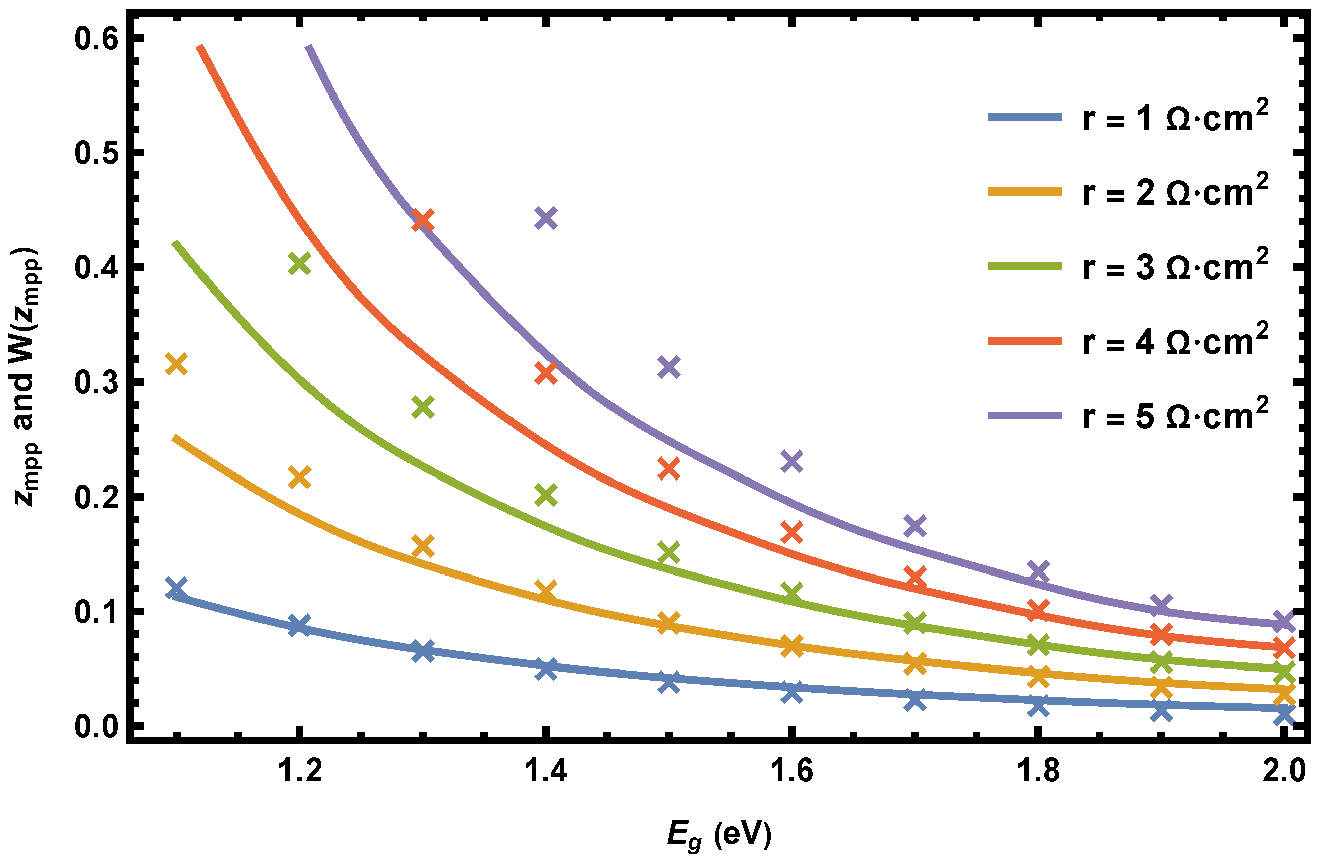
4.1. Validity of the Approximate Expression

Equation (24) sets the limit for the range of r where Equation (19) describes the physical behavior of $V_{\mathrm{mpp}}$. As the exponential function only yields positive values, the argument of Lambert’s W in Equation (24) is negative. The principal branch of Lambert’s W function, ${\mathrm{W}}_0\left(z\right)$, is only defined for $z\ge -\raisebox{1ex}{$1$}\!\left/ \!\raisebox{-1ex}{$e$}\right.$, which implies that $\mathrm{W}\left(z\right)\notin \mathcal{R}$ for $z\le -\raisebox{1ex}{$1$}\!\left/ \!\raisebox{-1ex}{$e$}\right.$. Since the series resistance is a real-valued physical quantity, the argument of the W function in Equation (24) must fulfill:

$$exp\left[-1+\frac{V_{\mathrm{oc}}}{V_{\mathrm{t}}}-2\frac{V_{\mathrm{mpp}}}{V_{\mathrm{t}}}\right]\le \frac{1}{e},$$

(25)

which implies:

$$V_{\mathrm{mpp}}\ge \frac{1}{2}{V}_{\mathrm{oc}}.$$

(26)

Equation (26) sets an upper limit for the series resistance, as having $V_{\mathrm{mpp}}$ less than $\frac{1}{2}{V}_{\mathrm{oc}}$ would require a complex-valued r. This translates into Equation (15) not describing a physical $V_{\mathrm{mpp}}$ for any value of the series resistance, which would make $V_{\mathrm{mpp}}$ smaller than $\raisebox{1ex}{$V_{\mathrm{oc}}$}\!\left/ \!\raisebox{-1ex}{$2$}\right.$. This maximum value of the resistance, which is denoted in the present work by $r_{\max }$, is found by evaluating Equation (24) at $V_{\mathrm{mpp}}=\raisebox{1ex}{$V_{\mathrm{oc}}$}\!\left/ \!\raisebox{-1ex}{$2$}\right.$. This yields:

$$r_{\max }=r\left[\frac{V_{\mathrm{oc}}}{2}\right]=\frac{V_{\mathrm{oc}}/2}{i_{\mathrm{sc}}}+\frac{V_{\mathrm{t}}}{i_{\mathrm{sc}}}\left(\mathrm{W}\left[-\frac{1}{e}\right]+1\right)=\frac{V_{\mathrm{oc}}}{2i_{\mathrm{sc}}}.$$

Note that at $r=r_{\max }$, the parentheses in Equation (19) cancel out. For $r\ge r_{\max }$, the W function tends asymptotically to zero. This results in $V_{\mathrm{mpp}}$ increasing linearly with r with slope $i_{\mathrm{sc}}$, which is not physical.

4.2. Accuracy of the Approximation

The accuracy of Equation (15) decreases with increasing series resistance. For sufficiently large r, the term involving $z_{\mathrm{mpp}}$ in the numerator on the right-hand side of Equation (11) will not be small in comparison to $\raisebox{1ex}{$V_{\mathrm{mpp}}$}\!\left/ \!\raisebox{-1ex}{$V_{\mathrm{t}}$}\right.$, implying that Equation (15) will be less accurate. Therefore, it is relevant to determine the value of the series resistance, $r_{\mathrm{L}}$, until the derived model gives the acceptable results. The value $r_{\mathrm{L}}=\raisebox{1ex}{$r_{\max }$}\!\left/ \!\raisebox{-1ex}{$3$}\right.$ is proposed as a rule of thumb. This corresponds roughly to $z_{\mathrm{mpp}}\approx \raisebox{1ex}{$1$}\!\left/ \!\raisebox{-1ex}{$e$}\right.$, which seems a natural choice since for $z_{\mathrm{mpp}}\ge \raisebox{1ex}{$1$}\!\left/ \!\raisebox{-1ex}{$e$}\right.$, the Taylor expansion in Equation (9) should not be applicable as $z_{\mathrm{mpp}}$ would be larger than the convergence radius of the expansion. Determining the actual value of r that makes $z_{\mathrm{mpp}}=\raisebox{1ex}{$1$}\!\left/ \!\raisebox{-1ex}{$e$}\right.$ would require solving simultaneously $z_{\mathrm{mpp}}-\raisebox{1ex}{$1$}\!\left/ \!\raisebox{-1ex}{$e$}\right.=0$ and Equation (8), which is rather counterproductive, since the main point of making use of Equation (15) is to avoid solving Equation (8) numerically.

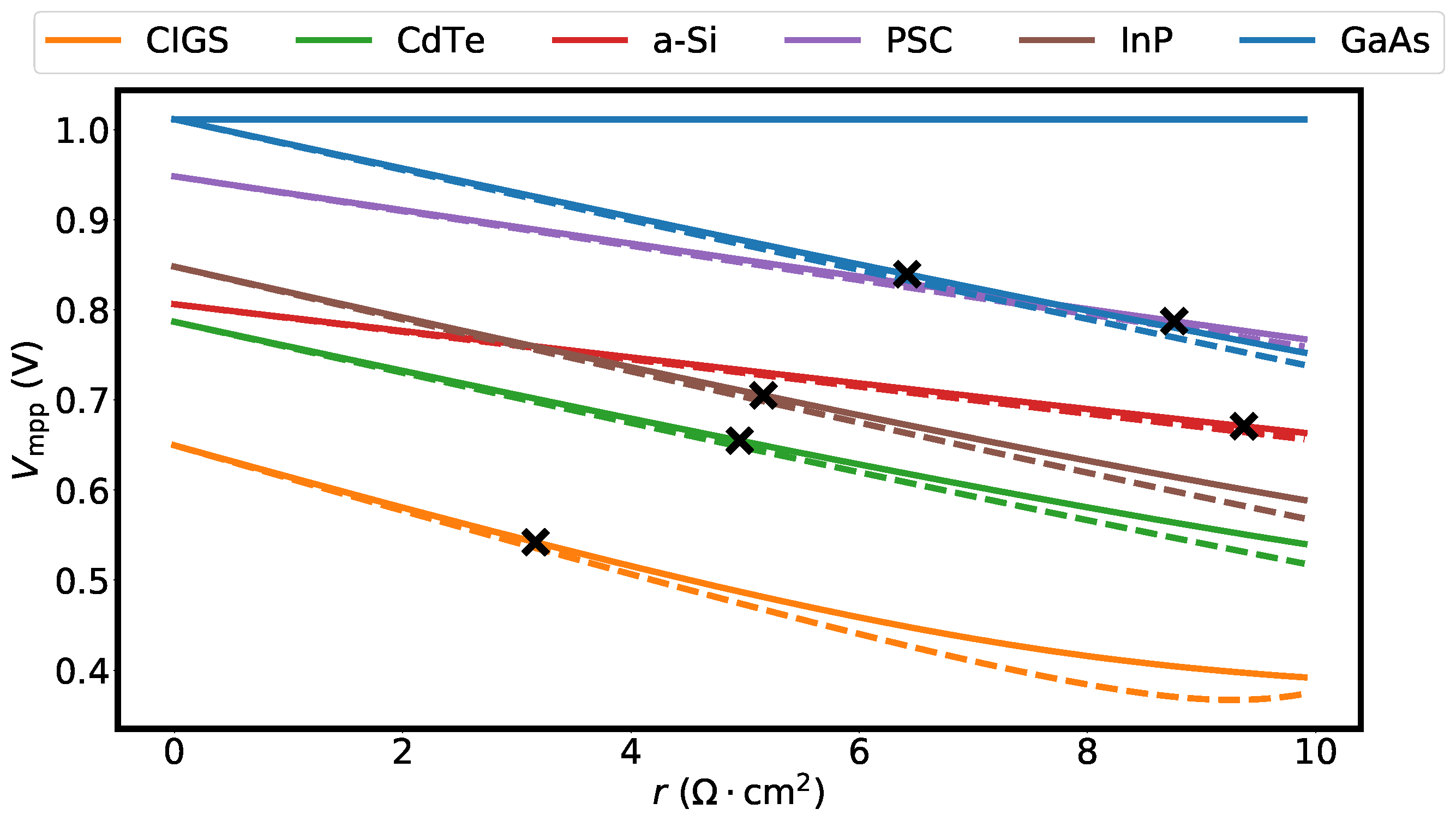
5. Numerical Results

In this section, the accuracy of Equation (19) is tested. For this, the focus is on $V_{\mathrm{mpp}}$ and $P_{\mathrm{mpp}}$, given by $P_{\mathrm{mpp}}=V_{\mathrm{mpp}}i\left(V_{\mathrm{mpp}}\right)$, with i being given by Equation (7). The label “mod” is used to denote the values of $V_{\mathrm{mpp}}$ and $P_{\mathrm{mpp}}$ obtained from Equation (19). The label “ref” is used to denote the reference values to which $V_{\mathrm{mpp}}^{\mathrm{mod}}$ and $P_{\mathrm{mpp}}^{\mathrm{mod}}$ are compared. The “ref” quantities are obtained by numerically solving Equation (8). The accuracy of Equations (17) and (18) is also tested, and the label “app” is used to denote these.

For all numerical calculations, the AM 1.5G spectrum was assumed. The numerical single-diode model used to test the accuracy of Equation (19) was fed with cell parameters corresponding to six different technologies found in the latest installment of the solar cell efficiency tables [19]. The parameters corresponding to these cells are summarized in Table 1. As a seventh case, the derived model was also tested against a numerical single-diode model using $E_{\mathrm{g}}=1.125$ eV and $\mathrm{ERE}={10}^{-4}$. These values are typical for silicon cells. This case is therefore referred to as a numerically modeled silicon cell. All cells were assumed to be at a temperature of 300 K. Figure 2 displays (a) $V_{\mathrm{mpp}}$, (b) $i_{\mathrm{mpp}}$, and (c) $P_{\mathrm{mpp}}$ as a function of the series resistance. Additionally, the corresponding current–voltage characteristic (Figure 2d) is shown for several values of the series resistance. All curves correspond to the numerically modeled silicon cell described above. In Figure 2d, dotted lines show how the maximum power point changes with increasing series resistance. The red dotted line was obtained by solving Equation (8) numerically, for multiple values of the series resistance, and evaluating Equation (7) with the obtained $V_{\mathrm{mpp}}$ values. The purple dotted line was obtained from Equation (15). The values for $r_{\mathrm{L}}$ and $r_{\max }$ (Figure 2a–c) and their correspondent values of $V_{\mathrm{mpp}}$ (Figure 2d) are displayed with black vertical dashed lines. From Figure 2a–c, it can be seen that the values calculated with the new analytical model were in good agreement with the numerical reference model for $r\le r_{\mathrm{L}}$. For $r\ge r_{\mathrm{L}}$, $V_{\mathrm{mpp}}^{\mathrm{mod}}$ appears to be underestimated (Figure 2a) and $i_{\mathrm{mpp}}^{\mathrm{mod}}$ overestimated (Figure 2b). As a result, $P_{\mathrm{mpp}}^{\mathrm{mod}}$ overlaps well with $P_{\mathrm{mpp}}^{\mathrm{ref}}$ (Figure 2c). Finally, for $r\ge r_{\max }$, $V_{\mathrm{mpp}}^{\mathrm{mod}}$ appears to increase with increasing series resistance.

Table 1. Parameters for selected single-junction solar cell technologies. The ERE values were estimated from Equation (27).

Device	$E_{\mathrm{g}}\left(\mathrm{eV}\right)$	$V_{\mathrm{oc}}$ (V) 1	$i_{\mathrm{sc}}$$(\mathrm{mA}/{\mathrm{cm}}^2)$1	ERE $(\%)$
InP	1.34	0.939	31.15	0.365
GaAs	1.42	1.107	29.60	14.510
CdTe	1.51	0.876	30.25	${10}^{-4}$
CIGS	1.08	0.734	39.58	1.750
a-Si	1.69	0.896	16.36	1.96 $\times {10}^{-7}$
PSC 2	1.60	1.042	20.40	0.002

¹ The $V_{\mathrm{oc}}$ and $i_{\mathrm{sc}}$ values were measured under the AM 1.5 G spectrum at T = 300 K [19]. ² Perovskite solar cell.

Figure 2. $V_{\mathrm{mpp}}$ (a), $i_{\mathrm{mpp}}$ (b), and $P_{\mathrm{mpp}}$ (c) as a function of the series resistance. For (c), a typical Si solar cell size of $6\times 6{\mathrm{inch}}^2$ ($0.0232{\mathrm{m}}^2$) was assumed. (d) Current–voltage characteristics for three different values of series resistance. The dotted lines (Equation (15) in purple and Equation (8) in red) represent the maximum power point changing with increasing series resistance.

The accuracy of the expression for $V_{\mathrm{mpp}}^{\mathrm{mod}}$, Equation (19), decreases with increasing resistance. This can be seen in Figure 3, where $V_{\mathrm{mpp}}$ is plotted as a function of the series resistance for the six technologies presented in Table 1. The dashed lines correspond to the reference values, $V_{\mathrm{mpp}}^{\mathrm{ref}}$ and the continuous lines to $V_{\mathrm{mpp}}^{\mathrm{mod}}$. The points corresponding to a series resistance equal to $r_{\mathrm{L}}$ are marked with crosses. Focusing on the graphs representing the CIGS cell, the mismatch between $V_{\mathrm{mpp}}^{\mathrm{ref}}$ and $V_{\mathrm{mpp}}^{\mathrm{mod}}$ becomes noticeable for $r\ge r_{\mathrm{L}}$. For additional comparison, the $V_{\mathrm{mpp}}$ calculated from Equation (3) (i.e., without series resistance) for the GaAs cell is displayed in Figure 3. This is represented by the blue straight line with zero slope. At $r=0\Omega ·{\mathrm{cm}}^2$, $V_{\mathrm{mpp}}^{\mathrm{ref}}$, $V_{\mathrm{mpp}}^{\mathrm{mod}}$, and Equation (3) overlap, but as soon as r starts increasing, Equation (19) predicts the value of $V_{\mathrm{mpp}}^{\mathrm{ref}}$ with higher accuracy. Finally, it is worth mentioning that the overlap between $V_{\mathrm{mpp}}^{\mathrm{mod}}$ and $V_{\mathrm{mpp}}^{\mathrm{ref}}$ is particularly good with the perovskite (PSC) and the amorphous silicon (a-Si) solar cells due to their large bandgaps. Table 2 displays the values of $V_{\mathrm{mpp}}$ and $P_{\mathrm{mpp}}$ corresponding to the numerically modeled Si cell shown in Figure 2 for various values of the series resistance. From the left, the first column presents five values of area-normalized series resistance. In the second column, the values of $V_{\mathrm{mpp}}^{\mathrm{mod}}$ and $V_{\mathrm{mpp}}^{\mathrm{ref}}$ are presented, followed by their relative discrepancy in %. The three remaining columns follow the same structure, but with the values of $P_{\mathrm{mpp}}^{\mathrm{mod}}$ and $P_{\mathrm{mpp}}^{\mathrm{ref}}$. Table 2 shows that the higher the series resistance, the higher the discrepancy is. Nevertheless, the model derived in the present work has a reasonable accuracy and is able to predict the value of $P_{\mathrm{mpp}}$ with an error below $0.75\%$ for series resistance up to $5\Omega ·{\mathrm{cm}}^2$ for this numerically modeled cell.

Figure 3. $V_{\mathrm{mpp}}$ as a function of the series resistance at T = 300 K. $V_{\mathrm{mpp}}^{\mathrm{mod}}$ (Equation (15)) is represented by continuous lines and $V_{\mathrm{mpp}}^{\mathrm{ref}}$ (Equation (8)) by dashed lines.

Table 2. Comparison of $V_{\mathrm{mpp}}$ and $P_{\mathrm{mpp}}$ for various values of area-normalized series resistance. The values correspond to a numerically modeled Si cell ($E_{\mathrm{g}}=1.125$ eV) with ERE = ${10}^{-4}$ at T = 300 K.

r$(\Omega ·{\mathrm{cm}}^2)$	$V_{\mathrm{mpp}}$ (V)		Error $(\%)$	$P_{\mathrm{mpp}}$ (W)		Error $(\%)$
	$V_{\mathrm{mpp}}^{\mathrm{mod}}$	$V_{\mathrm{mpp}}^{\mathrm{ref}}$		$P_{\mathrm{mpp}}^{\mathrm{mod}}$	$P_{\mathrm{mpp}}^{\mathrm{ref}}$
0	0.559	0.559	${10}^{-4}$	5.414	5.414	${10}^{-8}$
0.5	0.539	0.540	0.153	5.213	5.213	0.003
1.5	0.500	0.503	0.629	4.813	4.815	0.034
2.0	0.480	0.485	1.032	4.615	4.618	0.066
5.0	0.371	0.390	4.906	3.477	3.502	0.728

Figure 4 displays the base-10 logarithm of the relative discrepancy (in %) between $P_{\mathrm{mpp}}^{\mathrm{mod}}$ and $P_{\mathrm{mpp}}^{\mathrm{ref}}$ as a function of the bandgap energy and the ERE for $r=2\Omega ·{\mathrm{cm}}^2$. The relative discrepancy between $P_{\mathrm{mpp}}^{\mathrm{mod}}$ and $P_{\mathrm{mpp}}^{\mathrm{ref}}$ for the six solar cell technologies presented in Table 1 is also shown. The white dotted lines represent levels of fixed relative discrepancy. To compute this figure, the ERE values of the solar cells presented in Table 1 were estimated by making use of:

$$\mathrm{ERE}=exp\left[\frac{V_{\mathrm{oc}}-V_{\mathrm{oc}}^{\mathrm{rad}}}{V_{\mathrm{t}}}\right],$$

(27)

where $V_{\mathrm{oc}}^{\mathrm{rad}}$ can be calculated from Equation (1) by assuming that $i_0$ results only from radiative recombination. Figure 4 shows that, for a given series resistance, the accuracy of Equation (15) increases with increasing bandgap and decreases with decreasing ERE. Note that the $P_{\mathrm{mpp}}$ of all the investigated cases was predicted with a discrepancy below $0.07\%$. Finally, Figure 5 displays the base-10 logarithm of the relative discrepancy (in %) between $P_{\mathrm{mpp}}^{\mathrm{ref}}$ and $P_{\mathrm{mpp}}^{\mathrm{mod}}$ (Figure 5a) and between $P_{\mathrm{mpp}}^{\mathrm{ref}}$ and $P_{\mathrm{mpp}}^{\mathrm{app}}$ (Figure 5b) as a function of the series resistance for the six devices presented in Table 1. Here, it can be seen that the discrepancy between $P_{\mathrm{mpp}}^{\mathrm{ref}}$ and $P_{\mathrm{mpp}}^{\mathrm{app}}$ is around one order of magnitude larger than between $P_{\mathrm{mpp}}^{\mathrm{mod}}$ and $P_{\mathrm{mpp}}^{\mathrm{ref}}$. $P_{\mathrm{mpp}}^{\mathrm{app}}$ could still predict $P_{\mathrm{mpp}}$ in most of the studied cases with errors below 1% for values of the series resistance up to 5 $\Omega ·{\mathrm{cm}}^2$.

Figure 4. Logarithm of the relative discrepancy (in %) between $P_{\mathrm{mpp}}^{\mathrm{mod}}$ (Equation (15)) and $P_{\mathrm{mpp}}^{\mathrm{ref}}$ (Equation (8)) as a function of the bandgap energy and the ERE at T = 300 K and $r=2\Omega ·{\mathrm{cm}}^2$. The small bends in the dashed lines originated from the irregular shape of the AM 1.5G spectrum.

Figure 5. Logarithm of the relative discrepancy (in %) between (a) $P_{\mathrm{mpp}}^{\mathrm{ref}}$ (Equation (8)) and $P_{\mathrm{mpp}}^{\mathrm{mod}}$ (Equation (15)) and (b) $P_{\mathrm{mpp}}^{\mathrm{ref}}$ and $P_{\mathrm{mpp}}^{\mathrm{app}}$ (Equation (18)) as a function of the series resistance at T = 300 K.

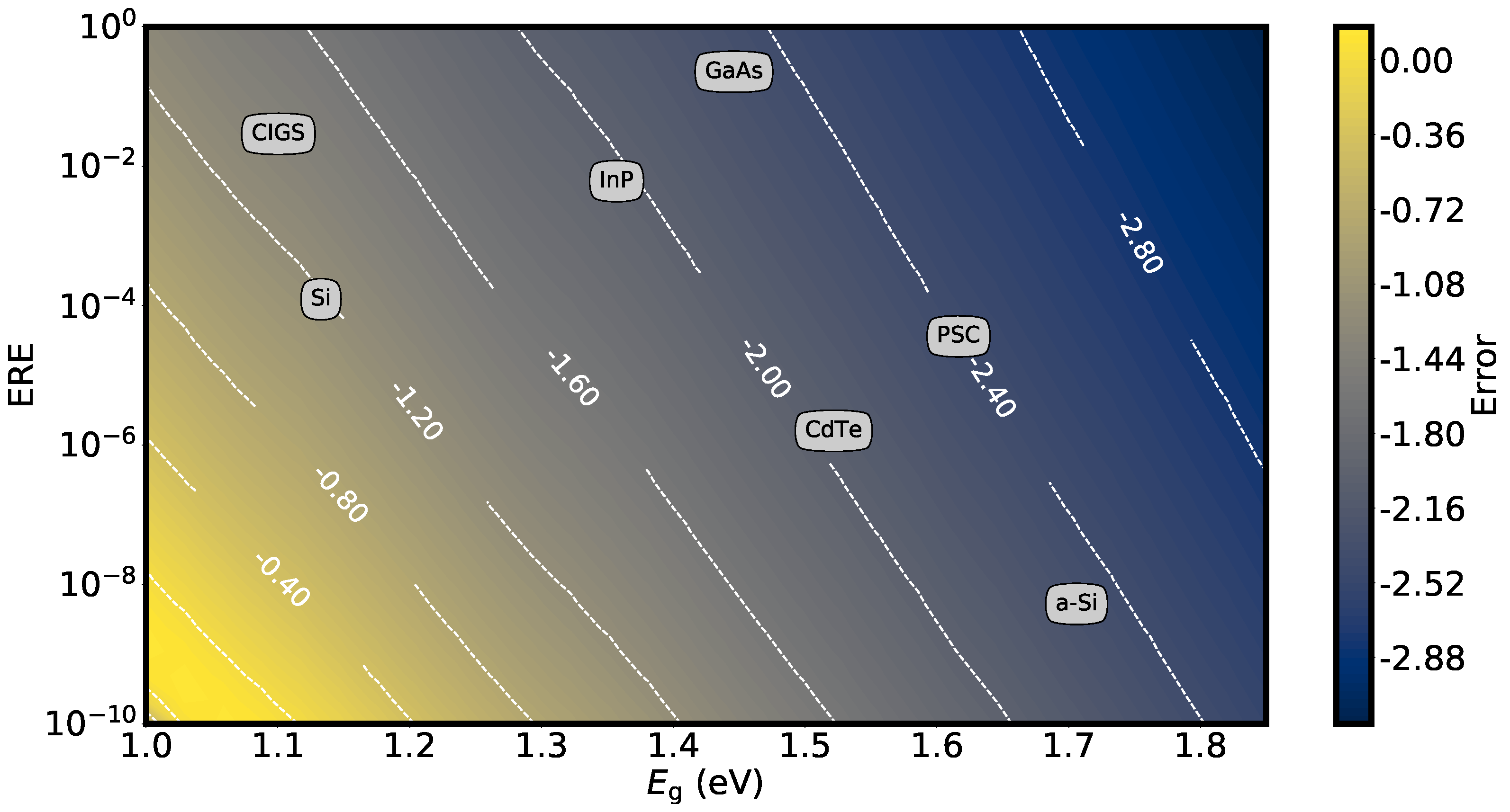
6. Experimental Validation and Remarks

Now that the analytical model has been numerically validated, its applicability in real cells should be tested. This was performed in [10], where 18 multicrystalline silicon solar cells with different bulk resistivities and cell architectures were measured at multiple temperatures. For the studied cells, Equations (18) and (19) predicted the experimental $P_{\mathrm{mpp}}$ and $V_{\mathrm{mpp}}$ with relative discrepancies below $0.2\%$ and $0.7\%$, respectively. It is worth mentioning that low relative discrepancies were obtained at all the measured temperatures.

Besides the numerical limitations that the model derived in the present work may have (e.g., Equation (26)), practical limitations of the model should be addressed. These may include factors that real cells will eventually experience, for instance, degradation due to aging or shunt resistance effects. Although the derived model cannot account for, e.g., cell degradation, it is worth noting that neither can the diode equation in Equation (1), nor the modified diode equation in Equation (6). The analytical expressions derived in the present work were subjected to the same practical limitations that the modified diode equation was. The advantage that the derived model presents with respect to Equation (6) is that it allows seeing how the series resistance affects the MPP analytically. On the other hand, shunt resistance effects do not usually have a relevant impact in laboratory cells, as these typically appear due to defects in manufacturing. In fact, in [10], the shunt resistance in the measured cells had only a negligible effect on the comparison between the model and the experiments. Although it might be possible to obtain an expression analogous to Equation (19) that also accounts for the effect of shunt resistance, this goes beyond the scope of the present work.

7. Conclusions

In this work, a new analytical expression for the maximum power point voltage that explicitly accounts for the effect of the series resistance was derived. Approximate analytical expressions for the current and power at the maximum power point were also presented. To derive these expressions, it was shown that Lambert’s W function may be approximated by its argument, as long as the value of the series resistances is not excessively large. This makes what otherwise would be a transcendental problem analytically solvable. The accuracy of the new expressions was tested with a numerical single-diode model. It was shown that the new model accurately predicts the maximum power of all the investigated cases with small discrepancies between the analytical model and the numerically simulated values. This was the case even when considering values of the series resistance above $2\Omega ·{\mathrm{cm}}^2$, which is larger than typical values for laboratory and commercial cells [18]. The accuracy of the approximation was shown to decrease with increasing series resistance, but also to increase with increasing bandgap energy. This makes the derived model of particular interest for semiconductors with large bandgaps such as perovskite or organic solar cells. Based on the results presented in this work, together with the results published in [10], it may be concluded that the derived analytical model can successfully be utilized to predict the maximum power point for solar cells that follow the diode equation when series resistance is accounted for. Moreover, the employment of Lambert’s W function allowed for accurate and simpler expressions than what is currently found in the scientific literature. With respect to new developments, the derived model opens the possibility of analytically studying the effect of the series resistance on the temperature coefficients of the maximum power point. Further enhancements may also include attempts to generalize the model derived in the present work to also include the effect of the shunt resistance.

References

- Shockley, W.; Queisser, H.J. Detailed balance limit of efficiency of p-n junction solar cells. J. Appl. Phys. 1961, 32, 510–519. [Google Scholar] [CrossRef]
- Banwell, T.C.; Jayakumar, A. Exact analytical solution for current flow through diode with series resistance. Electron. Lett. 2000, 36, 291–292. [Google Scholar] [CrossRef]
- Jain, A.; Kapoor, A. Exact analytical solutions of the parameters of real solar cells using Lambert W-function. Sol. Energy Mater. Sol. Cells 2004, 81, 269–277. [Google Scholar] [CrossRef]
- Singal, C.M. Analytical expression for the series-resistance-dependent maximum power point and curve factor for solar cells. Sol. Cells 1981, 3, 163–177. [Google Scholar] [CrossRef]
- Green, M.A. Accurate expressions for solar cell fill factors including series and shunt resistances. Appl. Phys. Lett. 2016, 108, 081111. [Google Scholar] [CrossRef]
- Arjun, M.; Ramana, V.V.; Viswadev, R.; Venkatesaperumal, B. An iterative analytical solution for calculating maximum power point in photovoltaic systems under partial shading conditions. IEEE Trans. Circuits Syst. II Express Briefs 2018, 66, 973–977. [Google Scholar] [CrossRef]
- Laudani, A.; Lozito, G.M.; Lucaferri, V.; Radicioni, M.; Fulginei, F.R.; Salvini, A.; Coco, S. An analytical approach for maximum power point calculation for photovoltaic system. In Proceedings of the 2017 European Conference on Circuit Theory and Design (ECCTD), Catania, Italy, 4–6 September 2017; IEEE: New York, NY, USA, 2017; pp. 1–4. [Google Scholar]
- Xenophontos, A.; Bazzi, A.M. Model-based maximum power curves of solar photovoltaic panels under partial shading conditions. IEEE J. Photovoltaics 2017, 8, 233–238. [Google Scholar] [CrossRef]
- Ramadan, A.; Kamel, S.; Taha, I.; Tostado-Véliz, M. Parameter Estimation of Modified Double-Diode and Triple-Diode Photovoltaic Models Based on Wild Horse Optimizer. Electronics 2021, 10, 2308. [Google Scholar] [CrossRef]
- Garcia, A.S.; Kristensen, S.T.; Strandberg, R. Assessment of a New Analytical Expression for the Maximum-Power Point Voltage with Series Resistance. In Proceedings of the 2021 IEEE 48th Photovoltaic Specialists Conference (PVSC), Fort Lauderdale, FL, USA, 20–25 June 2021; IEEE: New York, NY, USA, 2021; pp. 0961–0965. [Google Scholar]
- Shockley, W. The Theory of p-n Junctions in Semiconductors and p-n Junction Transistors. Bell Syst. Tech. J. 1949, 28, 435–489. [Google Scholar] [CrossRef]
- Cuevas, A. The recombination parameter J0. Energy Procedia 2014, 55, 53–62. [Google Scholar] [CrossRef] [Green Version]
- Nelson, J. The Physics of Solar Cells; World Scientific Publishing Company: Singapore, 2003. [Google Scholar]
- Khanna, A.; Mueller, T.; Stangl, R.A.; Hoex, B.; Basu, P.K.; Aberle, A.G. A fill factor loss analysis method for silicon wafer solar cells. IEEE J. Photovoltaics 2013, 3, 1170–1177. [Google Scholar] [CrossRef]
- Sergeev, A.; Sablon, K. Exact solution, endoreversible thermodynamics, and kinetics of the generalized Shockley-Queisser model. Phys. Rev. Appl. 2018, 10, 064001. [Google Scholar] [CrossRef] [Green Version]
- Corless, R.M.; Gonnet, G.H.; Hare, D.E.G.; Jeffrey, D.J.; Knuth, D.E. On the Lambert W function. Adv. Comput. Math. 1996, 5, 329–359. [Google Scholar] [CrossRef]
- Green, M.A. Radiative efficiency of state-of-the-art photovoltaic cells. Prog. Photovoltaics Res. Appl. 2012, 20, 472–476. [Google Scholar] [CrossRef]
- Honsberg, C.B.; Bowden, S.G. Series Resistance. 2019. Available online: https://www.pveducation.org/pvcdrom/solar-cell-operation/series-resistance (accessed on 19 March 2021).
- Green, M.A.; Emery, K.; Hishikawa, Y.; Warta, W.; Dunlop, E.D.; Levi, D.H.; Ho-Baillie, A.W.Y. Solar cell efficiency tables (version 57). Prog. Photovoltaics Res. Appl. 2017, 25, 3–13. [Google Scholar] [CrossRef]
Publisher’s Note: MDPI stays neutral with regard to jurisdictional claims in published maps and institutional affiliations. |
© 2021 by the authors. Licensee MDPI, Basel, Switzerland. This article is an open access article distributed under the terms and conditions of the Creative Commons Attribution (CC BY) license (https://creativecommons.org/licenses/by/4.0/).