Demodulation of EM Telemetry Data Using Fuzzy Wavelet Neural Network with Logistic Response

Abstract

Data telemetry is a critical element of successful unconventional well drilling operations, involving the transmission of information about the well-surrounding geology to the surface in real-time to serve as the basis for geosteering and well planning. However, the data extraction and code recovery (demodulation) process can be a complicated system due to the non-linear and time-varying characteristics of high amplitude surface noise. In this work, a novel model fuzzy wavelet neural network (FWNN) that combines the advantages of the sigmoidal logistic function, fuzzy logic, a neural network, and wavelet transform was established for the prediction of the transmitted signal code from borehole to surface with effluent quality. Moreover, the complete workflow involved the pre-processing of the dataset via an adaptive processing technique before training the network and a logistic response algorithm for acquiring the optimal parameters for the prediction of signal codes. A data reduction and subtractive scheme are employed as a pre-processing technique to better characterize the signals as eight attributes and, ultimately, reduce the computation cost. Furthermore, the frequency-time characteristics of the predicted signal are controlled by selecting an appropriate number of wavelet bases “N” and the pre-selected range for $p_{ij}^3$ to be used prior to the training of the FWNN system. The results, leading to the prediction of the BPSK characteristics, indicate that the pre-selection of the N value and $p_{ij}^3$ range provides a significantly accurate prediction. We validate its prediction on both synthetic and pseudo-synthetic datasets. The results indicated that the fuzzy wavelet neural network with logistic response had a high operation speed and good quality prediction, and the correspondingly trained model was more advantageous than the traditional backward propagation network in prediction accuracy. The proposed model can be used for analyzing signals with a signal-to-noise ratio lower than 1 dB effectively, which plays an important role in the electromagnetic telemetry system.

1. Introduction

Over the past decade, the bi-directional transmission of data from bottom hole assembly (BHA) to the rig floor through electromagnetic signals has been identified as an effective tool for real-time data transmission with an increasing focus on the horizontal drilling of unconventional reservoirs. Although recent studies have highlighted the effect of drilling fluid property on the amplitude of electromagnetic telemetry signals [1], the technique is not all dependent on the drilling fluid and does not require balanced pressure between down-hole fluids. Therefore, it can be applied in borehole drilling in unconventional conditions with formation technologies such as under-balanced well and air drilling. Likewise, it is proven that the EM telemetry signal strength gradually decreases as the frequency of operation and the exploration depth increases [2]. The current frequency of operation is limited to the extremely low-frequency electromagnetic (ELF-EM) signal range, with values ranging from 10–20 Hz being commonly adopted as the center frequency. Hence, telluric and near-surface noise interference from field operations are of major concern and, therefore, affects decoding accuracy. To solve this challenge, new developments in EM telemetry have been more focused on increasing the telemetry signal strength via improvements in technology and modes of acquisition/acquisition design, with fewer reports on data processing and transmitted signal demodulation. An improvement in current signal processing capability is expected to help with the advancement of the technique by increasing the practical transmission depth, improving the signal-to-noise ratio (SNR), and reducing the error rate. Therefore, working out an effective method of removing the ELF-EM in-band noise has become key to the transmission of electromagnetic telemetry measurement while drilling (EM MWD).

Traditionally, designed filtering bandwidth is applied to smooth out-of-band noise [3] but not the in-band noise. Relatively recent techniques with improved characteristics include the method of spectral subtraction applied to the EM MWD noise problem by Suh [2], which addressed the receiver-filtering portion but not the decoder; the harmonic interference elimination algorithm based on parameter estimation [4] by Long Ling et al., although it fails to filter out in-band noises and meet the real-time decoding requirement; the EM MWD receiver of the neural network algorithm proposed by Whitacre et al. [5], which had better performance, especially for the non-white noise and ambient noise obtained from actual drilling sites; and the multi-combinational adaptive tracking detection algorithm proposed by Li Fukai et al. [6], which eliminates in-band interference to some extent but still finds it difficult to remove in-band noise of large interference. In summary, all of the above methods have their own limits, and others perform poorly with regard to in-band noise. Hence, the retrieved signals are still riddled with noise, making the demodulation process either more strenuous or ineffective and limiting the effective transmission depth of EM MWD.

Therefore, in this study, we focus on the demodulation of retrieved EM telemetry signals using artificial intelligence. Artificial neural networks (ANNs) have been widely applied in data processing in a way similar to that of biological neural networks, i.e., brains [7,8]. It handles thousands of linear or non-linear inputs simultaneously and learns to process them into something meaningful. Several studies have been carried out on the artificial neural network approach to the signal decision problem of a digital communication receiver.

The use of basic backpropagation techniques for the portion of EM MWD signal demodulation was proposed by FARHAD in 1992 [9], and it has since been the most widely populated artificial intelligence technique being used in EM MWD. The results indicate the potential of neural networks for such applications. However, as the signals received on the surface begin to fall below the earth’s noise floor and the signal-to-noise ratio falls below useful levels, the technique becomes ineffective. Likewise, Fernandes [10] carried out a neural network study with a multilayer perceptron, which was trained using backpropagation with gradient descent. The modulation scheme utilized in this study was limited to signal elements that belonged to a finite bidimensional constellation, which includes the multilevel amplitude shift key (ASK), the phase shift key (PSK), quadrature amplitude modulation (QAM), and moderate signal-to-noise ratio signals. The network effectively models a maximum-likelihood receiver for EM MWD signals.

In another study, the backpropagation (BP) and serial recurrent networks were applied to the EM MWD noise problem by Timothy P. Whitacre [5]. His study was based on the utilization of artificial neural network (ANN) receivers in an actual EM MWD communication system. First, a number of varying amounts of post-noise filtering is performed. Then, the filtered response is used as an input signal for the neural network. The performance of the trained network showed improvements over a simple correlation receiver by outperforming it in situations where the noise source was not an additive white Gaussian noise (AWGN). However, like most other techniques, the efficacy of this technique reduces with low SNR. Most importantly, the method was applied to majorly amplitude (and frequency)-based shift key signals. However, the direct application to phase-modulated signals is predictably less viable. On the other hand, White [11] focused primarily on adapting the characteristics of the transmitted signal to improve the bit error rate. This is done by adaptively changing the transmission frequency of the BPSK-coded signals to address the problem of EM detection in the presence of non-stationary noise. The technique utilizes the noise power spectral density estimate to establish the spectral nulls at which to concentrate the power spectral density of the transmitted signal by adaptively changing the transmission frequency of the BPSK-coded signal’s power spectral density. Improvement was recorded in the ability to detect the transmitted binary phase shift key (BPSK)-modulated EM signals without any action on the decoding portion of the communication system.

In general, most of the techniques published to date on EM MWD signal processing are either data-intensive, time-intensive, focused on signal modulations other than the (binary) phase shift key, or ineffective with noisy recovered or highly noisy recorded signals. According to the above challenges, we need a suitable workflow for electromagnetic telemetry (EMT) signal recovery and an ANN model for the best demodulation of EMT signals, with very low signal-to-noise ratio. Therefore, with the aim of increasing the effective operational depth of EM telemetry, we introduce fuzzy wavelet neural network (FWNN) techniques as a highly effective tool to develop an ANN model that can be used for the best prediction in EMT signal demodulation. In the proposed workflow, first, the regulated multi-channel adaptive noise canceling technique is applied to the EM MWD noise problem. Based on the regularized variable step size least mean square adaptive correlation detection algorithm (RSVSLMS or RVSSLMS), with the improvement of in-band noise processing ability, the retrieved signal SNR is increased [12]. Then, the demodulation systems based on the backpropagation neural network and the fuzzy wavelet neural network is introduced.

The remainder of this paper is as follows: Section 2 includes an overview of ANN architecture. Section 3 explains the structure of fuzzy wavelet neural networks. It also explains the materials and methodology. Section 4 includes the examples and results, and Section 5 concludes this research.

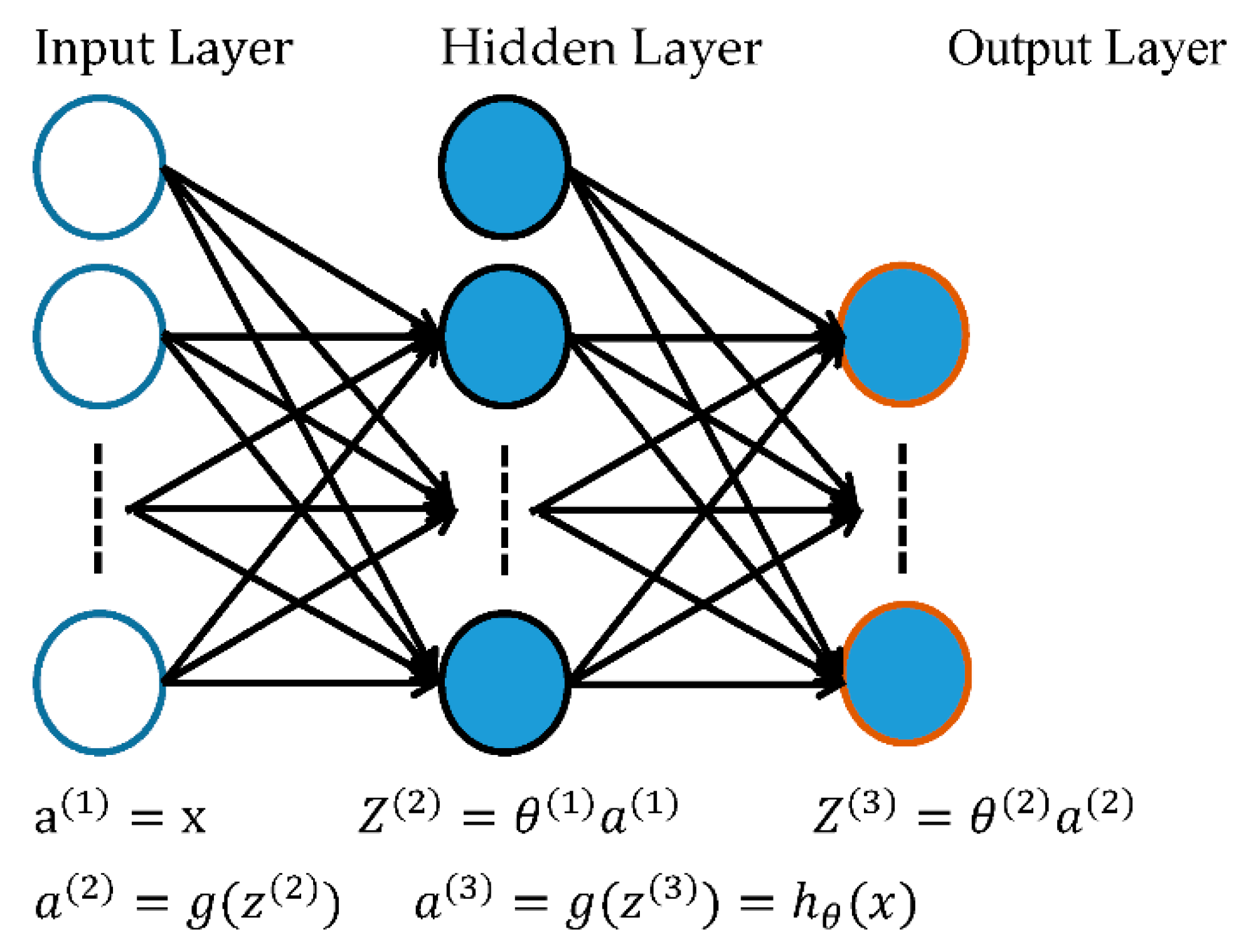
2. ANN Architecture

A neural network can be classified as either a static or dynamic network. The most common form of static network is the static feed-forward network. The output is calculated directly from the input through feed-forward connections, without feedback elements and delays such as backpropagation and cascade BPNN [13] (Figure 1). The result forms the argument of an activation function, φ, which acts as a filter and is responsible for the resulting neuron’s response as a single number [14].

$$Y_K\mathit{(}t\mathit{)}=\phi \left({\displaystyle \sum _{j=1}^n{w}_{\mathrm{kj}}\mathit{(}t\mathit{)}{x}_j\mathit{(}t\mathit{)}+}{b}_k\mathit{(}t\mathit{)}\right)$$

(1)

Here, x_j (t) is the input value of parameter j at time-step t; w_kj(t) is the weight assigned by neuron k to the input value of parameter j at time t; φ is a non-linear activation function; b_k (t) is the bias of the k-neuron at time t, and Y_K(t) is the output signal from neuron k at time t.

Dynamic networks, on the order hand, depend on both the current input to the network and the current or previous inputs, outputs, or states of the network. Examples of this are the recurrent dynamic network, with feedback connections enclosing several layers of the network, and the wavelet neural network, which is commonly used in time-series modeling [15,16,17].

Wavelet neural networks (WNNs), at their inception, attracted great interest because of their advantages over radial basis function networks as they are universal approximators but achieve faster convergence and are capable of dealing with the so-called “curse of dimensionality” [18,19,20,21]. The main characteristic of the wavelet NN is that wavelet functions are used in place of the sigmoid function as the non-linear transformation function in the hidden layer. Incorporating the time-frequency localization properties of wavelets, this technique has shown its advantages over the regular methods for complex non-linear system modeling.

There are two major kinds of WNN structure: the first has fixed wavelet bases, that is, the dilation and translation parameters of the wavelet basis are fixed while the output layer weights are adjustable; the second type is the variable wavelet bases, with adjustable dilation and translation parameters and output layer weights. In capturing the importance of the adjustable dilation parameter, which has an explicit physical concept, i.e., resolution, as it plays a significant role in wavelet analysis and approximation of a given function, the fuzzy wavelet network (FWNN) is adopted. This improves function approximation accuracy in terms of the dilation and translation parameters of wavelets while not increasing the number of wavelet bases. Compared with fuzzy neural networks, the FWNN is the second half of embedding wavelet neural networks into fuzzy neural networks. Here, the role of the fuzzy set is to determine the contribution of the sub-WNNs to the output of the FWNN [22]. As a result, the difficulties of selecting wavelets are reduced; additionally, wavelets with different dilation values under these fuzzy rules are fully utilized to capture various essential components of the system.

3. Methodology

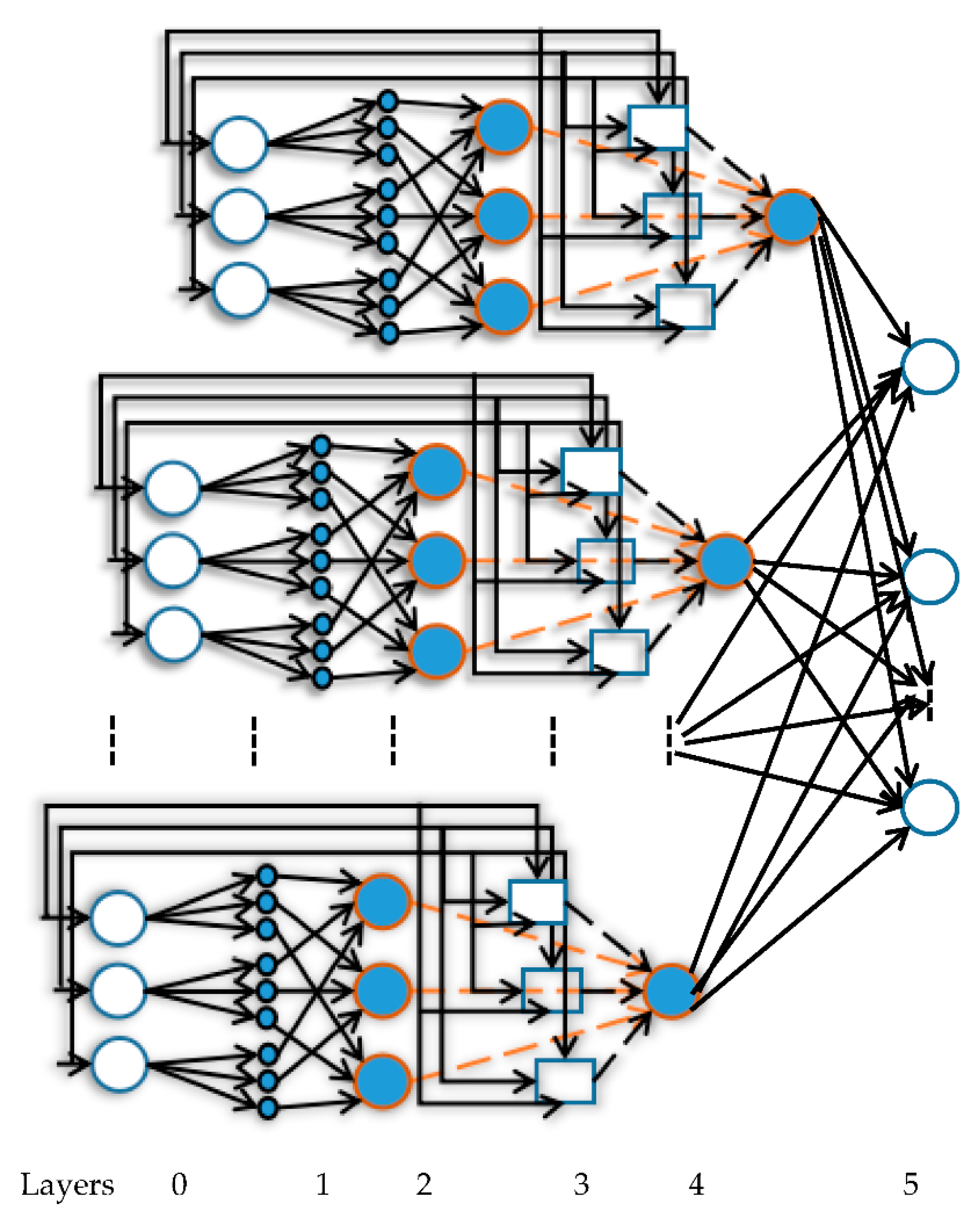
3.1. Structure of Fuzzy Wavelet Neural Networks

Considering that the BP network falls easily into local extreme value and that the wavelet neural network has poor adaptability to uncertain input information, the wavelet neural network embedded with a fuzzy neural network was used to evaluate the phase shift in the time-series signal. The FWNN harnesses the time-frequency localization properties of wavelets in evaluating the phase shift in specific frequency-defined signals.

The structure of the fuzzy wavelet neural network is shown in Figure 2. The network consists of four basic layers and a newly included fifth layer for EMT demodulation: the first layer is the input that is directly linked to the second layer, the membership function layer is also known as the fuzzification layer, the third layer is the inference layer, and the fourth layer is the defuzzification layer for the wavelet function, which conventionally produces the desired output. However, the desired output in EMT demodulation is a logical response with multiple output units. Therefore, an additional layer with a logical function, in this case, a sigmoid function, was introduced to produce a final output at the fifth layer.

3.2. Theory

Suppose there are Nr fuzzy, the IF-THEN rules are given as Rj:IF x1 is A1j AND x2 is A2j AND xi is Aij …… then,

$$y_j={\displaystyle \sum _{j=1}^{N_r}{w}_j\cdot {\mu }_j}$$

(2)

where x_i is the i-th input variable of the system (i = 1:N_in), A_ij is the fuzzy membership function, µA_ij (x_i) (j = 1:N_r) is a feature set of fuzzy languages, $w_j$ is the weight between the fuzzy layer and the output layer, µ_j is the output result of the fuzzy layer, and y_j is the output of the entire network.

Since the Gaussian membership function can maintain the original distribution of the data, the Gaussian function is selected as the membership function in the second layer. Therefore, A_ij, the fuzzy set, is characterized by the following Gaussian-type membership function, and µA_ij (x_i) is the grade of membership of x_i in A_ij, denoted as

$$\mu A_{ij}{=e}^{-}{\left({\left(\raisebox{1ex}{$\left(x_i-p_{ij}^1\right)$}\!\left/ \!\raisebox{-1ex}{$p_{ij}^2$}\right.\right)}^2\right)}^{\raisebox{1ex}{$p_{ij}^3$}\!\left/ \!\raisebox{-1ex}{$2$}\right.}$$

(3)

where $p_{{}_{ij}}^1$ represents the center of membership function, and $p_{{}_{ij}}^2$, and $p_{{}_{ij}}^3$ determines the width and shape of the Gaussian-type membership function, respectively. These are the free parameters of the membership functions, and these membership functions determine the contribution degree ${\mu }_j$ of each sub-wavelet network with a particular resolution.

For the third layer, each node in the layer represents a fuzzy rule R, and the output of each node can be expressed as:

$${\mu }_j\left(x\right)={\displaystyle \prod _i\mu A_{ij}\left(x_i\right)}$$

(4)

where ∏ represents the logical “and” operation, that is, the small operation.

Going into the fourth layer, wavelets are computed using the mother wavelet function. The selection of the mother wavelet depends on the application. Three mother wavelets are usually recommended: the Gaussian first-order partial derivative, the second derivative of the Gaussian (the so-called ‘‘Mexican Hat’’), and the Morlet wavelet. The activation function can be a wavenet (orthogonal wavelets) or a wave frame (continuous wavelets) [16]. Based on previous studies [16,23], two of the mother wavelets, the Mexican Hat and the Gaussian derivative, were initially selected, while the Mexican Hat function, which proved to be useful and to work satisfactorily in various applications, was finally adopted in this study. Therefore, the mother wavelet function is given as:

$$\phi \left(x\right)=\left({1-x}^2\right)e^{-0.5x^2}$$

(5)

As a mother wavelet function, this function has better fitting performance. According to the selected mother wavelet, the activation function in the neurons can be expressed as:

$${\phi }_j\left(z_{ij}\right)={\displaystyle \sum _{i=1}^{N_m}\left(1-z_{ij}{}^2\right)e^{-0.5z_{ij}{}^2}}$$

(6)

where

$$\forall z_{ij}=\left(\raisebox{1ex}{$\left(x_i-t_{ij}\right)$}\!\left/ \!\raisebox{-1ex}{$d_{ij}$}\right.\right)$$

(7)

Among them, t_ij and d_ij are the translation and dilation parameters of the wavelet, respectively, and the subscript ij indicates that the ith input corresponds to the jth wavelet neuron. The additional input of the fourth layer of the network is:

$$v_j={\displaystyle \sum _{k=1}^{N_j}{w}_j·{\phi }_{jk}}$$

(8)

while wj is the weight of the link between the hidden layer and output layer.

In the fourth layer, the input wavelet layer is multiplied by the node output of the third layer (fuzzy rule layer). The calculation formula is given as:

$$y\left(k\right)={\displaystyle \sum _{j=1}^{N_r}{\mu }_j\left(x\right)\cdot v_j}={\displaystyle \sum _{j=1}^{N_r}{y}_j}$$

(9)

Finally, the fifth layer combines the defuzzed output in proffering a logical prediction of the signal characteristic using a sigmoid function

$$Y\left(n\right)=g\left(w_{\mathit{nk}}\cdot y\left(k\right)\right)$$

(10)

where g represents the sigmoid function. Although the simple structure for logical response (prediction) involves adding a single layer to the conventional FWNN architecture, multiple layers can be included with additional features added to the fifth layer from the input layer during the training process to increase the effectiveness of the model in the demodulation process.

The parameters of the fuzzy wavelet neural network need to be automatically updated and adjusted during the network training process. The logical FWNN weights have two different effects on the network output. The first is the direct effect because a change in weight causes an immediate change in the output at the current time step (this first effect can be computed using standard backpropagation (BP)). The second is an indirect effect because some of the inputs to the layer are also functions of the weights. To account for this indirect effect, you must use dynamic BP to compute the gradients, which is more computationally intensive and expected to take more training time [24,25,26,27,28]. Here, the gradient descent method is used to adjust the network parameters with a major focus given to initialization. To update the parameters $p_{{}_{ij}}^r$, $t_{ij}$, $d_{ij}$, $w_j$ and $w_{nk}$, in order to obtain a good prediction effect, the optimal value of these parameters will be selected as the parameter value of the prediction part.

3.3. Defining the Input

In the input layer, the individual neurons are used for each input of an ANN. These inputs could be collected data or real-world inputs from physical sensors. However, in this study, pre-processing of the inputs is done to speed up the learning process and increase the accuracy of predictions of the network. Considering a binary phase modulation scheme, which is mostly chosen for electromagnetic telemetry (Figure 3), the phase-shift-characterizing section within a time series data is at or less than the quarter of a wavelength into and out of each signal being transmitted, meaning the optimal data requirement for an artificial intelligent demodulator system is only a fraction of the recorded signal, thereby reducing the training data and increasing the learning speed. However, digital demodulation requires bit-period synchronization; the receiver must be able to identify the boundaries between adjacent symbols. Therefore, extra sub-processing to obtain the correct start times for each representative wave of each symbol being transmitted is required. To address this problem, the cross-correlation technique is applied to determine the lag between a given transmitted correlation signal and the observed signal. Given a transmitted correlation signal S(t) and a received signal Sbl(t) in discrete form, the time lag is determined as:

TLag = T(idxS) − T(idxbl)

(11)

where idxbl and idxS are the time index of the maximum value of the cross-correlation of signal S(t) with Sbl(t) and itself, respectively, and Sbl(t) is a time fraction of the recorded signal obtained as:

$$S_{bl}\left(t\right)=\mathit{data}\left(1\mathit{to}\left(\raisebox{1ex}{$f_s$}\!\left/ \!\raisebox{-1ex}{$f_c$}\right.\right)\ast 2\right)$$

(12)

where f_s is the sample frequency, and f_c is the center frequency. For every time segment, the first data is recorded as time t0, which has an index of 1.

Finally, the time series is corrected as follows:

$$T_{\mathit{nw}}{=T}_{\mathit{lag}}\pm T_{data}$$

(13)

Additionally, the data can thus be separated into segments, starting from the corrected t0. The new signal is then formatted to match the neural network input. An example of the effect of time-shifted/sync data is shown in Figure 3.

The number of inputs of the network dictates how many sampled data are fed to the network at a time. In general, when the length of the sampled symbol (that is, a single wavelength) is equal to the number of inputs, the entire symbol is presented to the network at the same time, and the neural network will output a single decision for every slice of data presented to it. However, a combination of the reduced data from the initial data point (which is three wavelengths long) is used as an input in this study for data pre-processing. To avoid the complexity in the network learning process of simply demodulating the noisy raw data itself as well as analyzing it, the signal subtraction technique is also introduced. Here, a normalized combined signal, representative of the given phase transition symbols, is selected as the base signal S_sym(t) and then subtracted from normalized time-synchronized field recordings:

$$S_{att}\left(t\right)=S_{sym}\left(t\right)-S_{dat}\left(t\right)\pm \gamma$$

(14)

where $\gamma$ is a constant, with a value less than or equal to 0.05, used to ensure that the value of $S_{att}\left(t\right)$ does not equal zero.

As shown in Figure 4, this creates a new set of eight highly distinguishable and correlate-able combined two-phase transition signals (Figure 4). This process is introduced to further reduce the training time by introducing a variant of phase change in the network system to increase detectability, which is representative of binaries of ones and zeros for the full-wave regions and the almost-zero region, respectively. This reduces the training time and increases accuracy with noisy data.

Finally, the $S_{att}\left(t\right)$ and $S_{dat}\left(t\right)$ data are reduced by selecting the signal at the phase-characterizing section within a time series data, that is, less than a quarter of a wavelength into and out of each signal (Figure 4) and used as the input for the neural network with reduced network size and an increase in accuracy even with noisy data.

Demodulation of a BPSK signal can be considered a two-stage process: translation back to baseband, with the recovery of the bandlimited message waveform and the regeneration from the bandlimited waveform back to the binary message bitstream. Therefore, the neural network system will produce an output for each set of inputs presented to it. The choice of input size, as well as the number of connections, determines the balance between the spatial and temporal information that the neural network is attempting to learn. In this study, a completely spatial neural network will have the same number of inputs as samples per signal type and will only output one binary figure per input during training and simulation. Instead of the network, to output the reconstructed noiseless combined phase change system, logical output with binary values in the form of [1000000], [01000000], or [00000001] to represent either of the eight characterized combined phase shift signals is produced. This is rearranged in a logical response of ones and zeros: [10000000] = 0, [01000000] = 1, [00100000] = 0, [00010000] = 1, [00001000] = 0, [00000100] = 1, [00000010] = 0, [00000001] = 1, accordingly, to reproduce the coded transmitted signal. This type of detection is similar to number detection using multiple frames of low-resolution data [29], with the final output being the detected number.

3.4. Initializing of Parameters

For the training algorithm’s initialization, wavelets and membership functions parameters are set from a uniform distribution. From Equations (3) and (7)–(10), we can see that the parameters to be trained in the FWN will be $p_{{}_{ij}}^r$, $t_{ij}$, $d_{ij}$, $w_j$, and $w_{nk}$. The initial parameters $p_{ij}^1,$ and $p_{ij}^2$ are chosen to be the weighted mean and standard derivation of the input data, respectively, while $p_{ij}^3$ is selected as a random number in a pre-selected range (this is discussed in the next sub-section) to shape the Gaussian-type membership function. In this framework, the initialization of the wavelet parameters is based on the input domains defined by the examples of the training sample [30,31]. The following expressions were used in the initialization of the translation $t_{ij}$ and dilation $d_{ij}$ parameters,

$$t_{ij}=\mathit{0}\mathit{.}\mathit{5} \ast \left(X_{\mathit{min} i}{+X}_{\mathit{max} i}\right)$$

(15)

$$d_{ij}=\mathit{0}\mathit{.}\mathit{2} \ast \left(X_{\mathit{max} i}{-X}_{\mathit{min} i}\right)$$

(16)

where $X_{\mathit{max} i}$ and $X_{\mathit{min} i}$ are defined as the maximum and minimum of input $X_i$. Lastly, $w_j$ and $w_{nk}$ can be selected randomly, as obtained in this study.

3.5. Training a Fuzzy Wavelet Network with Backpropagation

After the initialization phase, the network is further trained in order to find the weights that minimize the cost function. In our implementation, backpropagation (BP) was used to adjust the free parameters of the FWNN models. This technique has been used by several authors, and it is the most frequently used technique to train FWNNs [30,32,33,34,35,36]. The BP is less fast but also less prone to sensitivity to initial conditions than higher-order alternatives. However, the use of wavelet functions in neural network structures reduces the inconvenience that it may get stuck on a local minimum of the error surface and that the training convergence rate is generally slow [32,37]. Typically, mean squared error (MSE) is used as the cost function with the BP algorithm [14]. Other technique includes the use of the maximum correntropy criterion (MCC) and the extended Kalman filter (EKF) algorithm [15,32].

Explicit formulas for the partial derivatives of the output of the FWNN with respect to each component of the parameter vector are listed as follows:

$$\frac{\partial \xi }{\partial w_{nk}}=\frac{\left(Y_{}\mathit{(}n\mathit{)}-Y_{}^d\mathit{(}n\mathit{)}\right)}{{\displaystyle \sum _{k=1}^c{y}_k}}·y_k$$

(17)

$$\frac{\partial \xi }{\partial w_j}=\left(Y_{}\mathit{(}t\mathit{)}-Y_{}^d\mathit{(}t\mathit{)}\right)•w_{nk}•{\mu }_j\mathit{(}x\mathit{)}•{\phi }_j(z)/{\displaystyle \sum _{j=1}^{N_r}{\mu }_j\mathit{(}x\mathit{)}}$$

(18)

$$\begin{array}{l}\frac{\partial \xi }{\partial d_{ij}}=\left(Y_{}\mathit{(}t\mathit{)}-Y_{}^d\mathit{(}t\mathit{)}\right)•w_{nk}•{\mu }_j\mathit{(}x\mathit{)}•w_j/{\displaystyle \sum _{k=1}^{N_j}{\mu }_k}\\ •\raisebox{1ex}{$\mathit{(}3.5z_{ij}^2-z_{ij}^4-0.5\mathit{)}{e}^{-\raisebox{1ex}{$z_{ij}^2$}\!\left/ \!\raisebox{-1ex}{$2$}\right.}$}\!\left/ \!\raisebox{-1ex}{$\mathit{(}\sqrt{a_{ij}^3}\mathit{)}$}\right.\end{array}$$

(19)

$$\begin{array}{l}\frac{\partial \xi }{\partial t_{ij}}=\left(Y_{}\mathit{(}t\mathit{)}-Y_{}^d\mathit{(}t\mathit{)}\right)•w_{nk}•{\mu }_j\mathit{(}x\mathit{)}•w_j/{\displaystyle \sum _{k=1}^{N_j}{\mu }_k}\\ •\raisebox{1ex}{$\mathit{(}3z_{ij}^{}-z_{ij}^3\mathit{)}{e}^{-\raisebox{1ex}{$z_{ij}^2$}\!\left/ \!\raisebox{-1ex}{$2$}\right.}$}\!\left/ \!\raisebox{-1ex}{$\mathit{(}\sqrt{a_{ij}^3}\mathit{)}$}\right.\end{array}$$

(20)

$$\begin{array}{l}\frac{\partial \xi }{\partial p_{ij}^1}=\left(Y_{}\mathit{(}t\mathit{)}-Y_{}^d\mathit{(}t\mathit{)}\right)•w_{nk}•\left(v_j-y\mathit{(}k\mathit{)}\right)/{\displaystyle \sum _{j=1}^{N_r}{\mu }_j\mathit{(}x\mathit{)}}\\ •{\mu }_j\mathit{(}{x}_i\mathit{)}{p}_{ij}^3\frac{{\left|\raisebox{1ex}{$x_j-p_{ij}^1$}\!\left/ \!\raisebox{-1ex}{$p_{ij}^2$}\right.\right|}^{p_{ij}^3}}{\left(x_j-p_{ij}^1\right)}\end{array}$$

(21)

$$\begin{array}{l}\frac{\partial \xi }{\partial p_{ij}^2}=\left(Y_{}\mathit{(}t\mathit{)}-Y_{}^d\mathit{(}t\mathit{)}\right)•w_{nk}•\left(v_j-y\mathit{(}k\mathit{)}\right)/{\displaystyle \sum _{j=1}^{N_r}{\mu }_j\mathit{(}x\mathit{)}}\\ •{\mu }_j\mathit{(}{x}_i\mathit{)}\frac{p_{ij}^3}{p_{ij}^2}{\left|\frac{x_j-p_{ij}^1}{p_{ij}^2}\right|}^{p_{ij}^3}\end{array}$$

(22)

$$\begin{array}{l}\frac{\partial \xi }{\partial p_{ij}^3}=\left(Y_{}\mathit{(}t\mathit{)}-Y_{}^d\mathit{(}t\mathit{)}\right)•w_{nk}•\left(v_j-y\mathit{(}k\mathit{)}\right)/{\displaystyle \sum _{j=1}^{N_r}{\mu }_j\mathit{(}x\mathit{)}}\\ •-\frac{{\mu }_j\mathit{(}{x}_i\mathit{)}}{2}{\left|\frac{x_j-p_{ij}^1}{p_{ij}^2}\right|}^{p_{ij}^3}\mathit{ln}{\left(\frac{x_j-p_{ij}^1}{p_{ij}^2}\right)}^2\end{array}$$

(23)

where $i=\mathit{1}\mathit{,}\mathit{2}\mathit{,}\dots \dots \mathit{,}c$ is the index of fuzzy rules, $j=\mathit{1}\mathit{,}\mathit{2}\mathit{,}\dots \dots \mathit{,}\mathit{q}$ the index of input variables, and $k=\mathit{1}\mathit{,}\mathit{2}\mathit{,}\dots \dots \mathit{,}\mathit{S}$ the index of wavelets. The logistic layer can be extended into several layers to increase accuracy in the logistic prediction phase, and the gradient descent will follow the general computation of the partial derivative at each added layer, which will involve the calculation of the sigmoid function’s gradient.

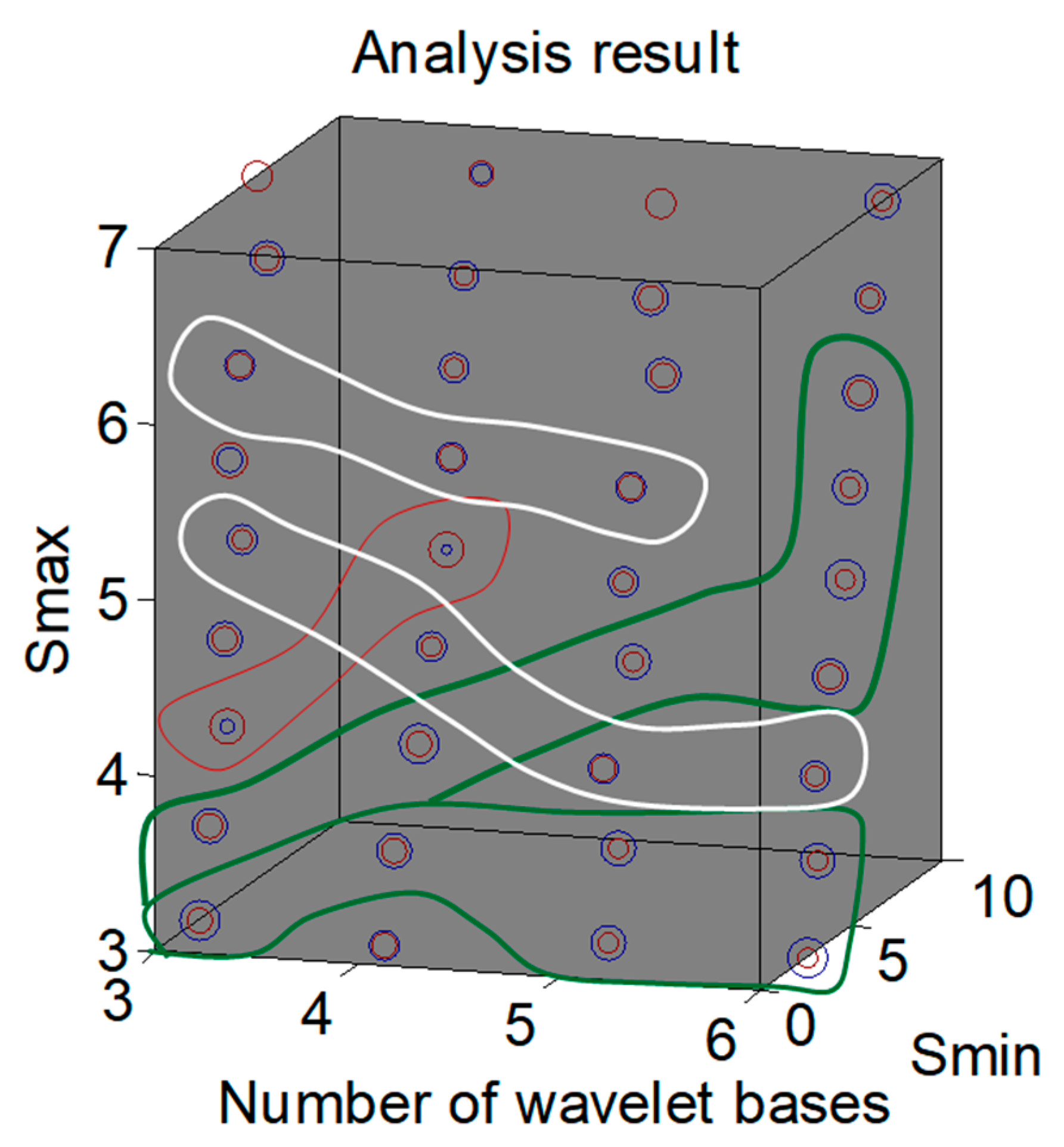
3.6. Estimating the Number of Wavelet Bases and the Pre-Selected Range for $p_{ij}^3$

In general, fuzzy WNN methods combine wavelet theory with fuzzy logic and neural networks. The fuzzy models consist of a set of rules, and each rule acts like a “local model” by using a fuzzy set to partition the input space into local fuzzy regions. Each fuzzy rule corresponds to a sub-WNN consisting of wavelets with a specified dilation value (i.e., resolution). Thus, the sub-WNNs at different resolution levels are used to capture different behaviors (global or local) of the approximated function. Here, the role of the fuzzy set is to determine the contribution of the sub-WNNs to the output of the FWN. As a result, the difficulties of selecting wavelets are reduced; additionally, wavelets with different dilation values under these fuzzy rules are fully utilized to capture various essential components of the system. In general, learning is fully automatic and does not require any external intervention, making these methods very useful in practical applications, for instance, during the gaming and field testing of sensors.

Among the scaling function associated to these wavelets, the $p_{ij}^3$ controls the shape of the membership function and, thus, determines the contribution of the sub-WNNs, with multiple resolutions to the output of the FWNN. Therefore, in a multi-frequency data/signal, frequency-focused output can be obtained within a regulated range of $p_{ij}^3$. In other words, the value of $p_{ij}^3$ affects the selective shape of the output signal and, in turn, the output resolution.

Though functional approximators, other than wavelets, may have a universal approximation property, in general, they respond to the multi-resolution property of the sub-WNNs/wavelets. That is, the wavelets with coarse resolution can capture the global (low frequency) behavior easily, while the wavelets with fine resolution can capture the local behavior (higher frequency) of the function accurately. In general, the model is refined as more data are furnished to the system. With only a few data points, the information on the underlying surface is small, and a low-resolution description of the system is appropriate, while with an increasing number of data points, a higher resolution may be justified. Therefore, the number of wavelet bases (“N”) used determines the level of variation and disparity in the wavelet function, and, in turn, increases either the smoothness or roughness or wavelength of the predicted output. Therefore, the change in the characteristic of the output signal with respect to the variation in the values of the number of wavelet bases and the pre-selected range for $p_{ij}^3$ and the possible trade-off between the two properties is worth considering.

In this section, we trained the FWNN using a range of values for the number of wavelet bases, n_range = 3:7, and $p_{ij}^3$ as S_max = 3:7 and S_min = 1.5:5.5, using the same data as [38]. S_max and S_min represent the maximum and minimum values for $p_{ij}^3$, respectively, within a single range. The number of features in the data is 5, meaning the common number of wavelet bases to be used will be 5. Furthermore, two properties obtained from the output signal (data)—(1) slope around the peaks across the data, which is a measure of the curvature, and (2) standard deviation of error (SDE) across the signal—were used to assess the possible trend in the output signal. Figure 5 shows the cross-plot of the above properties. The blue circle represents the slope around the peak across the data, while the red circle represents the SDE. The higher the value of the properties, the larger the radius of the circle.

The following trends were observed in the cross-plot:

Trend 1: Low SDE—High slope. This is a common response, with a low range of values for $p_{ij}^3$, and the value along the plot of N equals 6, which is traced with a green marker. A plot of the corresponding output signal representing this trend is shown in Figure 6. The predicted output (red) shows a very close similarity with the expected result (blue), meaning high accuracy output, high/fine resolution data prediction, and a wider range of composite frequency.

Trend 2: High SDE—Low slope. This shows a non-continuous linear trend between the number of wavelet bases “N” and the pre-selected range for $p_{ij}^3$ “S_range” (highlighted red), limited to values below 5. A plot of the corresponding output signal representing this trend is shown in Figure 6. The predicted output signal (red) represents a low pass filter response with a very high wavelength.

Trend 3: Low SDE—Relatively low slope. This shows mostly an inverse relationship between the number of wavelet bases “N” and the pre-selected range for $p_{ij}^3$ “S_range”, which is traced with a white marker; that is, as N increases, the expected value for S_range reduces. A plot of the corresponding output signal representing this trend is shown in Figure 6. The predicted output (red) shows similarity with the expected result (blue) but with better curvature and low pass filtering characteristics.

In total, the signal with the lowest slope and SDE is represented at N equals 4 and an S_range of 7. A plot of the corresponding output signal with these parameters is shown in Figure 6. The predicted output signal is representative of a strong low pass filter with a high curvature. Therefore, considering the obtained trends and their respective predicted output signal, a more appropriate number of wavelet bases “N” and the range for $p_{ij}^3$ “S_range” could be selected to fit the desired output, especially when dealing with noisy signals or frequency-based output prediction. That is, quick analysis can be performed on a few pieces of data to select the best “N” and “S_range” that produces the desired output, as applied in the next section, where noisy data are considered in EMT demodulation.

4. Examples

In this section, we demonstrate the performance of the FWNN on synthetic EMT data set with three noise variations and a pseudo-synthetic field data set using the complete data processing workflow with adaptive processing [12]. The FWNN system is applied for constructing a prediction model of the signal code using the Matlab script run on a GTX 950M GPU computer with 8 gig RAM to train and execute the demodulation appropriately.

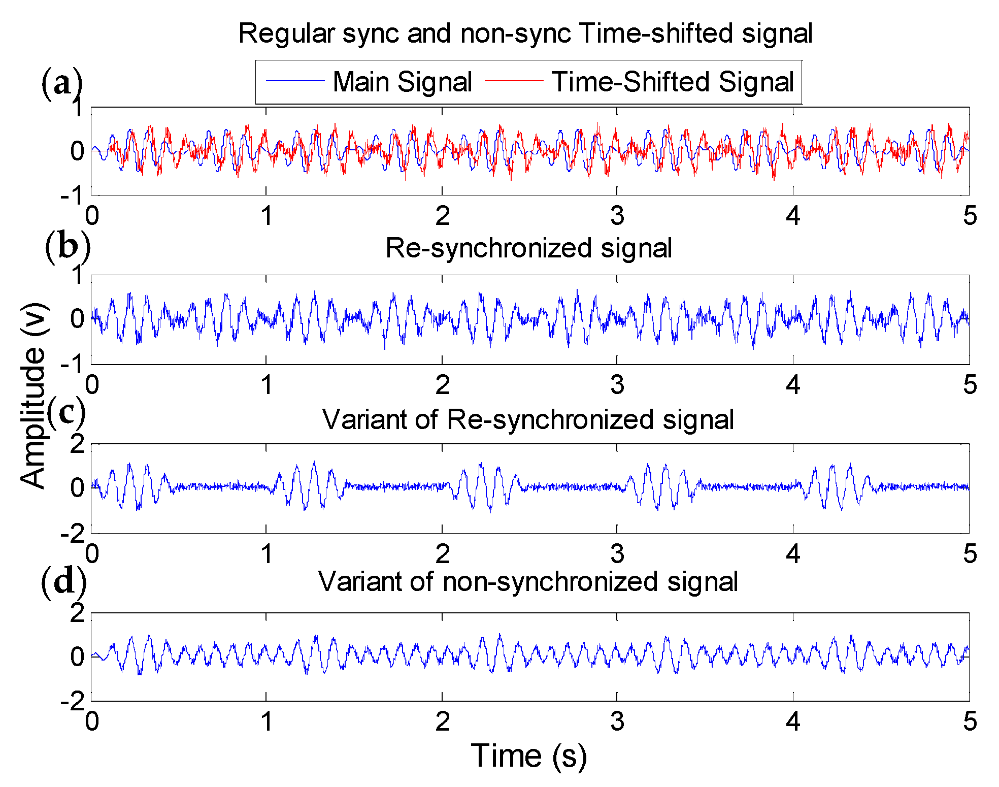
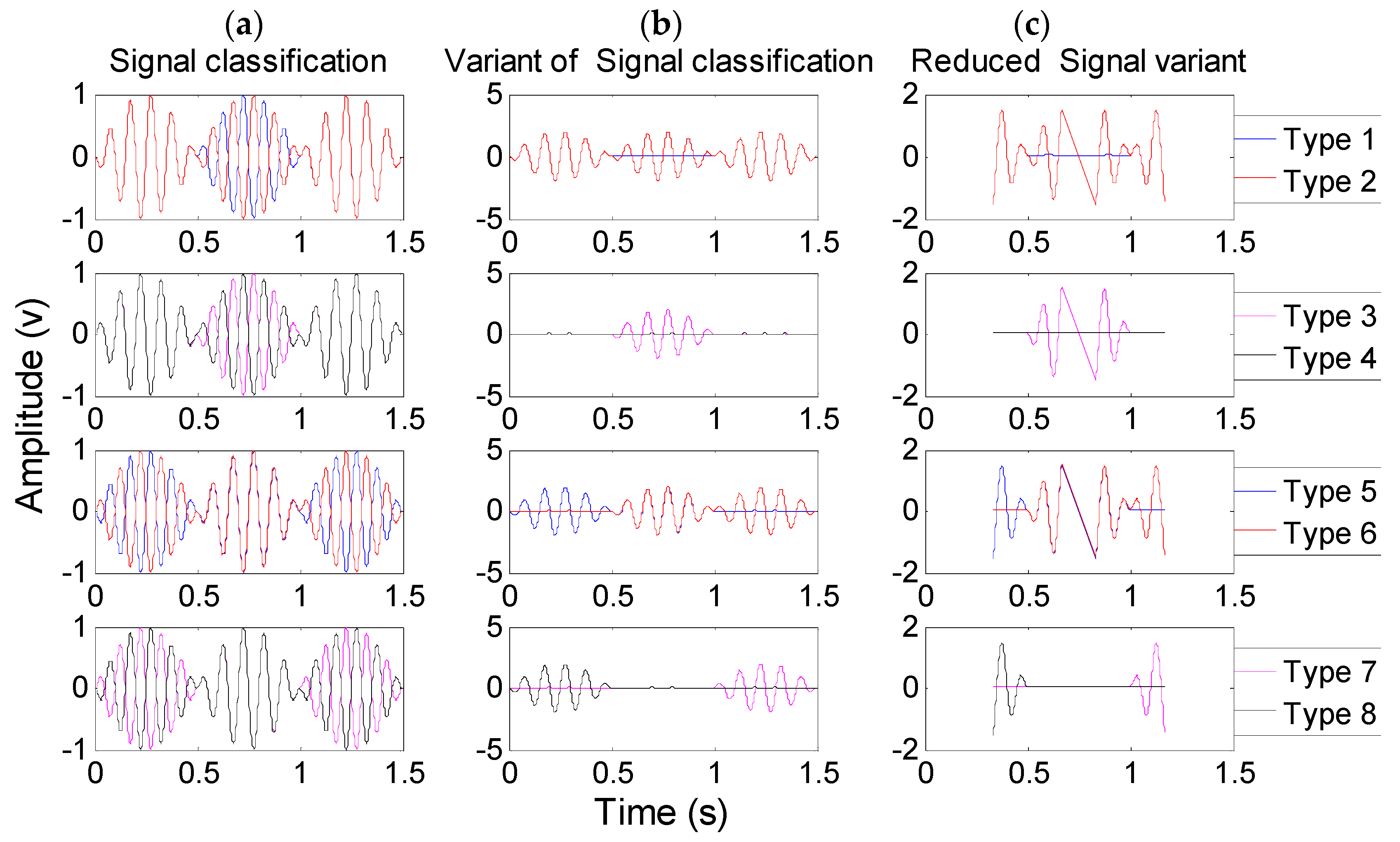
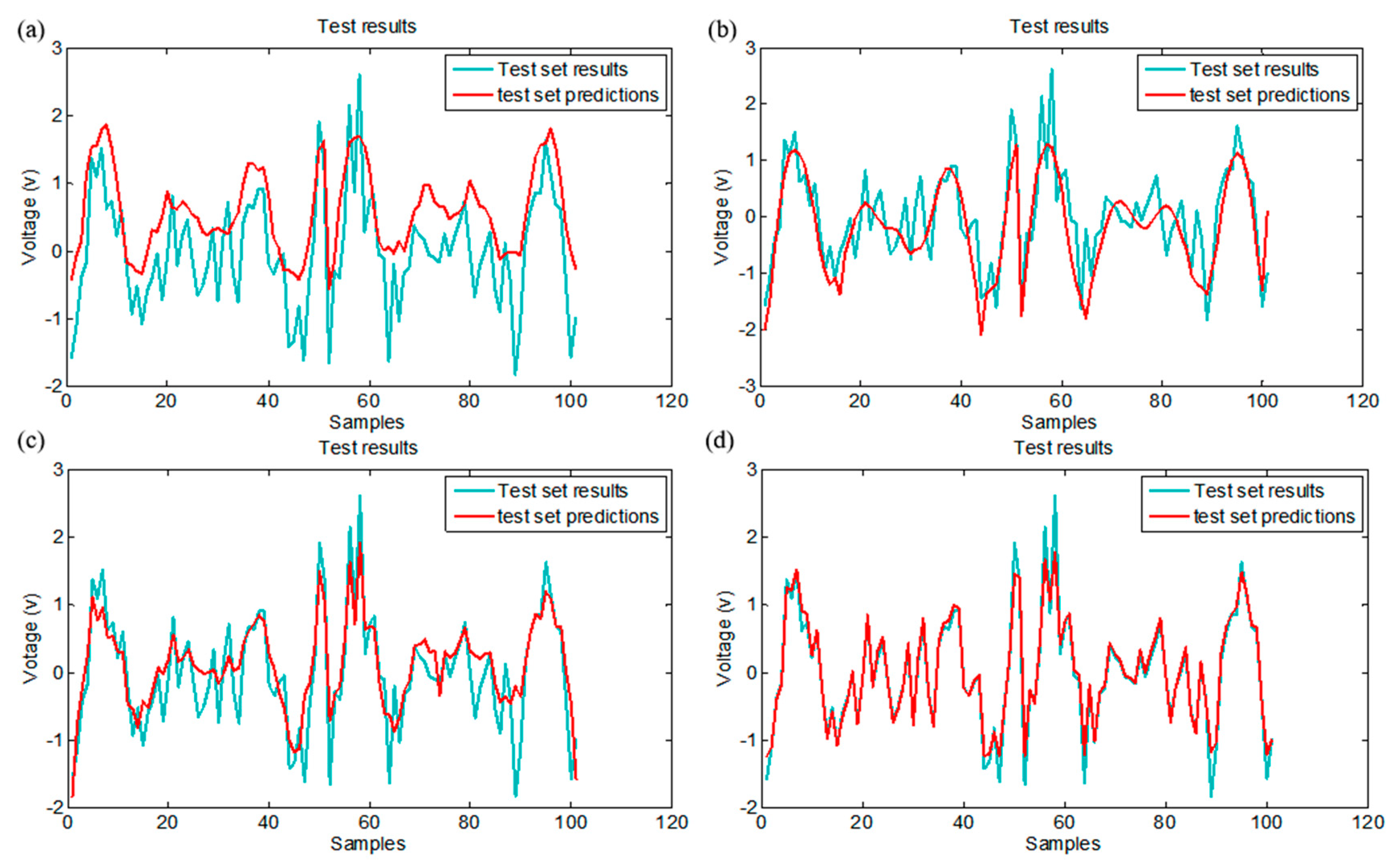
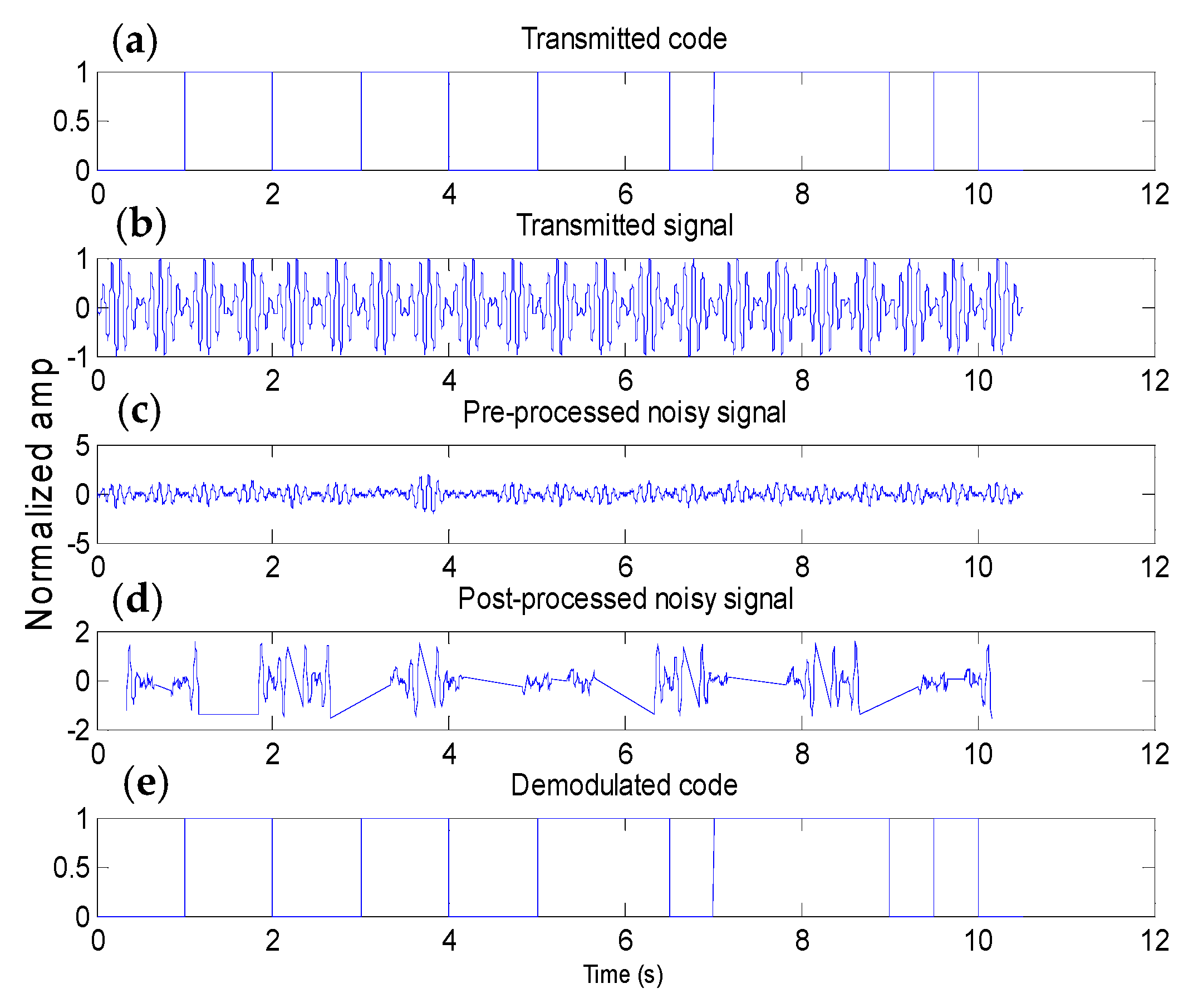
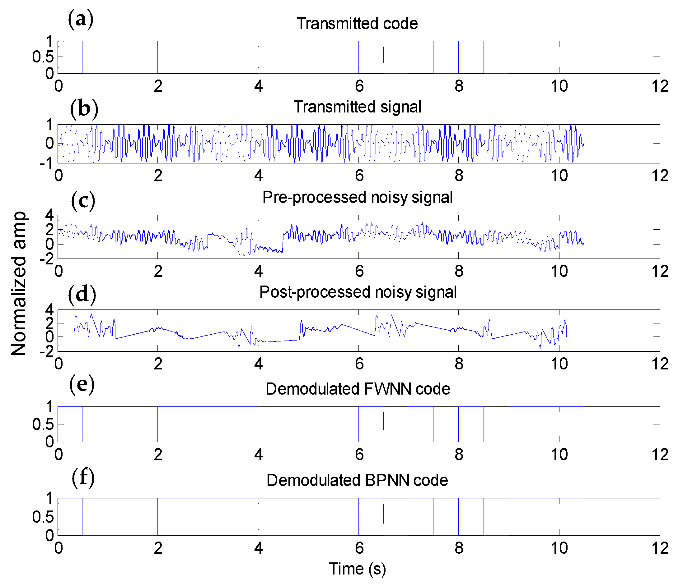
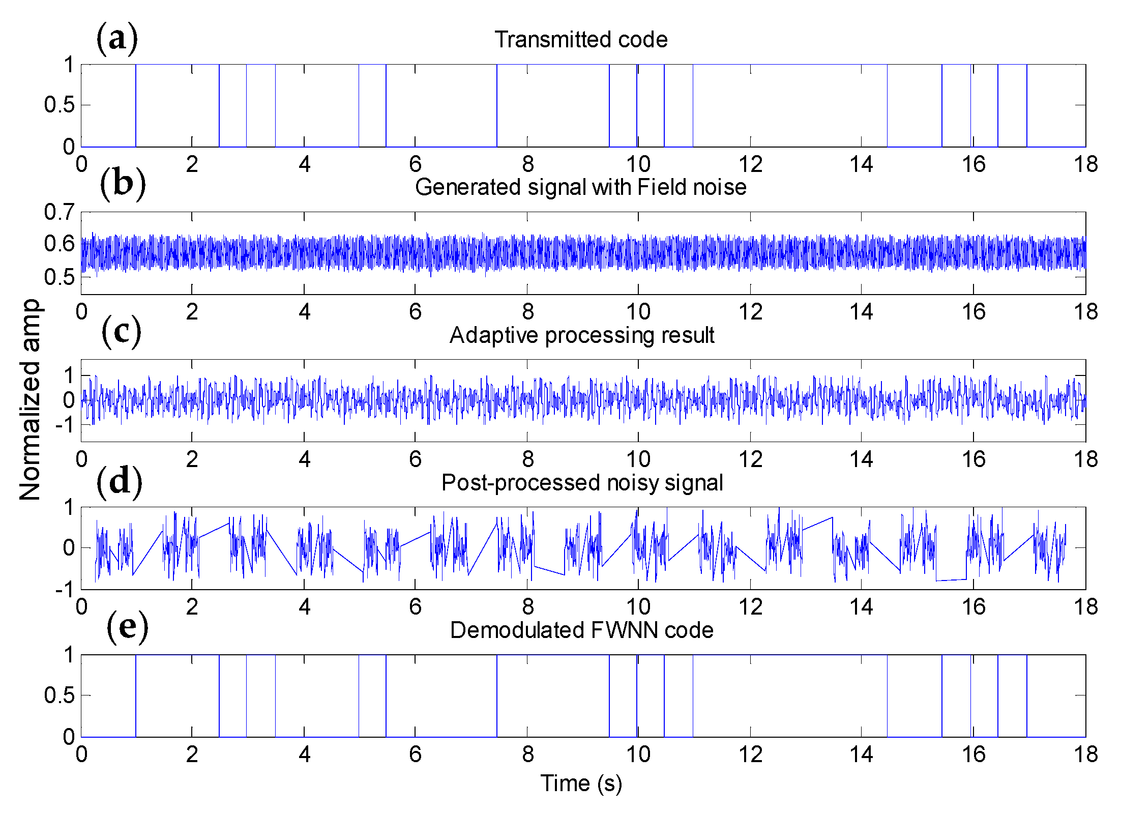
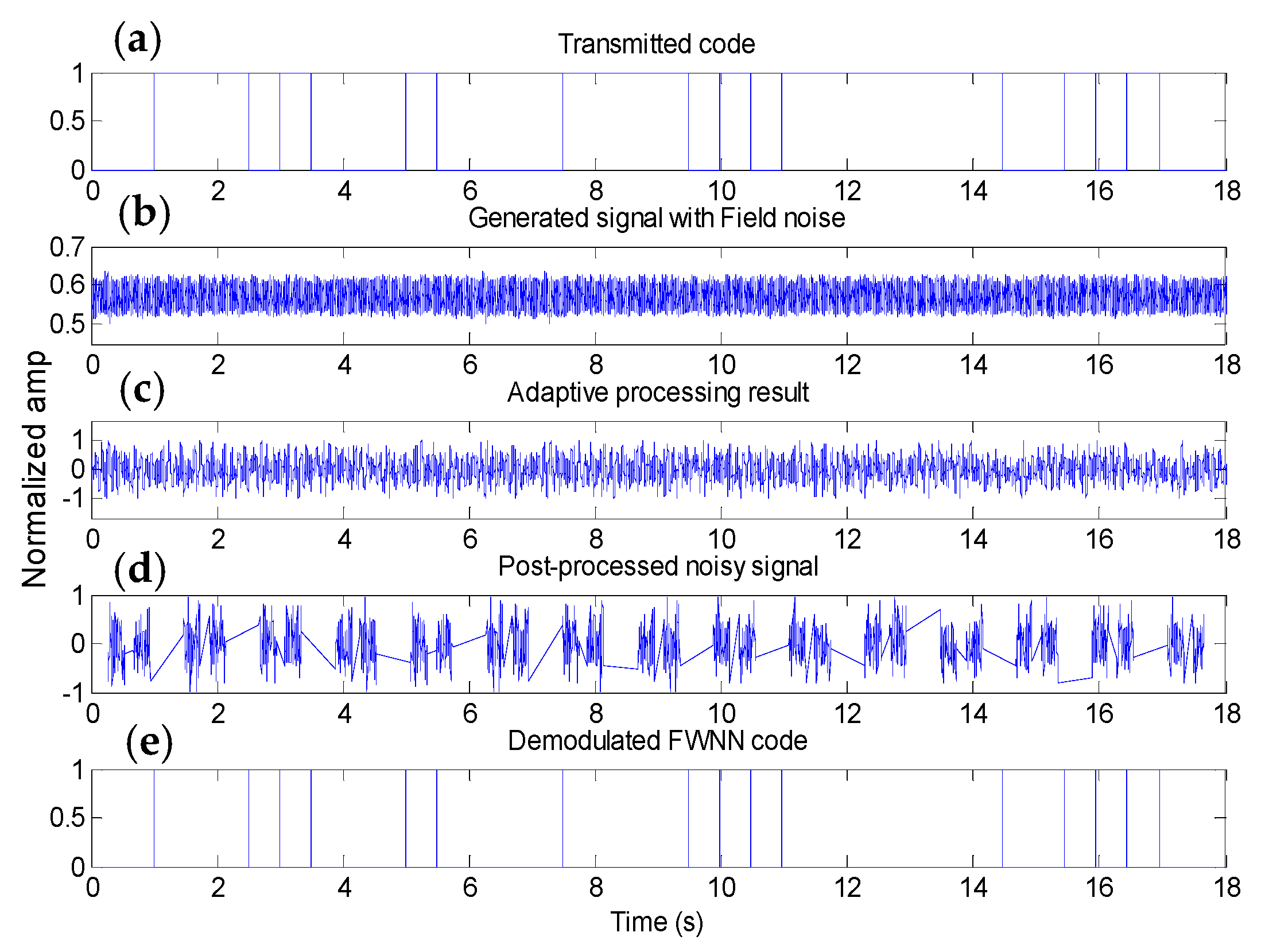
4.1. Comparison of the FWNN with BP Using Synthetic Data with Three Noise Variants

In this section, synthetic data with defined noise characteristics added to the modulated signal are demodulated to check the robustness of the FWNN and its filtering capability. The test system is composed of data resampling and demodeling. Data reduction is the first part of the system that leads to the derivation of the more distinguishable attributes of the transmitted signal.

Similarly, prior to the training of the FWNN system, the number of wavelet bases “N” and the pre-selected range for $p_{ij}^3$ to be used were selected within a range of [5:20] and [1.5:5.5; 3:7], respectively. This was done using 352 data sets with multiple noise characteristics such as white noise, red noise, and blue noise. Figure 7 shows the representative of the pre-selected values with their respective test results. The results are presented in sections, with 101 samples per section. The test set result in green represents the noisy EMT data, while the test set prediction in red is the FWNN output signal. In the general application of the FWNN, Figure 7d, with the matching test set prediction, would be the required result, meaning N equals 8 and $p_{ij}^3$ ranges from 5.5 to 7 would be our selected values. However, in EMT demodulation, Figure 7a,b has the best representation of the required denoised signal, similar to Figure 4 Type 2. Therefore, in this study, a value of 8 was selected for the number of wavelet bases (”N”) and an adopted range of [4 6.5] was pre-selected for $p_{ij}^3$. The value of $p_{ij}^3$ is allowed to change freely within the given range during the iteration process.

Using the selected values, we trained the FWNN with a logistic response using 680randomly selected datasets with varying noise types. The training time was approximately 8 h. Thereafter, we evaluated our method on a randomly selected test set with 54 datasets. The recorded cost was 0.02, and the prediction result accuracy varied between 92.5% to 100% accuracy, with the SNR ratio varying from −20 to 10 dB. Figure 8 and Figure 9 show part of the results for the retrieved code. The recovered code in Figure 8 was a 100% match with the transmitted code, as against that of Figure 9, where the latter codes were a mismatch due to the low signal-to-noise ratio.

We further illustrate the performance of the proposed algorithms by comparing the output of the demodulated code with the result from the conventional BP technique in a system with an identical scenario and noise characteristics, as given in

Table 1. Comparison of our FWNN with BP. The same number of unknown parameters (NUPs) was used for the training for each noise characteristic and SNR.

Method		Time (s)			% Accuracy
	Noise Characteristic	SNR-15	SNR 1	SNR-10	SNR-15	SNR-1	SNR-10
FWNN	AWGN	0.45	0.38	0.34	93.1	100	100
	Red and blue	0.42	0.42	0.44	100	100	100
	Pink and violet	0.40	0.39	0.32	100	98	100
BP	AWGN	0.12	0.19	0.15	87.5	95	100
	Red and blue	0.21	0.21	0.23	98.8	97.5	100
	Pink and violet	0.15	0.15	0.14	97.5	100	100

. The test for each noise variation is presented by a comparative figure and the information in the general table.

The first is Figure 10, which depicts the BP and FWNN results when the transmitted signal noise is the combination of red and blue noise, with an SNR of 10 dB. The recovered codes were a good representation of the transmitted code. That is, high accuracy is attainable by both methods when the SNR is equal to or higher than 10 dB. Similarly, both methods recorded high accuracy with the pink and violet noise even at an SNR of 1 dB (Figure 11).

However, for other noise characteristics, the accuracy of the BP technique was reduced to 97.5% and 95%, respectively, for the pink and blue noise and the AWGN noise, respectively (Table 1). Last is the performance of both techniques in the presence of AWGN noise. The results show a less accurate result for both methods with an SNR value of −15 dB (Figure 12) and the BP method having an accuracy of 87.5% and the FWNN an accuracy of 93.1% (Table 1). The displayed figures show the representative section of the obtained responses from the different techniques.

The effectiveness of the two techniques is established, as observed from the percentage accuracy in Table 1, which details the networks’ performance under different signal-to-noise ratios. The two networks performed excellently, with a moderately low SNR value of 1. However, as the SNR decreases, the performance index decreases, as expected, while the % accuracy remained mostly constant for the FWNN system as against a reduction in the value obtained for the BP network. The average time for the FWNN operation was recorded to be 0.40 s; although this is generally twice the time required for the BP operation, it is still fast enough for real-time operation. This operation time can, however, be slower if the value of N is increased drastically.

In general, it is found that the FWNN yielded the best PSNR values and achieved performance improvements in all kinds of noise levels. Furthermore, the comparison of the average processing time of the image recorded in Table 1 indicates that the methods have quite a small computational cost.

4.2. Comparison of the FWNN with BP Using Pseudo-Synthetic Data

In general, artificial learning methods rely heavily on large amounts of training data that significantly creates the wide characteristic filter required for accurate prediction over a wide range of scenarios. Therefore, to work out the effectiveness of the FWNN method with real data, we adopted the complete data processing workflow with adaptive processing in removing ELF-EM band noise and demodulating generated pseudo-synthetic EMT data. Pseudo-synthetic EMT data was adopted to fill the void of cogent field data. The pseudo-synthetic EMT data were generated by means of combining binary phase shift key code modulation and actual field noise. Figure 13 shows a typical schematic diagram of the EMT/EM MWD signal processing workflow with signal code recovery.

Electromagnetic telemetry data were acquired during a drilling operation in Sichuan province, China. The starting depth of the downhole transceiver was about 2000 m. A phase-shift-coded signal with a center frequency of 10 Hz and a shift frequency of 2 Hz was transmitted from the insulating gap along the drill string, which was outside the borehole casing. The electrode array used in EM telemetry signal measurement is described in [12]. The voltage difference between dipoles (L1 to L10) was recorded using the DRU 45 system developed by the Institute of Geology and Geophysics, Chinese Academy of Sciences, at a sampling frequency of 2400 Hz. In this study, we considered the performance of the technique by considering only the field noise characteristics and convolving it with the generated binary phase shift signal. The amount of generated data set was 465, and all of them were of sizes 1275 × 1. Moreover, these data were randomly divided into three sets. Specifically, 350 of these data were used as the training set, 65 as the validation set, and the remaining 50 were used for testing. Large parts of the initially generated data were included in the training set, increasing the total training data set to 720.

Considering a sinusoidal carrier, if it is modulated by a bi-polar bitstream, its polarity will be reversed every time the bitstream changes polarity. This, for a sinewave, is equivalent to a phase reversal (shift), and the output is similar to the adopted BPSK signal. A binary phase shift signal was generated using a sample rate of 2400 Hz, signal frequencies of 10 Hz, and a period of 0.5 s. In assessing the effectiveness of the FWNN technique, the BPSK signal amplitude was varied between 0.05 and 0.0002 V to allow for an assessment of the technique under different signal-to-noise ratios (SNRs).

Figure 14, Figure 15 and Figure 16 show the variation in the adaptive processing result, with changes in the signal-to-noise ratio from 8.3 × 10⁻² to 8.3 × 10⁻⁴ and the FWNN-recovered code. As observed in Figure 14, the adaptive processing result was excellent and easy to decode using the FWNN technique. However, as the SNR reduces, the effectiveness of the adaptive processing reduces, considering the same processing time for all the signals. However, the accuracy of the FWNN techniques remained constant, thereby retrieving the transmitted code effectively.

The obtained results reiterate the effectiveness of the proposed workflow. Likewise, the above techniques do not require the spectral characteristics of EMT/EM MWD data in the real-time denoising and demodulation of the acquired data. Additionally, the inclusion of the FWNN in the coded signal recovery process reduces the pressure on adaptive processing in producing totally smoothly varying processed data. The above point, therefore, reduces the working time for coded signal recovery by eliminating the determination of spectral characteristics in the field and reducing the working time of adaptive processing.

Additionally, synthetic data analysis and pseudo-field data processing show that the algorithm can solve practical engineering problems and provide a reference to field technicians.

5. Conclusions

This paper presents the development of a fuzzy wavelet neural network model with a logistic response for EMT/EM MWD and validates its prediction on the pseudo-synthetic EMT data that was generated by means of combining binary phase shift key code modulation and actual field noise. In the implemented scheme, the frequency-time characteristics of the predicted signal are controlled by selecting an appropriate number of wavelet bases (“N”) and the pre-selected range for $p_{ij}^3$ to be used, prior to the training of the FWNN system. In addition, the problem of digital communication synchronization in the EM MWD environment using neural networks was addressed by adopting the cross-correlation technique. In order to reduce the computational cost and increase prediction accuracy, post-processing steps to reduce the data volume and obtain a more characterized attribute of the phase shift signal were introduced.

The FWNN result was compared with that of the commonly used BPNN. Although both techniques performed well, with moderately low SNRs, sharing common response characteristics with expectation–maximization, the FWNN provided an advantage in terms of performance, with EMT/EM MWD signals with very low SNRs. It should be noted that the proposed structures differ from the usual time-series prediction models since they include a logistic layer for transmitted code prediction.

The full EMT/EM MWD processing workflow results, including both adaptive processing and signal demodulation, show that the proposed FWNN prediction model provides an accurate return of the transmitted code for the pseudo-synthetic datasets. Further work could explore more methods of obtaining the start and stop times as well as the deduction of performance when the transmitter and receiver are out of synchronization. In future work, the present approach will be enhanced by adding a recurrent step in the algorithm’s weather information, such as temperature. Additionally, the application of the above technique in various real field data will be pursued as the opportunity presents itself.

References

- IEEE. Fifty Years of Signal Processing: The IEEE Signal Processing Society and its Technologies, 1948–1998. Available online: https://signalprocessingsociety.org/our-story/society-history (accessed on 1 November 2020).
- Suh, A.E. Noise Cancellation in Electromagnetic Measurement While Drilling Using Spectral Subtraction. Master’s Thesis, California Polytechnic State University, San Luis Obispo, CA, USA, 2004. [Google Scholar]
- Lu, C.D.; Du, H.B.; Wang, J.H.; Zhang, C.A. Design of EM-MWD Signal Receiver Circuit Based on STM32. Chin. J. Eng. Geophys. 2015, 12, 423–427. [Google Scholar]
- Long, L.; Chen, Q.; Liu, F. Research on eliminating interference signal algorithm of EM-MWD. Chin. J. Sci. Instrum. 2014, 35, 2144–2152. [Google Scholar]
- Whitacre, T.P. A Neural Network Receiver for EM-MWD Communication. Master’s Thesis, California Polytechnic State University, San Luis Obispo, CA, USA, 2011. [Google Scholar]
- Li, F.K.; Yang, Z.Q.; Fan, Y.H.; Hao, C.; Zhu, G.; Jin, Y.; Fang, J.; Li, T. Multiple Combinational Algorithm to Adaptively Track and Detect Measurement While Drilling Electromagnetic Wave Signal. In Proceedings of the 12th International Symposium on Antennas, Propagation and EM Theory (ISAPE), Hangzhou, China, 3–6 December 2018; pp. 1–5. Available online: https://ieeexplore.ieee.xilesou.top/abstract/document/8634120 (accessed on 13 January 2020).
- Abiodun, O.I.; Jantan, A.; Omolara, A.E.; Dada, K.V.; Mohamed, N.A.; Arshad, H. State-of-the-art in artificial neural network applications: A survey. Heliyon 2018, 4, e00938. [Google Scholar] [CrossRef] [PubMed] [Green Version]
- Li, H.; Zhang, Z.; Liu, Z. Application of Artificial Neural Networks for Catalysis: A Review. Catalysts 2017, 7, 306. [Google Scholar] [CrossRef]
- Farhad, E. Extremely Low Frequency (Elf) Signal Processing for Electric Borehole Telemetry. Ph.D. Thesis, Oklahoma State University, Stillwater, OK, USA, 1992. [Google Scholar]
- Fernandes, M.A.C.; Neto, A.D.D.; Bezerra, J.B. A Neural Network Model Applied to the Detection of Digital Signals; IEEE: New York, NY, USA, 1998; pp. 279–283. [Google Scholar] [CrossRef]
- White, M.A. Adaptive Signaling for Sub-Surface Telemetry Systems. Ph.D. Thesis, California Polytechnic, San Luis Obispo, CA, USA, 2004. [Google Scholar]
- Fayemi, O.; Di, Q.; Zhen, Q.; Wang, Y.L. Adaptive Processing for EM Telemetry Signal Recovery: Field Data from Sichuan Province. Energies 2020, 13, 5873. [Google Scholar] [CrossRef]
- Al-Allaf, O.; Abdulqader, S. Nonlinear Autoregressive neural network for estimation soil temperature: A comparison of different optimization neural network algorithms. Ubiquitous Comput. Commun. J. (UBICC) 2011, 6, 43–51. [Google Scholar]
- Haykin, S. Neural Networks: A Comprehensive Foundation, 2nd ed.; Pearson Prentice Hall Inc.: Delhi, India, 2005. [Google Scholar]
- Ho, W.C.D.; Zhang, P.-A.; Xu, J. Fuzzy wavelet networks for function learning. IEEE Trans. Fuzzy Syst. 2001, 9, 200–211. [Google Scholar] [CrossRef]
- Alexandridis, A.K.; Zapranis, A.D. Wavelet neural networks: A practical guide. Neural Netw. 2013, 42, 1–27. [Google Scholar] [CrossRef]
- Asadi, S.; Abdullah, R.; Safaei, M.; Nazir, S. An Integrated SEM-Neural Network Approach for Predicting Determinants of Adoption of Wearable Healthcare Devices. Mob. Inf. Syst. 2019, 2019, 8026042. [Google Scholar] [CrossRef]
- Zhang, Q. Using wavelet network in nonparametric estimation. IEEE Trans. Neural Netw. 1997, 8, 227–236. [Google Scholar] [CrossRef] [Green Version]
- Zhang, Q.; Benveniste, A. Wavelet networks. IEEE Trans. Neural Netw. 1992, 3, 889–898. [Google Scholar] [CrossRef]
- Zhang, J.; Walter, G.; Miao, Y.; Lee, W.N.W. Wavelet neural networks for function learning. IEEE Trans. Signal. Process. 1995, 43, 1485–1497. [Google Scholar] [CrossRef]
- Li, S.-T.; Chen, S.-C. Function approximation using robust wavelet neural networks. In Proceedings of the 14th IEEE International Conference on Tools with Artificial Intelligence (ICTAI 2002), Washington, DC, USA, 4–6 November 2002. [Google Scholar] [CrossRef] [Green Version]
- Huang, Z.; Wu, R.; Yi, X.; Liu, H.; Cai, J.; Niu, G.; Huang, M.; Ying, G. A Novel Model with GA Evolving FWNN for Effluent Quality and Biogas Production Forecast in a Full-Scale Anaerobic Wastewater Treatment Process. Complexity 2019, 2019, 2468189. [Google Scholar] [CrossRef]
- Billings, S.A.; Wei, H.L. A new class of wavelet networks for nonlinear system identification. IEEE Trans. Neural Netw. 2005, 16, 862–874. [Google Scholar] [CrossRef] [Green Version]
- Alonge, F.; D’Ippolito, F.; Mantione, S.; Raimondi, F.M. A new method for optimal synthesis of wavelet-based neural networks suitable for identification purposes. In Proceedings of the 14th IFAC World Congress, Beijing, China, 5–9 July 1999; pp. 445–450. [Google Scholar]
- Li, X.; Wang, Z.; Xu, L.; Liu, J. Combined Construction of Wavelet Neural Networks for Nonlinear System Modeling. IFAC Proc. Vol. 1999, 32, 5153–5158. [Google Scholar] [CrossRef]
- Chen, J.; Bruns, D.D. WaveARX Neural Network Development for System Identification Using a Systematic Design Synthesis. Ind. Eng. Chem. Res. 1995, 34, 4420–4435. [Google Scholar] [CrossRef]
- Narendra, K.; Parthasarathy, K. Adaptive identification and control of dynamical systems using neural networks. In Proceedings of the 28th IEEE Conference on Decision and Control, Tampa, FL, USA, 13–15 December 1989. [Google Scholar] [CrossRef]
- Jang, J.; Sun, C.-T.; Mizutani, E. Neuro-Fuzzy and Soft Computing-A Computational Approach to Learning and Machine Intelligence [Book Review]. IEEE Trans. Autom. Control 1997, 42, 1482–1484. [Google Scholar] [CrossRef]
- Gorodnichy, D.O. Associative neural networks as means for low-resolution video-based recognition. In Proceedings of the 2005 IEEE International Joint Conference on Neural Networks, Montreal, QC, Canada, 31 July–4 August 2005. NRC 48217. [Google Scholar] [CrossRef] [Green Version]
- Oussar, Y.; Dreyfus, G. Initialization by selection for wavelet network training. Neurocomputing 2000, 34, 131–143. [Google Scholar] [CrossRef] [Green Version]
- Oussar, Y.; Rivals, I.; Personnaz, L.; Dreyfus, G. Training wavelet networks for nonlinear dynamic input–output modeling. Neurocomputing 1998, 20, 173–188. [Google Scholar] [CrossRef] [Green Version]
- Linhares, L.L.S.; Fontes, A.I.R.; Martins, A.M.; Araújo, F.; Silveira, L.F.Q. Fuzzy Wavelet Neural Network Using a Correntropy Criterion for Nonlinear System Identification. Math. Probl. Eng. 2015, 2015, 1–12. [Google Scholar] [CrossRef]
- Davanipoor, M.; Zekri, M.; Sheikholeslam, F. Fuzzy Wavelet Neural Network with an Accelerated Hybrid Learning Algorithm. IEEE Trans. Fuzzy Syst. 2011, 20, 463–470. [Google Scholar] [CrossRef]
- Fang, Y.; Chow, T.W.S. Wavelets based neural network for function approximation. In International Symposium on Neural Networks; Springer: Berlin/Heidelberg, Germany, 2006; Volume 3971, pp. 80–85. [Google Scholar] [CrossRef]
- Postalcioglu, S.; Becerikli, Y. Wavelet networks for nonlinear system modeling. Neural Comput. Appl. 2006, 16, 433–441. [Google Scholar] [CrossRef]
- Zhang, Z. Learning algorithm of wavelet network based on sampling theory. Neurocomputing 2007, 71, 244–269. [Google Scholar] [CrossRef]
- Davanipour, M.; Zekri, M.; Sheikholeslam, F.; Poor, M.D. The preference of Fuzzy Wavelet Neural Network to ANFIS in identification of nonlinear dynamic plants with fast local variation. In Proceedings of the 2010 18th Iranian Conference on Electrical Engineering, Isfahan, Iran, 11–13 May 2010; pp. 605–609. [Google Scholar] [CrossRef]
- Sam, L. Seafood-SIMIT. 2020. Available online: https://github.com/Seafood-SIMIT/fwnn-matlab/tree/master/code (accessed on 12 July 2020).