Numerical Investigation of Heat Transfer on Unsteady Hiemenz Cu-Water and Ag-Water Nanofluid Flow over a Porous Wedge Due to Solar Radiation

Abstract

Nanoparticles are generally used to scatter and absorb solar radiations in nanofluid-based direct solar receivers to efficiently transport and store the heat. However, solar energy absorption in nanofluid can be enhanced by using differential materials and tuning nanofluid parameter. In this regard, theoretical investigations of unsteady homogeneous Hiemenz flow of an incompressible nanofluid having copper and silver nanoparticles over a porous wedge is carried out by using optimal homotopy asymptotic method (OHAM). Hence, a semi-analytical solver is applied to the transformed system to study the significance of magnetic field along with Prandtl number. In this work, impacts of conductive radiations, heat sink/source, unsteadiness, and flow parameters have been investigated for velocity and temperature profiles of copper and silver nanoparticles-based nanofluid. The effects of magnetic strength, volume fraction of nanoparticles, thermal conductivity, and flow parameters have also been studied on the considered nanofluids.

1. Introduction

The world population has been growing and industrial activities have been increasing for more than a decade and increased industrial activities, which have increased the global energy consumption on a daily basis. The significance of energy in the development of human society is critical. However, the rapid development of human society over the last century has resulted in a global energy scarcity and major ecological damage [1]. To find the path to sustainable growth, all countries have been investigating new energy sources and putting efforts in creating new energy technologies. Therefore, developing renewable energy sources has gained considerable attention in recent years.

Renewable energy is on the rise due to latest technological developments, which are not only cost-effective solutions but are also bringing the promise of a clean energy future closer to reality. Solar and wind energies are setting new records and they are also being integrated into the electricity grid without putting much impact on reliability. As a result, in the electrical industry, renewables are continuously replacing “dirty” fossil fuels, resulting in lower carbon and other harmful pollution emissions. Solar energy is one of the clean renewable energy source that can be utilized for heating and cooling buildings, providing hot water in home and industrial applications, heating swimming pool, and producing electricity generation, among others [2].

Humans have been using solar energy to raise crops, stay warm, and dry meals for thousands of years. According to the National Renewable Energy Laboratory [3], “more energy from the sun drops on the world in one hour than it is used by everybody on the planet in a year.” The sun rays are now being used in a variety of ways, including to heat houses and businesses, to warm water, and to provide power to electronic circuits. Solar cells, also known as photovoltaic (PV) cells, transform sunlight directly into electricity. Distributed solar systems provide electricity locally for homes and businesses, whether it is to be through rooftop panels or community projects that power entire neighborhoods. Thousands of homes might be powered by solar farms, which utilize mirrors to focus sunlight across a group of solar cells. Floating solar farms, often known as "floatovoltaics," can make structured use of wastewater treatment plants and non-ecologically sensitive bodies of water [4]. Solar collectors can use air, water, or other fluids, such as nanofluids, or a mixture of these. Solar heater is a type of solar thermal technology in which solar insolation is collected by an absorbing media and then used to heat air or water. The meteorological characteristics (direct and diffuse radiation, ambient temperature, and wind speed), design parameters (type of collection, collecting materials), and flow parameters (fluid flow rate, mode of flow) all influence the performance of solar collectors.

Many research articles on nanofluids are aimed at analyzing and understanding their activity in order to apply them in settings where direct heat transfer augmentation is crucial, including many industrial applications. Kim et al. [5,6] from the Massachusetts Institute of Technology’s (MIT) Nuclear Science and Engineering Department conducted a study to investigate the practicality of nanofluids in nuclear applications by increasing the performance of a water-cooled nuclear system. Han et al. [7] used phase transition elements as nanoparticles in nanofluids to increase the effective thermal conductivity and specific heat of the fluid. A suspension of indium nanoparticles (melting temperature: 157 °C) in polyalphaolefin was created utilizing a one-step nanoemulsification process. Primary coolant can also be used for pressurized water reactors (PWRs), standby safety systems, accelerator targets, plasma diverters, among other applications [8]. Routbort et al. [9] began a research in 2008 to use nanofluids for industrial cooling, which might save a significant amount of energy and reduce emissions. Donzelli et al. [10] demonstrated that a specific class of nanofluids can be employed as a smart material that acts as a heat valve to control the flow of heat. The nanofluid can easily be constructed in a low state, in which it conducts heat poorly, or in a high condition, in which heat dissipation is more efficient. The potential efficiency advantages that come up with using a nanofluid as a working fluid could increase the performance of solar collectors. M. Ghalambaz [11] investigated the flow and thermal behavior of nano-encapsulated phase change materials (NEPCMs) dispersed in a liquid over a vertical flat plate. The finite difference method with a colocation technique as the grid adaptation and automatic error control was utilized to integrate the governing equations. Free convective flow and heat transfer of a suspension of Nano Encapsulated Phase Change Materials (NEPCMs) in an enclosure was studied by Mohammad Ghalambaz [12]. The governing equations are transformed into non-dimensional form and solved by the finite element method. Nuria Navarrete et al. [13] examined the thermal energy storage of the so called solar salt (60% NaNO₃ and 40% KNO₃) was improved by adding a phase change material composed of Al-Cu alloy nano-encapsulated with an aluminium oxide layer naturally formed when exposed to oxygen. Several experimental and theoretical studies conducted on the thermal conductivity of nanofluids are represented and investigated by Mohammad H. Ahmadi et al. [14]. Based on the reviewed studies, various factors affect thermal conductivity of nanofluids, such as temperature, the shape of nanoparticles, concentration, etc., furthermore, it is concluded that there are some novel approaches in order to obtain nanofluids with more appropriate thermal properties including using binary fluids as the base fluid or utilizing hybrid nanofluids.

To explore convective fluxes of nanofluids, several authors have developed a variety of models and group theory methodologies. In [15], the authors demonstrate an insight of the many flat-plate solar-energy air heating collector designs and performance evaluation approaches for low-temperature solar-energy crop drying applications, as well as the suitability of each design and materials requirements. Peng et al. [16] constructed a unique solar air collector with a pin-fin integrated absorber to improve thermal efficiency. Their design offered many benefits, including high thermal efficiency, a wide range of flexibility, extended durability, and reasonable pricing. Kandasamy et al. [17], Vajravelu et al. [18], Otabeh Al-Oran et al. [19], and Rana et al. [20] explored nanofluids, which are nanoparticle suspensions in fluids, that demonstrated considerable increase in their properties at low nanoparticle concentrations. Solar energy is currently one of the most important sources of clean renewable energy and it is being studied in a variety of sectors. Many authors have recently proposed a non-homogeneous equilibrium model, whereas Ahmad et al. [21], Yacob et al. [22], Hamad [23], and Magyari [24] have published several numerical studies on homogeneous modeling of natural convection heat transfer in nanofluids. The dispersed and continuous phases are combined and modeled as a new continuous phase in which the velocity is constant. The homogeneous flow model is the most straightforward method for evaluating multiphase flows. Ref [25] used nanofluids on parabolic trough collector (PTC) systems. The efficiency of the PTC system employing Al₂O₃/synthetic oil nanofluid as heat transfer fluid (HTF) with non-uniform heat flux distributions is investigated using a multi-field coupling simulation based on the finite element method (FEM). Ref. [26] described the most recent advancements in the use of nanofluids as a working fluid in parabolic trough collectors (PTCs). Experimental, modeling (semi-analytical), and computational fluid dynamics were the three main types of studies that were examined (CFD).

The impact of exchanging water with surfactant-free rutile TiO₂–water nanofluids as the working fluid in a symmetric flat-plate solar collector is investigated in [27]. The heat transfer fluid (HTF) flow rate, sun irradiation, and the temperature difference between the input and outflow were all taken into account. Taherian et al. [28] experimentally calculated the dynamics of a thermosyphon solar water heater collector using meteorological circumstances from a city in northern Iran. Yousefi et al. [29] employed Al₂O₃-water nanofluid as the working fluid. They reported the use of nanofluids as a working fluid had enhanced the efficiency of solar collector efficiency roughly 28.3%. Javadi et al. [30] provided an overview of research on nanofluid as working fluid in solar collectors. To improve the efficiency of a flat-plate solar collector, Faizal et al. [31] calculated the potential to construct a smaller solar collector, utilizing various nanofluids, to provide the same required output temperature as the larger one, using computational methods. Liu et al. [32] examined the thermal performance of a tubular solar collector using water and CuO-water nanofluid. Ref. [19] studied the heat transfer rate of pure water and Cu-water in carbon nanotubes (CTN). The performance of a flat plat solar collector (FPSC) was analyzed with different types of working fluid; double distilled water (DDW) and Alumina nanofluids with six different volume fractions in the range 0.1% to 3% (FPSC) [33]. A verified numerical model was developed that can test the performance of FPSC using DDW or any nanofluids of any mass fraction as a working fluid. Ref. [34] conducted a numerical investigation of the solar parabolic trough collector with an area of 0.856 m${}^2$ by combination of Monte Carlo Ray-Trace (MCRT) and finite volume method (FVM) using the FLUENT software. M. Sheikholeslami et al. [35] reviewed empirical and numerical analyses of thermal performance development in flat plate solar collectors (FPSCs) based on the up-to-date developments, methods, critical economic factors, the significance of solar water heating, and the challenges faced by the implementations of such solar water heating systems, which could be beneficial for all stakeholders of solar energy. Muhammad Shoaib et al. [36] investigated the heat and mass transfer in 3D MHD radiative flow of water-based hybrid nanofluid over an extending sheet by employing the strength of numerical computing-based Lobatto IIIA method. Nanoparticles of aluminum oxide (Al₃O₃) and silver (Ag) are being used with water (H₂O) as base fluid. Furthermore, Fudholi et al. [37] provided studies that used alternative approaches to promote heat transmission in collectors, such as employing fins and porous constructions. Mushtaq et al. [38] used the Runge–Kutta numerical approach to explore the effect of solar radiation on nanofluid stagnation point flow and discovered that excessive movement of nanoparticles in the base fluids leads to deeper absorption of solar radiations in the liquids. Research based on two-dimensional radiative heat transfer in a nano-fluid flow that are also non-linear are very few. Hence, this research holds significance, with the following contributions:

• The influence on different nanofluids with varying concentrations of nanoparticles copper, and silver particles in presence of magnetic field are gauged in a porous wedge for the solar energy;
• Optimal homotopy asymptotic method (OHAM) [39,40,41,42,43] has been proposed for the numerical solutions of unsteady Hiemenz flow of nanofluid over a porous wedge;
• The velocity and temperature profiles are studied with the dynamics of nanofluids. The effect of different parameters including magnetic field, conductive radiation, unsteadiness, volume fraction, and heat source parameters are analyzed.

The remaining sections of the paper is organized as follows: Section 2 will discuss the modeling of nanofluid flow over porous wedge, Section 3 will cover the numerical inferences of optimal homotopy asymptotic method (OHAM), Section 4 will present solution of the proposed method as well as results, and lastly Section 5 will conclude the research contributions being proposed.

2. Mathematical Model for MHD Flow over Non-Linearly Stretched Sheet

Consider an unsteady laminar 2D Hiemenz flow of incompressible nanofluid over a porous wedge sheet exposed to solar radiation, which is shown in Figure 1. Transparent porous medium is supposed to have no net flow of heat between fluid and porous wedge. Constant magnetic field M₀ is applied normally to the sheet. $T_{\omega }$ is the constant temperature at the wedge surface. As y→∞, ambient surrounding temperature is achieved. As we move away from the porous sheet, fluid, and surroundings maintain the same and constant temperature $T_{\infty }$. Due to small value of Reynolds number, the induced magnetic field is supposed negligible in comparison of applied magnetic field. From literature [44,45], it is observed that if thermal diffusivity of the fluid and porous matrix is of the same order, thermal dispersion effect becomes nominal. $q_{rad}^{{}^{″}}$ is the intensity of radiation flux for non-reflecting transparent wedge sheet. As $q_{rad}^{{}^{\prime \prime }}$ penetrates the porous sheet, flux is absorbed by the fluid flowing over the sheet according to the absorption coefficient [46].

Due to incident solar radiations on wedge porous sheet, the heat is absorbed by the nanofluid and it is transported from plate to the surroundings. It is assumed that the working fluid have absorption properties. The thermophysical properties are given in

Table 1. Thermophysical properties of fluid and nanoparticles.

Physical Properties	Base Fluid (Water)	Copper (Cu)	Silver (Ag)
$\varrho$ (kg m${}^{-3}$)	997.1	8933	10,500
k (W mK${}^{-1}$)	0.613	401	385
$\beta$× 10${}^{-5}$ (K${}^{-1}$)	21	1.67	1.89
$C_p$ (J kg${}^{-1}$ K${}^{-1}$)	4179	385	235

(see Oztop et al. [47]) Water-based nanofluids containing copper and silver are considered. The governing equations for flow and thermal field under above assumptions are modeled as [48],

$$\frac{\partial \overline{\omega }}{\partial \overline{x}}+\frac{\partial \overline{\upsilon }}{\partial \overline{y}}=0$$

(1)

$$\frac{\partial \overline{\omega }}{\partial \overline{t}}+\overline{\omega }\frac{\partial \overline{\upsilon }}{\partial \overline{x}}+\overline{\upsilon }\frac{\partial \overline{\upsilon }}{\partial \overline{y}}=\frac{1}{{\varrho }_{hn}}[\left(\frac{\partial W}{\partial t}+W\frac{dW}{dx}\right){\varrho }_{hn}$$

$$+{\delta }_{hn}\frac{{\partial }^2\overline{\omega }}{\partial {\overline{y}}^2}+{\left(\varrho \alpha \right)}_{hn}\overline{f}(T-T_{\infty })cos\frac{\chi }{2}-\left(\gamma M_0^2+\frac{{\upsilon }_{hn}}{J}{\varrho }_{hn}\right)(\overline{\omega }-W)]$$

(2)

$$\frac{\partial T}{\partial \overline{t}}+\overline{\omega }\frac{\partial T}{\partial \overline{x}}+\overline{\upsilon }\frac{\partial T}{\partial \overline{y}}={\beta }_{hn}\frac{{\partial }^{2}T}{\partial {\overline{y}}^2}-\frac{1}{{\left(\varrho c_p\right)}_{hn}}\frac{\partial q_{rad}^{{}^{″}}}{\partial y}-\frac{H_0}{{\left(\varrho c_p\right)}_{hn}}(T-T_{\infty })$$

(3)

The boundary conditions for these equations are,

$$\begin{array}{c}\hfill \overline{\omega }=0,\overline{\upsilon }=-{\upsilon }_0,T=T_w+c_1{x}^{n_1}at\overline{y}=0;\\ \hfill \overline{\omega }\to W=\frac{{\upsilon }_h{x}^m}{{\lambda }^{m+1}},T\to T_{\infty }as\overline{y}\to \infty \end{array}$$

(4)

where power indexes $c_1$ and $n_1$ are constant. Suction/injection velocity $Y_0$ must be greater than zero and suction/injection temperature $T_w$ must be less than zero at the porous plate. With these conditions, the flow velocity can be written as $U(x,t)=\frac{{\upsilon }_h{x}^m}{{\lambda }^{m+1}}$ [49].

By applying Rossland approximation for solar radiation [50], we can write $q_{rad}^{{}^{″}}=-\frac{4{\gamma }_1}{3j^{*}}\frac{\partial T^4}{\partial y}$. Here, ${\gamma }_1$ is the Stefan–Boltzman constant. $k^{*}$ represents mean absorption coefficient. Surface and ambient conditions are represented by w and ∞, respectively. Velocity components along the x-axis and y-axis are denoted by $\overline{\omega }$ and $\upsilon$, respectively. $H_0(T_{\infty }-T)$ represents per unit volume heat absorbed/released. Nanofluid thermal diffusivity, local temperature, effective dynamic viscosity, effective density of the nanofluid are denoted by ${\beta }_{hn}$, T, ${\delta }_{hn}$, and ${\varrho }_{hn}$, respectively. $\overline{f}$ represents the gravitational acceleration, while $q_{rad}^{{}^{″}}$ is the applied radiation absorption heat transfer. Interesting readers may find the detail of applied relation for effective thermal conductivity in [48]. Velocity of suction is $Y_0$ and J is the permeability of porous medium.

$$\begin{array}{c}\hfill {\varrho }_{hn}=(1-\mu ){\varrho }_h+\mu {\varrho }_s,{\delta }_{hn}=\frac{{\delta }_h}{{(1-\mu )}^{2.5}},\\ \hfill {\left(\varrho \beta \right)}_{hn}=(1-\mu ){\left(\beta \varrho \right)}_h+\mu {\left(\beta \varrho \right)}_s,{\beta }_{hn}=\frac{j_{hn}}{{\left(\varrho C_p\right)}_{hn}}\end{array}$$

Non-dimensional form of Equations (1)–(4) are,

$$\frac{\partial \omega }{\partial x}+\frac{\partial \upsilon }{\partial y}=0$$

(5)

$$\frac{\partial \omega }{\partial t}+\omega \frac{\partial \upsilon }{\partial x}+\upsilon \frac{\partial \upsilon }{\partial y}=\frac{1}{(1-\mu +\mu \frac{{\varrho }_s}{{\varrho }_h})}\times [(1-\mu +\mu \frac{{\left(\varrho \alpha \right)}_s}{{\left(\varrho \alpha \right)}_h})\Gamma sin\frac{\chi }{2}\Theta ]$$

$$\frac{1}{(1-\mu +\mu \frac{{\varrho }_s}{{\varrho }_h})}\times [(\frac{\partial W}{\partial t}+W\frac{dW}{dx})\frac{{\varrho }_{hs}}{{\varrho }_h}+\frac{1}{{(1-\mu )}^2.5}\frac{{\partial }^2\omega }{\partial y^2}-(\frac{\gamma M_0^2}{{\varrho }_h}+\frac{{\delta }_{hn}}{{\varrho }_{h}J})(\omega -W)]$$

(6)

$$\frac{\partial \Theta }{\partial t}+\omega \frac{\partial \Theta }{\partial x}+\upsilon \frac{\partial \Theta }{\partial y}=\frac{1}{1-\mu +\mu \frac{{\left(\varrho c_p\right)}_s}{{\left(\varrho c_p\right)}_h}}$$

$$\times \left[\frac{1}{P_R}[\frac{j_{hn}}{j_h}\frac{{\partial }^2\Theta }{\partial y^2}+\frac{4}{3}N{({(C_T+\Theta )}^3{\Theta }^{{}^{\prime }})}^{{}^{\prime }}]-\frac{H_0\Delta T}{{\left(\varrho c_P\right)}_h}\Theta \right]$$

(7)

with boundary conditions,

$$\begin{array}{c}\hfill \omega =0,\upsilon =-{\upsilon }_0,T=T_{w}aty=0;\\ \hfill \omega \to W=\frac{{\upsilon }_h{x}^m}{{\epsilon }^{m+1}},T\to T_{\infty }asy\to \infty \end{array}$$

(8)

where ${\delta }_h$ is dynamic viscosity. Nanoparticle volume fraction is denoted by $\mu$ and ${\alpha }_h$ and ${\alpha }_s$ are the coefficients of thermal expansion for the base fluid and nanoparticles, respectively. $j_h$ and $j_s$ are the thermal conductivity of base fluid and nanoparticle, respectively. $j_{hn}$ is the thermal conductivity. ${\varrho }_h$ and ${\varrho }_s$ are the densities of the fluid and nanoparticles, respectively. $\tau$ is the nanoparticle volume fraction having stream function, $\upsilon =-\frac{\partial \Psi }{\partial x}$ and $\omega =\frac{\partial \Psi }{\partial y}$. Using [51], the variables transformations are represented as:

$$\begin{array}{c}\hfill \lambda =y\sqrt{\frac{1+m}{2}}\sqrt{\frac{x^{m-1}}{{\epsilon }^{m+1}}},\\ \hfill \Psi =\sqrt{\frac{2}{1+m}}\frac{{\upsilon }_h{x}^{\frac{m+1}{2}}}{{\mu }^{\frac{m+1}{2}}}h\left(\epsilon \right),\Theta =\frac{T-T_{\infty }}{T_w-T_{\infty }}.\end{array}$$

(9)

Velocity-slip effects are neglected in energy equation due to homogeneous nanofluid flow [24]. Using scaling group transformations for dependent and independent variables, Equations (6) and (7) will become as,

$$h^{{}^{‴}}-2\frac{2m}{m+1}{h}^{{}^{\prime }2}+h{h}^{{}^{″}}+{\lambda }_{\omega }(2h^{{}^{\prime }}+\lambda h^{{}^{″}})+2[\frac{m}{m+1}+{\lambda }_{\omega }]$$

$${(1-\mu )}^{2.5}+{\tau }^4\Gamma sin\frac{\chi }{2}\Theta -{\tau }^2[M+\lambda ](h^{\prime }-1)=0$$

(10)

$$\frac{1}{P_{Rhn}}\left[{\Theta }^{{}^{″}}+\frac{4}{3}N{\left({(C_T+\Theta )}^3{\Theta }^{{}^{\prime }}\right)}^{{}^{\prime }}-\frac{2}{1+m}{\tau }^2{\epsilon }_1\Theta \right]$$

$$-\frac{2n_1}{m+1}{h}^{{}^{\prime }}\Theta +h{\Theta }^{{}^{\prime }}+\lambda {\lambda }_{\omega }{\Theta }^{{}^{\prime }}=0.$$

(11)

$$\begin{array}{c}\hfill h^{{}^{\prime }}=0,h=-\frac{2S}{m+1},\Theta =1at\lambda =0and\\ \hfill h^{{}^{\prime }}=1,\Theta \to 0as\lambda \to \infty \end{array}$$

(12)

where Prandtl number in represented by $P_{Rhn}=\frac{{\upsilon }_{hn}}{bet{a}_{hn}}$ and skin friction coefficient is $C_h=-\frac{1}{{(1-\mu )}^{2.5}}{\left(R{e}_x\right)}^{-0.5}\frac{h^{{}^{″}}\left(0\right)}{\sqrt{b}}$. The local Reynolds number is $R{e}_x=\frac{W_x}{{\upsilon }_h}$ and the Nusselt number is represented by,

$$N_{ux}=-{\left(R{e}_x\right)}^{0.5}\frac{j_{hn}}{j_h}\frac{{\Theta }^{{}^{\prime }}\left(0\right)}{\sqrt{b}}\left[1+\frac{4}{3}N{(C_T+\Theta \left(0\right))}^3\right].$$

(13)

3. Numerical Method

3.1. Formulation of OHAM

The fundamental concept of optimal homotopy asymptotic method (OHAM) is explained in [43,52,53,54]. The governing differential equation will be of the form:

$$D\left(\upsilon \right(\xi \left)\right)+\omega \left(\xi \right)=0,\xi \in \Pi$$

(14)

$$E\left(\upsilon \right)=0.$$

(15)

where $\xi$ is the independent variable, $\Pi$ is domain, $\upsilon \left(\xi \right)$ is unknown function, and $\omega \left(\xi \right)$ is a known function.

$$D\left(\upsilon \right)=P\left(\upsilon \right)+U\left(\upsilon \right),$$

(16)

where, P and U are the linear and non-linear components, respectively. It is important to note that it does not need to obtain the first solution (initial guess), because we have a great freedom to choose the linear component from the model. Substituting Equation (16) in Equation (14) we obtain,

$$P\left(\upsilon \right(\xi \left)\right)+\omega \left(\xi \right)+U\left(\upsilon \right(\xi \left)\right))=0,$$

(17)

By applying OHAM on Equation (17), we obtain

$$(1-q)[P(\Phi (\xi ,q))+\omega \left(\xi \right)-H\left(q\right){[P(\Phi (\xi ,q))-\omega \left(\xi \right)+U(\Phi (\xi ,q))]}^{\prime },$$

(18)

$$E(\Phi (\xi ,q\left)\right)=0.$$

where $q\in [0,1]$ is embedding parameter and non-zero auxiliary function at $q\ne 0$ is $H\left(q\right)$. $\Phi (\xi ,q)$ is an unknown function. Therefore, we have

$$q=0\to H(\Phi (\xi ;0),0)=E(\Phi (\xi ;0\left)\right)+\omega \left(\xi \right)=0,$$

(19)

$$q=1\to H(\Phi (\xi ;1),1)=H\left(1\right)E(\Phi (\xi ;1\left)\right)+\omega \left(\xi \right)=0$$

(20)

when $q=0$ and $q=1$, it satisfies that $\Phi (\xi ;0)={\upsilon }_0\left(\xi \right))$ and $\Phi (\xi ;1)={\upsilon }_n\left(\xi \right)$, respectively. Hence, as q varies from 0 to 1 the $\Phi (\xi ;q)$ varies from ${\upsilon }_0\left(\xi \right)$ to ${\upsilon }_1\left(\xi \right)$. At $q=0$, we achieve, using Equations (14) and (15),

$$P\left({\upsilon }_0\left(\xi \right)\right)+\omega \left(\xi \right)=0,E\left({\upsilon }_0\right)=0$$

(21)

Auxiliary function will be of the form:

$$H\left(q\right)=q{C}_1+q^2{C}_2+q^3{C}_3+......,$$

(22)

where $C_1,C_2,C_3,\dots$ are constants to be evaluated. By applying Taylor’s series on $\Phi (\xi ;q)$ with respect to q for expansion, we obtain

$$\Phi (\xi ,q,C_i)={\upsilon }_0\left(\xi \right)+\sum _{n=1}^{\infty }{\upsilon }_n(\xi ;C_i)q^n,i=1,2,3,......$$

(23)

Comparing same exponents of q-terms from Equations (24) and (17), we obtain the following coefficients:

$$P\left({\upsilon }_1\left(\xi \right)\right)=C_1{U}_0\left({\upsilon }_0\left(\xi \right)\right),E\left({\upsilon }_1\right)=0,$$

(24)

$$P\left({\upsilon }_2\left(\xi \right)\right)-P\left({\upsilon }_1\left(\xi \right)\right)=C_2{U}_0\left({\upsilon }_0\left(\xi \right)\right)+C_1[P\left({\upsilon }_1\left(\xi \right)\right)+U_1({\upsilon }_0\left(\xi \right),{\upsilon }_1\left(\xi \right))]$$

$$E\left({\upsilon }_2\right)=0,$$

(25)

where $U_{n-i}({\upsilon }_0\left(\xi \right),{\upsilon }_1\left(\xi \right),\dots ,{\upsilon }_{n-i}\left(\xi \right))$ is the coefficient of $q^{n-i}$ expansion of $U(\Phi (\xi ;q\left)\right)$ and it gives that,

$$I(\Phi (\xi ;q,C_i))=U_0\left({\upsilon }_0\left(\xi \right)\right)+\sum _{n\ge 1}{s}_n(u_0,u_1,\dots ,u_n)q^n.$$

(26)

Convergence of the Equation (23) depends on the values of auxiliary constants $C_1,C_2,\dots$. For $q=1$,

$$\acute{\upsilon }(\xi ;C_i)={\upsilon }_0\left(\xi \right)+\sum _{n\ge 1}{\upsilon }_n(\xi ;C_i)$$

(27)

From Equations (27) and (17), we obtain the residual expansion as,

$$R(\xi ;C_i)=P\left(\acute{\upsilon }(\xi ;C_i)\right)+\omega \left(\xi \right)+U\left(\acute{\upsilon }(\xi ;C_i)\right)$$

(28)

$\acute{\upsilon }(\xi ;C_i)$ obtains the exact solution if $R(\xi ;C_i)=0$. However, it is not always true in case of non-linear systems. For the determinations of auxiliary constants $C_1,C_2,C_3,\dots$ Ritz, Galerkin, Least Squares, and Collocation methods can be used. Least squares method is the most commonly used method to evaluate the values of constants. Optimization of error is performed by taking the square of the residuals over the given domain to obtain,

$$J\left(C_i\right)={\int }_{j_1}^{j_2}{R}^2(\xi ,C_1,C_2,C_3,\dots )d\xi ,$$

(29)

where $j_1$ and $j_2$ are the values that depend on the given system. The optimal values of $C_1,C_2,C_3,\dots$ can be evaluated with minimum error from:

$$\frac{\partial J}{\partial C_1}=\frac{\partial J}{\partial C_2}=\frac{\partial J}{\partial C_3}=\dots =\frac{\partial J}{\partial C_n}=0.$$

(30)

Solving the above system of algebraic equations obtained in Equation (30), we obtain the values of $C_1,C_2,C_3,\dots$. Replacing the values of $C_1,C_2,C_3,\dots ,C_i$ in Equation (23), we obtain the approximate solution. Figure 2 illustrates the process of modeling and solution of unsteady Hiemenz flow of nanofluid over porous wedge problem using OHAM.

3.2. Validation of OHAM

Validation of the OHAM technique is an essential part of a theoretical study. The aim of validation is to ensure the computations are reliable. For this purpose, we considered a non-linear system [42,55] to evaluate our semi-empirical technique. Indeed, OHAM is known for its easy implementation, effectiveness for solving non-linear systems, and producing efficient results with minimum computations. The non-linear value system is given as follows:

$$\begin{array}{c}\hfill g^{{}^{″}}\left(z\right)-z{f}^{{}^{\prime }}\left(z\right)+g\left(z\right)=y_1\left(z\right),\\ \hfill f^{{}^{″}}\left(z\right)-z{g}^{{}^{\prime }}\left(z\right)+g\left(z\right)f\left(z\right)=y_2\left(z\right)0\le z\le 1\end{array}$$

(31)

subject to the following boundary conditions:

$$\begin{array}{c}\hfill g\left(0\right)=g\left(1\right)=0,\\ \hfill f\left(0\right)=f\left(1\right)=0,\end{array}$$

(32)

where $y_1\left(z\right)=z^3-2z^2+6z$ and $y_2=z^5-z^4+2z^3+z^2-z+2$ the exact solutions of the systems are $g\left(z\right)=z^3-z$ and $f\left(z\right)=z^2-z$. By applying OHAM scheme Equation (31) subject to the given boundary conditions Equation (32) to evaluate solutions denoted by $g_{OHAM}$ and $f_{OHAM}$. The effectiveness of OHAM is validated using absolute errors $|g_{Exact}-g_{OHAM}|$ and $|f_{Exact}-f_{OHAM}|$, the results of $g\left(z\right)$ and $f\left(z\right)$ for various values of z are also compared with [56].

Table 2. Absolute error comparison of exact solutions with 2nd order OHAM solutions of $g\left(z\right)$ and 7th order solutions of HPM.

z	$\mathit{g}\left(\mathit{z}\right)$Exact	$\mathit{g}\left(\mathit{z}\right)$OHAM	|$\mathit{g}\left(\mathit{z}\right)$Exact – ${\mathit{g}}_2\left(\mathit{z}\right)$OHAM|	|$\mathit{g}\left(\mathit{z}\right)$OHAM – ${\mathit{g}}_7$(z)HPM| [56]
0.1	$-0.099$	$-0.09900630502616097$	$6.3\times {10}^{-6}$	$1.7\times {10}^{-4}$
0.2	$-0.192$	$-0.19201411767774168$	$1.4\times {10}^{-5}$	$3.3\times {10}^{-4}$
0.3	$-0.273$	$-0.273023380384165$	$2.3\times {10}^{-5}$	$4.9\times {10}^{-4}$
0.4	$-0.336$	$-0.3360322825715557$	$3.2\times {10}^{-5}$	$6.3\times {10}^{-4}$
0.5	$-0.375$	$-0.3750381526285426$	$3.8\times {10}^{-5}$	$7.5\times {10}^{-4}$
0.6	$-0.384$	$-0.38403888493553096$	$3.9\times {10}^{-5}$	$8.5\times {10}^{-4}$
0.7	$-0.357$	$-0.3570341025474121$	$3.4\times {10}^{-5}$	$8.9\times {10}^{-4}$
0.8	$-0.288$	$-0.2880251968406201$	$2.5\times {10}^{-5}$	$8.4\times {10}^{-4}$
0.9	$-0.171$	$-0.17101383385516783$	$1.3\times {10}^{-5}$	$6.1\times {10}^{-4}$

and

Table 3. Absolute error comparison of exact solutionswith 2nd order OHAM solutions of $f\left(z\right)$ and 7th order solutions of HPM.

z	$\mathit{f}\left(\mathit{z}\right)$Exact	$\mathit{f}\left(\mathit{z}\right)$OHAM	|$\mathit{f}\left(\mathit{z}\right)$Exact – ${\mathit{f}}_2$(z)OHAM|	$\left|\mathit{f}\right(\mathit{z})$Exact – ${\mathit{f}}_7\left(\mathit{z}\right)$HPM| [56]
0.1	$-0.09$	$-0.08997265186813393$	$2.73\times {10}^{-5}$	$2.9\times {10}^{-4}$
0.2	$-0.16$	$-0.15994773490346992$	$5.23\times {10}^{-5}$	$5.8\times {10}^{-4}$
0.3	$-0.21$	$-0.20992936188544323$	$7.06\times {10}^{-5}$	$8.8\times {10}^{-4}$
0.4	$-0.24$	$-0.23992315575602147$	$7.68\times {10}^{-5}$	$1.1\times {10}^{-3}$
0.5	$-0.25$	$-0.24993364924513922$	$6.64\times {10}^{-5}$	$1.4\times {10}^{-3}$
0.6	$-0.24$	$-0.23995988892506268$	$4.01\times {10}^{-5}$	$1.7\times {10}^{-3}$
0.7	$-0.21$	$-0.2099913379856594$	$8.66\times {10}^{-6}$	$2.0\times {10}^{-3}$
0.8	$-0.16$	$-0.16000874251390254$	$8.74\times {10}^{-6}$	$2.0\times {10}^{-3}$
0.9	$-0.09$	$-0.08999898124283792$	$1.02\times {10}^{-5}$	$1.6\times {10}^{-3}$

verifies that accuracy is achieved even with the second order approximations.

4. Solutions and Results

In this section, OHAM is applied to non-linear system of ordinary differential Equations (10) and (11). The homotopy of Equation (10) is constructed as:

$$(1-q)(h^{{}^{‴}}(\lambda ))-(q{C}_1+q^2{C}_2)(h^{{}^{‴}}\left(\lambda \right)-\frac{2m}{(m+1)}{h}^{{}^{\prime }}{\left(\lambda \right)}^2+h{h}^{{}^{″}}\left(\lambda \right)+{\lambda }_1(2h^{{}^{\prime }}\left(\lambda \right)+\lambda h^{{}^{″}}\left(\lambda \right))$$

$$+2\left(\frac{m}{m+1}+{\lambda }_1\right){(1-\mu )}^{2.5}+{\tau }^4\Gamma Sin\frac{\chi }{2}\Theta -{\tau }^2(M+\lambda )(h^{{}^{\prime }}\left(\lambda \right)-1)=0,$$

(33)

we consider $h\left(\lambda \right)$ as follows:

$$h\left(\lambda \right)=h_0\left(\lambda \right)+q{h}_1\left(\lambda \right)$$

(34)

By solving Equations (33) and (34), equating based on some exponents of q and after some simplifications, we obtain the following 0th order and 1st order equations:

$$q^0:h_0^{{}^{‴}}\left(\lambda \right)=0,$$

(35)

$$q^1:-\frac{2m{(1-\mu )}^{2.5}{C}_1}{m+1}-2{(1-\tau )}^{2.5}{\lambda }_1{C}_1-\lambda {\tau }^2{C}_1-M{\tau }^2{C}_1-\gamma {\tau }^{4}Sin\left(\frac{\chi }{2}\right)C_1{\Theta }_0\left(\lambda \right)$$

$$-2{\lambda }_1{C}_1{h}_0^{{}^{\prime }}\left(\lambda \right)+\lambda {\tau }^2{C}_1{h}_0^{{}^{\prime }}\left(\lambda \right)+M{\tau }^2{C}_1{h}_0^{{}^{\prime }}\left(\lambda \right)+\frac{(2m{C}_1{h}_0^{{}^{\prime }}{(\lambda )}^2)}{(1+m)}-\lambda {\lambda }_1{C}_1{h}_0^{{}^{″}}\left(\lambda \right)$$

$$-C_1{h}_0\left(\lambda \right)h_0^{{}^{″}}\left(\lambda \right)-h_0^{{}^{‴}}\left(\lambda \right)-C_1{h}_0^{{}^{‴}}\left(\lambda \right)+h_1^{{}^{‴}}\left(\lambda \right)=0.$$

(36)

By using the given, boundary conditions from Equation (35) we obtain:

$$h_0\left(\lambda \right)=\frac{(-24S+(1+m){\lambda }^2)}{\left(12\right(1+m\left)\right)},$$

(37)

and similarly with the conditions we obtain $h_1\left(\lambda \right)$ from Equation (36),

$$h_1\left(\lambda \right)=\frac{1}{(1+m)}{\lambda }^2(-0.125+S(0.5-0.0556\lambda )+0.00023{\lambda }^3-1.5000{\eta }_1$$

$$-3\sqrt{(1-\mu )}{\eta }_1+6\sqrt{(1-\mu )}\mu {\eta }_1-3\sqrt{(1-\mu )}{\mu }^2{\eta }_1+0.3333{(1-\mu )}^{2.5}\lambda {\eta }_1+0.02083{\lambda }^2{\eta }_1$$

$$-\eta {\tau }^2+0.1667\lambda \eta {\tau }^2-0.00694{\lambda }^2\eta {\tau }^2-M{\tau }^2+0.1667\lambda M{\tau }^2-0.00694{\lambda }^{2}M{\tau }^2-0.2588\Gamma {\tau }^4$$

$$+0.0431\Gamma \lambda {\tau }^4-0.001797\Gamma {\lambda }^2{\tau }^4+m(0.375-3\sqrt{(1-\mu )}-0.00069{\lambda }^3-1.5{\eta }_1$$

$$-3\sqrt{(1-\mu )}{\eta }_1+6\sqrt{(1-\mu )}\mu (1+{\eta }_1)(1+{\eta }_1)-\eta {\tau }^2-M{\tau }^2-0.25882\Gamma {\tau }^4$$

$$-3\sqrt{(1-\mu )}{\mu }^2{+\lambda (0.3333(1-\mu )}^{2.5}+0.3333{(1-\mu )}^{2.5}{\eta }_1+0.1667\eta {\tau }^2+0.1667M{\tau }^2$$

$$+0.0431\Gamma {\tau }^4)+{\lambda }^2(0.0208{\eta }_1+{\tau }^2(-0.0069\eta -0.0069M-0.0018\Gamma {\tau }^2))\left)\right)C_1.$$

(38)

Substituting Equations (37) and (38) in Equation (34), we obtain $h\left(\lambda \right)$. The modified Equations (33) and (34) obtained from OHAM have been solved using boundary conditions, which are provided in Section 2. The homotopy of Equation (11) is constructed as:

$$(1-q)\left(\frac{1}{P_R}{\Theta }^{{}^{″}}\left(\lambda \right)\right)-(q{C}_1+q^2{C}_2)(\frac{1}{P_R}{\Theta }^{{}^{″}}\left(\lambda \right)+\frac{4}{3}N{(C_T+\Theta )}^3{\Theta }^{{}^{\prime }}\left(\lambda \right)$$

$$-\frac{2}{(1+m)}{\tau }^2\mu \Theta )-\frac{2n_1}{(m+1)}{h}^{{}^{\prime }}\left(\lambda \right)\Theta +h{\Theta }^{{}^{\prime }}\left(\lambda \right)+\lambda {\lambda }_1{\Theta }^{{}^{\prime }}\left(\lambda \right))=0$$

(39)

We consider $\Theta \left(\lambda \right)$ as follows:

$$\Theta \left(\lambda \right)={\Theta }_0\left(\lambda \right)+q{\Theta }_1\left(\lambda \right)$$

(40)

By solving Equations (39) and (40), equating based on powers of q-terms and after some simplifications, we obtain

$$q^0:\frac{{\Theta }_0^{{}^{″}}\left(\lambda \right)}{P_R}=0,$$

(41)

$$q^1:\frac{\left(2\epsilon {\tau }^2{C}_1{\Theta }_0\left(\lambda \right)\right)}{\left((1+m)P_R\right)}+\frac{\left(2n_1{C}_1{\Theta }_0\left(\lambda \right)h_0^{{}^{\prime }}\left(\lambda \right)\right)}{(1+m)}-\lambda {\lambda }_1{C}_1{\Theta }_0^{{}^{\prime }}\left(\lambda \right)-C_1{h}_0\left(\lambda \right){\Theta }_0^{{}^{\prime }}\left(\lambda \right)$$

$$-\frac{\left(4C{T}^{2}N{C}_1{\Theta }_0^{{}^{\prime }}{\left(\lambda \right)}^2\right)}{P_R}-\frac{\left(8CTN{C}_1{\Theta }_0\left(\lambda \right){\Theta }_0^{{}^{\prime }}{\left(\lambda \right)}^2\right)}{P_R}-\frac{\left(4N{C}_1{\Theta }_0{\left(\lambda \right)}^2{\Theta }_0^{{}^{\prime }}{\left(\lambda \right)}^2\right)}{P_R}$$

$$-\frac{{\Theta }_0^{{}^{″}}\left(\lambda \right)}{P_R}-\frac{\left(C_1{\Theta }_0^{{}^{″}}\left(\lambda \right)\right)}{P_R}-\frac{\left(4C{T}^{3}N{C}_1{\Theta }_0^{{}^{″}}\left(\lambda \right)\right)}{3P_R}-\frac{\left(4C{T}^{2}N{C}_1{\Theta }_0\left(\lambda \right){\Theta }_0^{{}^{″}}\left(\lambda \right)\right)}{P_R}$$

$$-\frac{\left(4CTN{C}_1{\Theta }_0^2\left(\lambda \right){\Theta }_0^{{}^{″}}\left(\lambda \right)\right)}{P_R}-\frac{\left(4N{C}_1{\Theta }_0^3\left(\lambda \right){\Theta }_0^{{}^{″}}\left(\lambda \right)\right)}{3P_R}+\frac{{\Theta }_1^{{}^{″}}\left(\lambda \right)}{P_R}=0.$$

(42)

By using given boundary conditions, Equation (41) we obtain:

$${\Theta }_0\left(\lambda \right)=1-\frac{\eta }{6},$$

(43)

and similarly with the conditions we obtain $h_1\left(\lambda \right)$ from Equation (42),

$${\Theta }_1\left(\lambda \right)=\frac{-1}{\left(7776\right(1+m\left)\right)}(-6+\lambda )\lambda \left(9P_R\right(36-144S+6\lambda +{\lambda }^2-4n_1(-36-6\lambda +{\lambda }^2)$$

$$+144{\eta }_1+24\lambda {\eta }_1+m(36+6\lambda +{\lambda }^2+144{\eta }_1+24\lambda {\eta }_1))-2((1+m)N(108+216C{T}^2$$

$$-24CT(-12+\lambda )-18\lambda +{\lambda }^2)+216\epsilon (-12+\lambda ){\tau }^2\left)\right)C_1.$$

(44)

Substituting Equations (43) and (44) in Equation (40), we obtain $\Theta \left(\lambda \right)$. The modified Equations (39) and (40) obtained from OHAM have been solved using boundary conditions, which are provided in Section 2. Illustration of the impact of m and unsteadiness parameter ${\eta }_u$ on velocity profile $h^{\prime }\left(\lambda \right)$ for unsteady Hiemenz flow of nanofluid for solar radiation is achieved by applying OHAM. Influence of magnetic field M, conductive radiation parameter N, stretching rate m, unsteadiness parameter ${\eta }_u$, volume fraction $\mu$ and heat source/sink parameter $\epsilon$ on temperature profile $\Theta \left(\lambda \right)$. Quantitative illustration of the results for temperature profile for different thermophysical quantities is provided, in

Table 4. Temperature profile $\Theta \left(\lambda \right)$ at $\lambda =3$ for variation of M, N, m, ${\eta }_u$, $\epsilon$, and $\chi$.

		Pure Water	Cu-Water	Ag-Water
M	9	$0.2951736151237542$	$0.2828904101258092$	$0.2714345969648432$
	10	$0.3215395485706761$	$0.3087825141352123$	$0.29686734700767636$
	12	$0.37474297066430096$	$0.3620073500770049$	$0.34999564786585446$
	14	$0.4216932136527114$	$0.4105360630328996$	$0.39979870874151446$
N	0.4	$0.27546719661651375$	$0.2646593728336989$	$0.2546479912308022$
	0.6	$0.3140575435515365$	$0.300723107297171$	$0.28817727430281437$
	0.8	$0.347485355851879$	$0.33325796362609683$	$0.3195820021246172$
	1.0	$0.37419948138527226$	$0.36027035616942527$	$0.346578899491676$
m	1.0	$0.2754671966165133$	$0.26465937283369867$	$0.2546479912308022$
	1.1	$0.28714109363004525$	$0.2758171748705798$	$0.2653300801764472$
	1.2	$0.29779506142375456$	$0.2860198309636617$	$0.27511637091894525$
	1.3	$0.30751889375644637$	$0.2953513353877677$	$0.28408525672483176$
${\eta }_u$	0.1	$0.2951736151237542$	$0.2828904101258092$	$0.2714345969648432$
	0.2	$0.28868880711789013$	$0.2773985013863849$	$0.2668144271827849$
	0.3	$0.2840161863796751$	$0.2735685177195878$	$0.2637438891756514$
	0.4	$0.280504534010368$	$0.27078713999159454$	$0.2616321883528713$
$\epsilon$	1.0	$0.2951736151237542$	$0.2828904101258092$	$0.2714345969648432$
	1.3	$0.28089478131084855$	$0.26866268355000766$	$0.25725969447127317$
	1.6	$0.26608397339734435$	$0.2539848087477695$	$0.24270435156042747$
	1.9	$0.2510220864951287$	$0.23911369335976995$	$0.22800588734342953$
$\chi$	$\Pi$/6	$0.2951736151237542$	$0.2828904101258092$	$0.2714345969648432$
	$\Pi$/5	$0.2954824982160378$	$0.28320801652767913$	$0.2717603773685262$
	$\Pi$/4	$0.2959353154543143$	$0.28367369569206824$	$0.27223810875345267$
	$\Pi$/3	$0.29665525984845675$	$0.28441426946077564$	$0.27299801363063647$

. The velocity profile $h^{\prime }\left(\lambda \right)$ and temperature profile $\Theta \left(\lambda \right)$ are also analyzed graphically as presented below.

Figure 3 shows the temperature profile $\Theta \left(\lambda \right)$ for different values of magnetic parameter $\left(M\right)$ in the case of base fluid pure water, copper-water (Cu-water), and silver-water (Ag-water). The graphs indicate that the temperature of the fluid is progressively heated up with the increase in magnetic parameters strength due to the uniform convective radiation. Hence, the increase in the magnetic strength increases the rate at which the fluid temperature is accelerating. Effect of M is observed to lessen as it drifts away from the plate, hence the resistive type of force is formed known as the Lorentz force. This force implies that the magnetic field is opposing transport of the fluid resulting in acceleration of temperature profiles. Since temperature is bound to vanish at some point, the result meets the expectation that magnetic field exerts a force on the convection flow. All the results in Figure 3 show an increasing trend. However, the parameters are differently aligned for each nanofluid type. For pure water, it is observed that the graph has magnetic parameters loosely aligned together compared to others. For Cu-water, it is observed that the temperature profiles against different values of M shows slow convergence compared to pure water. It happens due to high thermal conductivity of copper. In case of Ag-water, the temperature profiles against M have low temperature values as compared to pure water and Cu-water. These findings clearly support the fact that magnetic parameters can help control the temperature profiles.

Figure 4 shows the temperature profiles $\Theta \left(\lambda \right)$ with different values of conductive radiation parameter $\left(N\right)$ for the base fluid pure-water, Cu-water, and Ag-water. Equations (2) and (3) presents that the radiative heat flux increases the overall thermal conductivity of the base fluid which also increases the radiative heat rate of transfer of the nanofluid. This evidence adds to the fact that fluid temperature would also increase and it highlights the significance of the N. $\Theta \left(\lambda \right)$ are observed to be increasing with the increase in conductive radiation parameter. The increasing trend was observed in all the three graphs with different parametric indications in the case of pure-water, Cu-water, and Ag-water. For pure water, the conductive radiation parameters are loosely aligned. For Cu-water, N are closely aligned than in pure water. For Cu-water, it is observed that the temperature profiles against different values of N shows slow convergence compared to pure water. In case of Ag-water, the temperature profiles against N have low temperature values as compared to pure water and Cu-water. These findings support that the temperature of nanofluid can be controlled with the N.

Figure 5 shows the temperature profiles with different stretching rate m values for the pure-water, Cu-water and Ag-water. The results demonstrate that the temperature increases with the increase in m values. This means that the temperature and the rate of transport process of the fluid is accelerated with the increase in the m. Hence, an increasing trend is observed in all graphs with slight differences. The increasing trend for the case of pure water has the m values within a single flow and having minimum closure compared to Cu and Ag. Cu-water, on the other hand, has the m parameter values within a single flow yet has more closure as compared to the pure water due to their high conductivity towards temperature. Lastly, silver had the m values within a single flow having maximum closure to the point that the difference is negligible. For Cu-water, it is observed that the temperature profiles against different values of m shows slow convergence compared to pure water. In case of Ag-water, the temperature profiles against m have low temperature values as compared to pure water and Cu-water.This evidence indicate that the temperature profiles $\Theta \left(\lambda \right)$ with base fluid pure water, Cu-water and Ag-water can be controlled with the values of m.

Figure 6 represents the different parametric values of volume fraction $\mu$ of the nanoparticles for distributed temperature profile $\Theta \left(\lambda \right)$. It is observed that due to the presence of nanoparticle volume fraction, a uniform magnetic field is formed that accelerates the temperature of the fluid. Boundary thermal layers maintain its sensitivity with $\mu$, because its higher values raise the values of thermal conductivity which comes with thermal diffusivity. However, thermal diffusivity decreases the temperature gradients making room for boundary thickness behavior. To summarize, it confirms the notion that with increase in $\mu$, $\Theta \left(\lambda \right)$ tends to increase the thickness of thermal boundary layer. Size, shape, and material of the volume fraction parameter help in the tuning of the spectral absorption obtained from sun light energy.

Figure 7 presents the temperature profiles, $\Theta \left(\lambda \right)$, for different values of the unsteady parameter $\left({\eta }_u\right)$ against base fluid pure-water, Cu-water, and Ag-water. $\Theta \left(\lambda \right)$ of base fluid is observed to be decreasing with the increase in ${\eta }_u$. The dominant role of ${\eta }_u$ for the nanofluid flow fields is facilitated by the Prandtl number $P_R$, present at the boundary layers. A decreasing trend is observed in the base fluid. However, it is also observed that ${\eta }_u$ affected the base fluid differently as compared to the Cu-water and Ag-water. The flow and the basic acceleration are same for all the fluids, but for Cu-water the temperature of the fluid is decreasing slowly as compared to the pure water. Similarly, in case of Ag-water the unsteady parameter decelerates the temperatures of the fluid rapidly leading in the flow to be closely aligned. This implies that the ${\eta }_u$ can control the temperature profiles for base fluid, Cu-water, and Ag-water.

Figure 8 presents the temperature profiles $\Theta \left(\lambda \right)$ with different heat source parameters $\epsilon$ for base fluid (pure-water), Cu-water, and Ag-water. The figures indicates that the temperature of base fluid decreases with the increase in $\epsilon$. It confirms that the temperature of the fluid is affected by the $\epsilon$ causing decrease in the fluid’s temperature due to the boundary layer. It happens due to the influence of internal heat generation of the $\Theta \left(\lambda \right)$ to be more evident than presence of base fluid. Moreover, heat sink present in the boundary layer tends to observe all the energy resulting into the temperature decrease in the base fluid. Hence, overall a decreasing trend has been observed for all graphs (pure-water, Cu-water, and Ag-water). The faster decrease in temperature is observed for Ag-Water as compared to pure water and Cu-water. Slow decreasing trend in temperature is illustrated by Cu-Water as compared to pure water and Ag-Water. This indicated that the $\epsilon$ can control the temperature profile for base fluid, Cu-water and Ag-water.

Figure 9 presents the temperature profiles $\Theta \left(\lambda \right)$ with different wedge angles $\chi$ for base fluid (pure-water), Cu-water, and Ag-water. The figures indicates that the temperature of base fluid increases with the increase in $\chi$. It confirms that the temperature of the fluid is affected by the $\chi$ causing increase in the fluid’s temperature due to the slow fluid movement. It happens due to the angle of inclination, $\Theta \left(\lambda \right)$ to be more evident than presence of base fluid. Moreover, the overall increasing trend has been observed for all graphs (pure-water, Cu-water, and Ag-water). This indicated that the $\epsilon$ can control the temperature profile for base fluid, Cu-water, and Ag-water.

Figure 10 presents the velocity profiles $h^{\prime }\left(\lambda \right)$ with different values of the ${\eta }_u$ for the base fluid of pure-water, Cu-water, and Ag-water. It is observed that progressive increase in the value of ${\eta }_u$ results in an increase in the velocity of the base fluid hence affecting the transport rate as well. An increasing trend was observed for all the three figures presenting the velocity profiles with respect to ${\eta }_u$ varying with three different types of nanofluids. The difference is observed in the mapped and dispersed values of the ${\eta }_u$. It can be concluded that an increase or decrease in the unsteady parameter can result in an increase or decrease in the velocity profiles with pure-water, Cu-water, and Ag-water.

In Figure 11, the velocity profiles $h^{\prime }\left(\lambda \right)$ with different values of the m for the base fluid that is pure water, Cu-water, and Ag-water are presented. These results summarize the velocity increase with the increase in values in m. Velocity and rate of transport of the fluid are accelerated with the increase in m values. Hence, an increasing trend has been observed in all results which means that the increase in m increase the velocity of pure water, Cu-water, and Ag-water. The m values mapped are so closely aligned, they also confirms the increasing trend with all the values being tightly linked together. This also indicates that no matter what the increase in value is in m, the result of velocity would be almost same. It can be concluded that m parameter has insignificant effect on the velocity profiles of the base-fluid, Cu-water, and Ag-water.

In Figure 12, the velocity profiles $h^{\prime }\left(\lambda \right)$ with different values of the $\chi$ for the base fluid that is pure water, Cu-water, and Ag-water are presented. These results summarize the velocity decreases with the increase in values in $\chi$. Velocity and rate of transport of the fluid are decelerated with the increase in $\chi$ values. Hence, an decreasing trend has been observed in all results which means that the increase in $\chi$ decrease the velocity of pure water, Cu-water, and Ag-water. The $\chi$ values mapped are so closely aligned, they also confirms the decreasing trend with all the values being tightly linked together. This is due to the increase in angle of inclination, the velocity of fluid decreases as the surface inclination angle indicates. It can be concluded that $\chi$ parameter can control the velocity profiles of the base-fluid, Cu-water and Ag-water.

5. Conclusions

In this paper, Cu and Ag nanoparticles under the influence of magnetic field on unsteady Hiemenz flow and heat transport of incompressible nanofluid along a porous wedge sheet have been analyzed. Moreover, optimal homotopy asymptotic method (OHAM) has been used for obtaining the numerical solutions of two-dimensional radiative heat transfer. The influence of pure-water, Cu-water, and Ag-water particles in a magnetic field are investigated for velocity and temperature profiles in a porous wedge under the presence of solar energy. This research investigated the velocity $h^{\prime }\left(\lambda \right)$ and temperature profiles $\Theta \left(\lambda \right)$ against different parameters. The velocity and temperature profiles were also studied with the dynamics of nanofluids. Different parameters were applied to analyze their impacts on the nanofluid including a magnetic parameter M, stretching rate m, conductive radiation N, unsteadiness ${\eta }_u$, volume fraction $\mu$, and heat source/sink $\epsilon$ parameters. The important outcomes of this research are presented as follows:

• With the magnetic parameter M, the temperature profile $\Theta \left(\lambda \right)$ is observed to increase for pure-water, Cu-water, and Ag-water. Thus, an increase or decrease in M can cause an increase or decrease in the base fluid’s temperature, respectively. The results indicated that copper and silver water heated fast with increase in M. The boundary layer thickness of Cu-water, and Ag-water nanofluid is stronger than pure-water as M increases;
• With the conductive radiation parameter N, the temperature profile $\Theta \left(\lambda \right)$ is observed to increase in case of pure-water, Cu-water, and Ag-water. Thus, an increase or decrease in conductive radiation parameter N can cause an increase or decrease in the base fluid temperature. The results indicated that Cu and Ag water heated fast for N, and they are closely aligned due to internal heat generation;
• With the increase in stretching rate m the temperature profile $\Theta \left(\lambda \right)$ is observed to increase for the case of pure water, Cu-water, and Ag-water. Thus, an increase or decrease in the m can cause an increase or decrease in the base fluid’s temperature. The graphs indicated that Ag-water heated fast for the increase in m;
• Unsteadiness parameter ${\eta }_u$, the temperature profile $\Theta \left(\lambda \right)$ is observed to increase for the case of pure water, Cu-water, and Ag-water. Thus, an increase or decrease in ${\eta }_u$ can cause an increase or decrease in the base fluid’s temperature. Hence, mixing nanoparticles in nanofluid will have a considerable effect on liquid thermo-physical properties. The shows the increasing trend for pure water, Cu-water, and Ag-water;
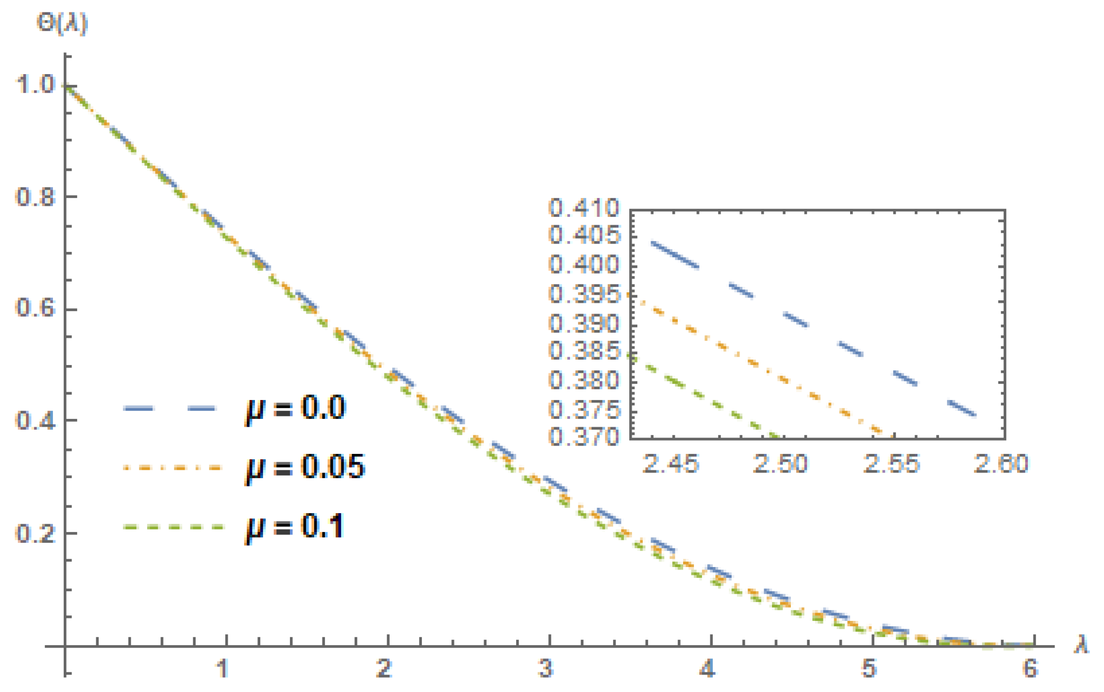
• With the heat source parameter $\epsilon$, the temperature profile $\Theta \left(\lambda \right)$ is observed to decrease for the case of pure water, Cu-water, and Ag-water. Thus, an increase in $\epsilon$ will cause a decrease in base fluid’s temperature, hence affecting the base fluid inversely. This also indicates that the internal heat of the nanofluid is more pronounced than that of the base fluid;
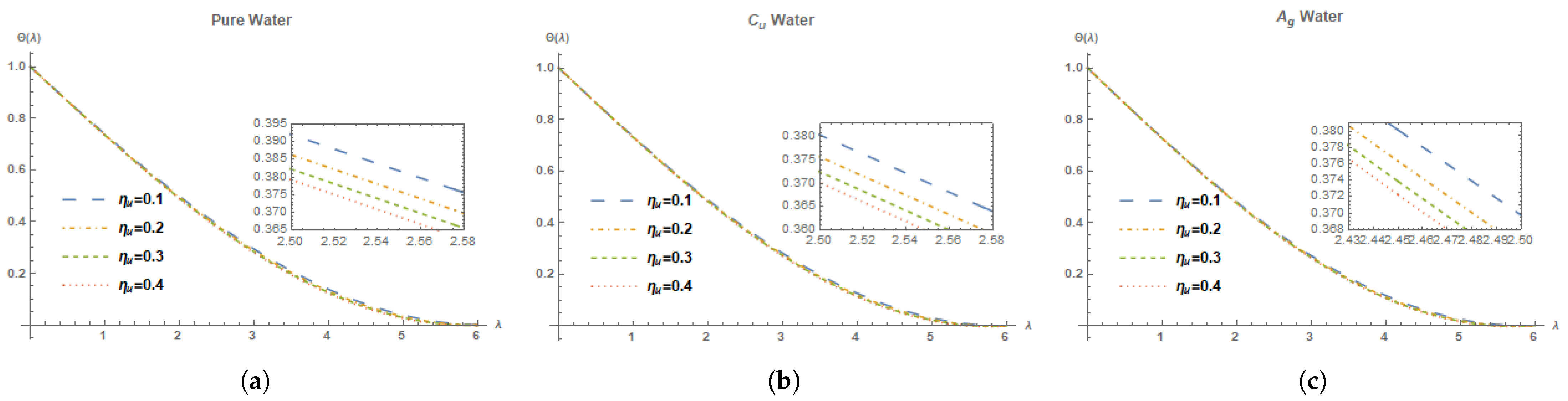
• For pure water, Cu-water, and Ag-water, the impact of volume fraction of nanoparticles is observed. The temperature profile $\Theta \left(\lambda \right)$ is seen to be decreased with constant magnetic field with the increase in volume fraction. Thus, an increase/decrease in $\mu$ caused an increase/decrease in the nanofluid’s temperature. This also confirms the notion that the thermal conductivity of the nanofluid is strongly dependent on the nanoparticle volume fraction;
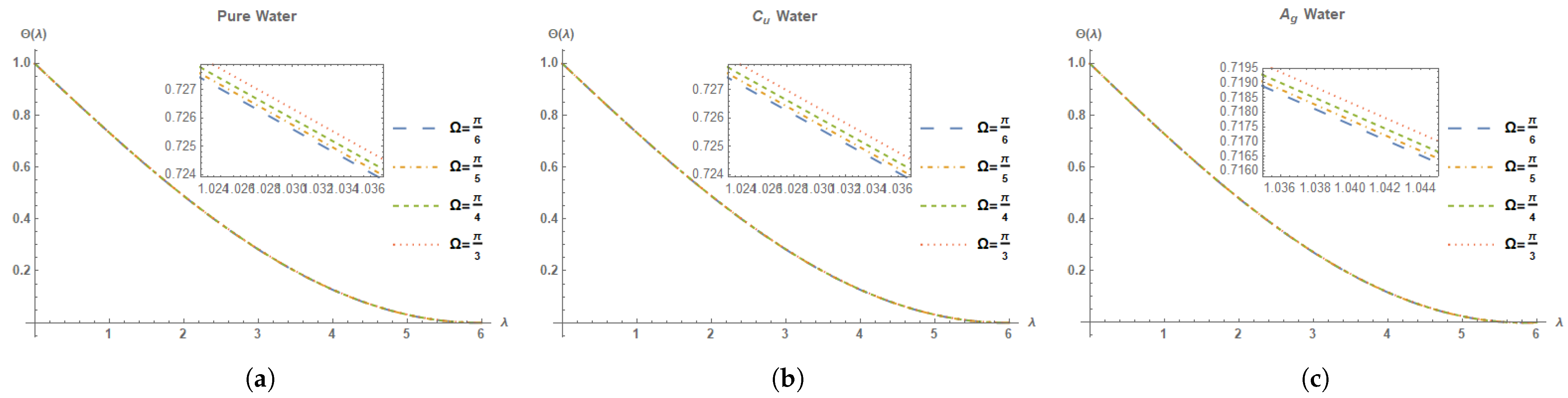
• For the wedge angle $\chi$, the temperature profile $\Theta \left(\lambda \right)$ is observed to increase in case of pure-water, Cu-water, and Ag-water. Thus, an increase or decrease in angle of wedge $\chi$ can cause an increase or decrease in the base fluid temperature. The results indicated that Cu and Ag water heated fast for $\chi$, and this is due to high angle of inclination;
• The velocity profile $h^{\prime }\left(\lambda \right)$ is also analyzed with variations in the unsteadiness ${\eta }_u$, stretching rate m parameters and angle of wedge $\chi$. Both ${\eta }_u$ and m parameters incited an increase for the case of pure water, Cu-water, and Ag-water. Thus, an increase or decrease in the ${\eta }_u$ and m parameters will cause an increase or decrease in the base fluid’s velocity. Decrease in velocity as increase in $\chi$ for the case of pure water, Cu-water, and Ag-water. Hence, mixing nanoparticles in nanofluid will have a considerable effect on liquid thermo-physical properties. Increasing trend is observed for pure water, Cu-water, and Ag-water for both m and ${\eta }_u$ and decreasing trend for $\chi$.

References

1. Bauer, N.; Rose, S.K.; Fujimori, S.; Van Vuuren, D.P.; Weyant, J.; Wise, M.; Cui, Y.; Daioglou, V.; Gidden, M.J.; Kato, E.; et al. Global energy sector emission reductions and bioenergy use: Overview of the bioenergy demand phase of the EMF-33 model comparison. Clim. Chang. 2020, 163, 1553–1568. [Google Scholar] [CrossRef]
2. Dincer, I. Renewable energy and sustainable development: A crucial review. Renew. Sustain. Energy Rev. 2000, 4, 157–175. [Google Scholar] [CrossRef]
3. National Renewable Energy Laboratory (US). Assessment of Parabolic Trough and Power Tower Solar Technology Cost and Performance Forecasts; DIANE Publishing: Pennsylvania, PA, USA, 2003; Volume 550. [Google Scholar]
4. Thi, N.D.A. The Evolution of Floating Solar Photovoltaics; Research Gate: Berlin, Germany, 2017. [Google Scholar]
5. Kim, S.; Bang, I.C.; Buongiorno, J.; Hu, L. Study of pool boiling and critical heat flux enhancement in nanofluids. Bull. Pol. Acad. Sci. Tech. Sci. 2007, 55, 211–216. [Google Scholar]
6. Kim, S.J.; Bang, I.C.; Buongiorno, J.; Hu, L. Surface wettability change during pool boiling of nanofluids and its effect on critical heat flux. Int. J. Heat Mass Transf. 2007, 50, 4105–4116. [Google Scholar] [CrossRef]
7. Han, Z.; Cao, F.; Yang, B. Synthesis and thermal characterization of phase-changeable indium/polyalphaolefin nanofluids. Appl. Phys. Lett. 2008, 92, 243104. [Google Scholar] [CrossRef]
8. Buongiorno, J.; Hu, L.W.; Kim, S.J.; Hannink, R.; Truong, B.; Forrest, E. Nanofluids for enhanced economics and safety of nuclear reactors: An evaluation of the potential features, issues, and research gaps. Nucl. Technol. 2008, 162, 80–91. [Google Scholar] [CrossRef]
9. Routbort, J. Argonne National Lab, Michellin North America, St. 2009. Available online: http://www1.eere.energy.gov/industry/nanomanufacturing/pdfs/nanofluidsindustrialcooling.pdf (accessed on 15 November 2021).
10. Donzelli, G.; Cerbino, R.; Vailati, A. Bistable heat transfer in a nanofluid. Phys. Rev. Lett. 2009, 102, 104503. [Google Scholar] [CrossRef]
11. Ghalambaz, M.; Groşan, T.; Pop, I. Mixed convection boundary layer flow and heat transfer over a vertical plate embedded in a porous medium filled with a suspension of nano-encapsulated phase change materials. J. Mol. Liq. 2019, 293, 111432. [Google Scholar] [CrossRef]
12. Ghalambaz, M.; Chamkha, A.J.; Wen, D. Natural convective flow and heat transfer of nano-encapsulated phase change materials (NEPCMs) in a cavity. Int. J. Heat Mass Transf. 2019, 138, 738–749. [Google Scholar] [CrossRef]
13. Navarrete, N.; Mondragón, R.; Wen, D.; Navarro, M.E.; Ding, Y.; Juliá, J.E. Thermal energy storage of molten salt–based nanofluid containing nano-encapsulated metal alloy phase change materials. Energy 2019, 167, 912–920. [Google Scholar] [CrossRef] [Green Version]
14. Ahmadi, M.H.; Mirlohi, A.; Nazari, M.A.; Ghasempour, R. A review of thermal conductivity of various nanofluids. J. Mol. Liq. 2018, 265, 181–188. [Google Scholar] [CrossRef]
15. Ekechukwu, O.; Norton, B. Review of solar-energy drying systems III: Low temperature air-heating solar collectors for crop drying applications. Energy Convers. Manag. 1999, 40, 657–667. [Google Scholar] [CrossRef]
16. Peng, D.; Zhang, X.; Dong, H.; Lv, K. Performance study of a novel solar air collector. Appl. Therm. Eng. 2010, 30, 2594–2601. [Google Scholar] [CrossRef]
17. Kandasamy, R.; Loganathan, P.; Arasu, P.P. Scaling group transformation for MHD boundary-layer flow of a nanofluid past a vertical stretching surface in the presence of suction/injection. Nucl. Eng. Des. 2011, 241, 2053–2059. [Google Scholar] [CrossRef] [Green Version]
18. Vajravelu, K.; Prasad, K.; Lee, J.; Lee, C.; Pop, I.; Van Gorder, R.A. Convective heat transfer in the flow of viscous Ag–water and Cu–water nanofluids over a stretching surface. Int. J. Therm. Sci. 2011, 50, 843–851. [Google Scholar] [CrossRef]
19. Al-Oran, O.; Lezsovits, F. A Hybrid Nanofluid of Alumina and Tungsten Oxide for Performance Enhancement of a Parabolic Trough Collector under the Weather Conditions of Budapest. Appl. Sci. 2021, 11, 4946. [Google Scholar] [CrossRef]
20. Rana, P.; Bhargava, R. Numerical study of heat transfer enhancement in mixed convection flow along a vertical plate with heat source/sink utilizing nanofluids. Commun. Nonlinear Sci. Numer. Simul. 2011, 16, 4318–4334. [Google Scholar] [CrossRef]
21. Ahmad, S.; Rohni, A.M.; Pop, I. Blasius and Sakiadis problems in nanofluids. Acta Mech. 2011, 218, 195–204. [Google Scholar] [CrossRef]
22. Yacob, N.A.; Ishak, A.; Pop, I. Falkner–Skan problem for a static or moving wedge in nanofluids. Int. J. Therm. Sci. 2011, 50, 133–139. [Google Scholar] [CrossRef]
23. Hamad, M. Analytical solution of natural convection flow of a nanofluid over a linearly stretching sheet in the presence of magnetic field. Int. Commun. Heat Mass Transf. 2011, 38, 487–492. [Google Scholar] [CrossRef]
24. Magyari, E. Comment on the homogeneous nanofluid models applied to convective heat transfer problems. Acta Mech. 2011, 222, 381–385. [Google Scholar] [CrossRef]
25. Wang, Y.; Xu, J.; Liu, Q.; Chen, Y.; Liu, H. Performance analysis of a parabolic trough solar collector using Al2O3/synthetic oil nanofluid. Appl. Therm. Eng. 2016, 107, 469–478. [Google Scholar] [CrossRef]
26. Olia, H.; Torabi, M.; Bahiraei, M.; Ahmadi, M.H.; Goodarzi, M.; Safaei, M.R. Application of nanofluids in thermal performance enhancement of parabolic trough solar collector: State-of-the-art. Appl. Sci. 2019, 9, 463. [Google Scholar] [CrossRef] [Green Version]
27. Moravej, M.; Bozorg, M.V.; Guan, Y.; Li, L.K.; Doranehgard, M.H.; Hong, K.; Xiong, Q. Enhancing the efficiency of a symmetric flat-plate solar collector via the use of rutile TiO2-water nanofluids. Sustain. Energy Technol. Assess. 2020, 40, 100783. [Google Scholar] [CrossRef]
28. Taherian, H.; Rezania, A.; Sadeghi, S.; Ganji, D. Experimental validation of dynamic simulation of the flat plate collector in a closed thermosyphon solar water heater. Energy Convers. Manag. 2011, 52, 301–307. [Google Scholar] [CrossRef]
29. Yousefi, T.; Veysi, F.; Shojaeizadeh, E.; Zinadini, S. An experimental investigation on the effect of Al2O3–H2O nanofluid on the efficiency of flat-plate solar collectors. Renew. Energy 2012, 39, 293–298. [Google Scholar] [CrossRef]
30. Javadi, F.S.; Saidur, R.; Kamalisarvestani, M. Investigating performance improvement of solar collectors by using nanofluids. Renew. Sustain. Energy Rev. 2013, 28, 232–245. [Google Scholar] [CrossRef]
31. Faizal, M.; Saidur, R.; Mekhilef, S.; Alim, M.A. Energy, economic and environmental analysis of metal oxides nanofluid for flat-plate solar collector. Energy Convers. Manag. 2013, 76, 162–168. [Google Scholar] [CrossRef]
32. Liu, Z.H.; Hu, R.L.; Lu, L.; Zhao, F.; Xiao, H.s. Thermal performance of an open thermosyphon using nanofluid for evacuated tubular high temperature air solar collector. Energy Convers. Manag. 2013, 73, 135–143. [Google Scholar] [CrossRef]
33. Hawwash, A.; Rahman, A.K.A.; Nada, S.; Ookawara, S. Numerical investigation and experimental verification of performance enhancement of flat plate solar collector using nanofluids. Appl. Therm. Eng. 2018, 130, 363–374. [Google Scholar] [CrossRef]
34. Tayebi, R.; Akbarzadeh, S.; Valipour, M.S. Numerical investigation of efficiency enhancement in a direct absorption parabolic trough collector occupied by a porous medium and saturated by a nanofluid. Environ. Prog. Sustain. Energy 2019, 38, 727–740. [Google Scholar] [CrossRef]
35. Sheikholeslami, M.; Farshad, S.A.; Ebrahimpour, Z.; Said, Z. Recent progress on flat plate solar collectors and photovoltaic systems in the presence of nanofluid: A review. J. Clean. Prod. 2021, 293, 126119. [Google Scholar] [CrossRef]
36. Shoaib, M.; Raja, M.A.Z.; Sabir, M.T.; Islam, S.; Shah, Z.; Kumam, P.; Alrabaiah, H. Numerical investigation for rotating flow of MHD hybrid nanofluid with thermal radiation over a stretching sheet. Sci. Rep. 2020, 10, 1–15. [Google Scholar]
37. Fudholi, A.; Sopian, K.; Othman, M.Y.; Ruslan, M.H.; Bakhtyar, B. Energy analysis and improvement potential of finned double-pass solar collector. Energy Convers. Manag. 2013, 75, 234–240. [Google Scholar] [CrossRef]
38. Mushtaq, A.; Mustafa, M.; Hayat, T.; Alsaedi, A. Nonlinear radiative heat transfer in the flow of nanofluid due to solar energy: A numerical study. J. Taiwan Inst. Chem. Eng. 2014, 45, 1176–1183. [Google Scholar] [CrossRef]
39. Javed, A.; Iqbal, S.; Hashmi, M.S.; Dar, A.H.; Khan, N. Semi-analytical solutions of nonlinear problems of the deformation of beams and of the plate deflection theory using the optimal homotopy asymptotic method. Heat Transf. Res. 2014, 45, 603–620. [Google Scholar] [CrossRef]
40. Iqbal, S.; Hashmi, M.S.; Khan, N.; Ramzan, M.; Dar, A.H. Numerical solutions of telegraph equations using an optimal homotopy asymptotic method. Heat Transf. Res. 2015, 46, 699–712. [Google Scholar] [CrossRef]
41. Sarwar, F.; Iqbal, S. Use of optimal homotopy asymptotic method for fractional order nonlinear fredholm integro-differential equations. Sci. Int. 2015, 27, 3033–3040. [Google Scholar]
42. Mufti, M.R.; Qureshi, M.I.; Alkhalaf, S.; Iqbal, S. An Algorithm: Optimal Homotopy Asymptotic Method for Solutions of Systems of Second-Order Boundary Value Problems. Math. Probl. Eng. 2017, 2017, 8013164. [Google Scholar] [CrossRef] [Green Version]
43. Iqbal, S.; Idrees, M.; Siddiqui, A.M.; Ansari, A.R. Some solutions of the linear and nonlinear Klein–Gordon equations using the optimal homotopy asymptotic method. Appl. Math. Comput. 2010, 216, 2898–2909. [Google Scholar] [CrossRef]
44. Vafai, K.; Alkire, R.; Tien, C. An experimental investigation of heat transfer in variable porosity media. J. Heat Transf. 1985, 107, 642–647. [Google Scholar] [CrossRef]
45. Tien, C.; Hong, J. Natural convection in porous media under non-Darcian and non-uniform permeability conditions. In Natural Convection: Fundamentals and Applications; Hemisphere Publishing: London, UK, 1985. [Google Scholar]
46. Fathalah, K.; Elsayed, M. Natural convection due to solar radiation over a non-absorbing plate with and without heat losses. Int. J. Heat Fluid Flow 1980, 2, 41–45. [Google Scholar] [CrossRef]
47. Oztop, H.F.; Abu-Nada, E. Numerical study of natural convection in partially heated rectangular enclosures filled with nanofluids. Int. J. Heat Fluid Flow 2008, 29, 1326–1336. [Google Scholar] [CrossRef]
48. Mohamad, R.B.; Kandasamy, R.; Muhaimin, I. Enhance of heat transfer on unsteady Hiemenz flow of nanofluid over a porous wedge with heat source/sink due to solar energy radiation with variable stream condition. Heat Mass Transf. 2013, 49, 1261–1269. [Google Scholar] [CrossRef] [Green Version]
49. Sattar, M. A local similarity transformation for the unsteady two-dimensional hydrodynamic boundary layer equations of a flow past a wedge. Int. J. Appl. Math. Mech 2011, 7, 15–28. [Google Scholar]
50. Raptis, A. Radiation and free convection flow through a porous medium. Int. Commun. Heat Mass Transf. 1998, 25, 289–295. [Google Scholar] [CrossRef]
51. Kafoussias, N.; Nanousis, N. Magnetohydrodynamic laminar boundary-layer flow over a wedge with suction or injection. Can. J. Phys. 1997, 75, 733–745. [Google Scholar] [CrossRef]
52. Marinca, V.; Herişanu, N. Determination of periodic solutions for the motion of a particle on a rotating parabola by means of the optimal homotopy asymptotic method. J. Sound Vib. 2010, 329, 1450–1459. [Google Scholar] [CrossRef]
53. Marinca, V.; Herişanu, N. Application of Optimal Homotopy Asymptotic Method for solving nonlinear equations arising in heat transfer. Int. Commun. Heat Mass Transf. 2008, 35, 710–715. [Google Scholar] [CrossRef]
54. Zeb, A.; Iqbal, S.; Siddiqui, A.; Haroon, T. Application of the optimal homotopy asymptotic method to flow with heat transfer of a pseudoplastic fluid inside a circular pipe. J. Chin. Inst. Eng. 2013, 36, 797–805. [Google Scholar] [CrossRef]
55. Lu, J. Variational iteration method for solving a nonlinear system of second-order boundary value problems. Comput. Math. Appl. 2007, 54, 1133–1138. [Google Scholar] [CrossRef] [Green Version]
56. Saadatmandi, A.; Dehghan, M.; Eftekhari, A. Application of He’s homotopy perturbation method for non-linear system of second-order boundary value problems. Nonlinear Anal. Real World Appl. 2009, 10, 1912–1922. [Google Scholar] [CrossRef]
Figure 1. Flow model over a porous wedge sheet.
Applsci 11 10855 g001
Figure 2. Schematic representation for the MHD Hiemenz flow analysis of nanofluid over a porous wedge.
Applsci 11 10855 g002
Figure 3. Temperature profile Θ ( λ ) for different choices of magnetic filed parameter M at N = 0.5 , m = 1 , P R = 6 , χ = π 6 , τ = 0.6 , η u = 0.1 , Γ = 2 , ε = 1 , C T = 0.1 , S = 1 showing their exciting nature. (a) pure-water. (b) Cu-water. (c) Ag-water.
Applsci 11 10855 g003
Figure 4. Temperature profile Θ ( λ ) for different choices of conductive radiation parameter N at M = 9 , m = 1 , P R = 6 , χ = π 6 , τ = 0.6 , η u = 0.1 , Γ = 2 , ε = 1 , C T = 0.1 , S = 1 showing their exciting nature. (a) pure-water. (b) Cu-water. (c) Ag-water.
Applsci 11 10855 g004
Figure 5. Temperature profile Θ ( λ ) for different choices of m at M = 9 , N = 0.5 , P R = 6 , χ = π 6 , τ = 0.6 , η u = 0.1 , Γ = 2 , ε = 1 , C T = 0.1 , S = 1 showing their exciting nature. (a) pure-water. (b) Cu-water. (c) Ag-water.
Applsci 11 10855 g005
Figure 6. Temperature profile Θ ( η ) for different choices of energy absorption elements μ at M = 9 , N = 0.5 , P R = 6 , χ = π 6 , τ = 0.6 , η u = 0.1 , Γ = 2 , ε = 1 , C T = 0.1 , S = 1 showing their exciting nature.
Applsci 11 10855 g006
Figure 7. Temperature profile Θ ( λ ) for different choices of unsteadiness parameter η u at M = 9 , N = 0.5 , P R = 6 , χ = π 6 , τ = 0.6 , Γ = 2 , ε = 1 , C T = 0.1 , S = 1 showing their exciting nature. (a) pure-water. (b) Cu-water. (c) Ag-water.
Applsci 11 10855 g007
Figure 8. Temperature profile Θ ( λ ) for different choices of heat source/sink parameter ε at M = 9 , N = 0.5 , P R = 6 , χ = π 6 , τ = 0.6 , η u = 0.1 , Γ = 2 , ε = 1 , C T = 0.1 , S = 1 showing their exciting nature. (a) pure-water. (b) Cu-water. (c) Ag-water.
Applsci 11 10855 g008
Figure 9. Temperature profile Θ ( λ ) for different choices of angle of wedge χ at M = 9 , N = 0.5 , P R = 6 , ε = 1 , τ = 0.6 , η u = 0.1 , Γ = 2 , ε = 1 , C T = 0.1 , S = 1 showing their exciting nature. (a) pure-water. (b) Cu-water. (c) Ag-water.
Applsci 11 10855 g009
Figure 10. Velocity profile h ( λ ) for different choices of unsteadiness parameter η u at M = 9 , N = 0.5 , P R = 6 , χ = π 6 , τ = 0.6 , Γ = 2 , ε = 1 , C T = 0.1 , S = 1 showing their exciting nature. (a) pure-water. (b) Cu-water. (c) Ag-water.
Applsci 11 10855 g010
Figure 11. Velocity profile h ( λ ) for different choices of m at M = 9 , N = 0.5 , P R = 6 , χ = π 6 , τ = 0.6 , Γ = 2 , ε = 1 , C T = 0.1 , S = 1 showing their exciting nature. (a) pure-water. (b) Cu-water. (c) Ag-water.
Applsci 11 10855 g011
Figure 12. Velocity profile h ( λ ) for different choices of χ at M = 9 , N = 0.5 , P R = 6 , τ = 0.6 , Γ = 2 , ε = 1 , C T = 0.1 , S = 1 showing their exciting nature. (a) pure-water. (b) Cu-water. (c) Ag-water.
Applsci 11 10855 g012