
A Novel Feature Selection Based on VMD and Information Gain for Pipe Blockages

Abstract
:1. Introduction
2. Materials and Methods
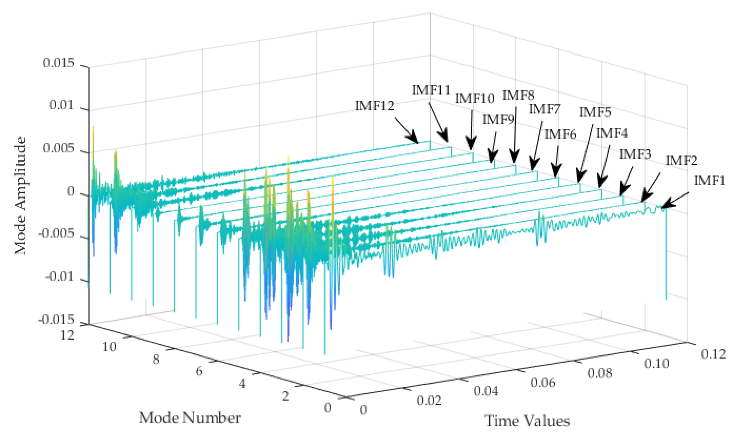
2.1. VMD
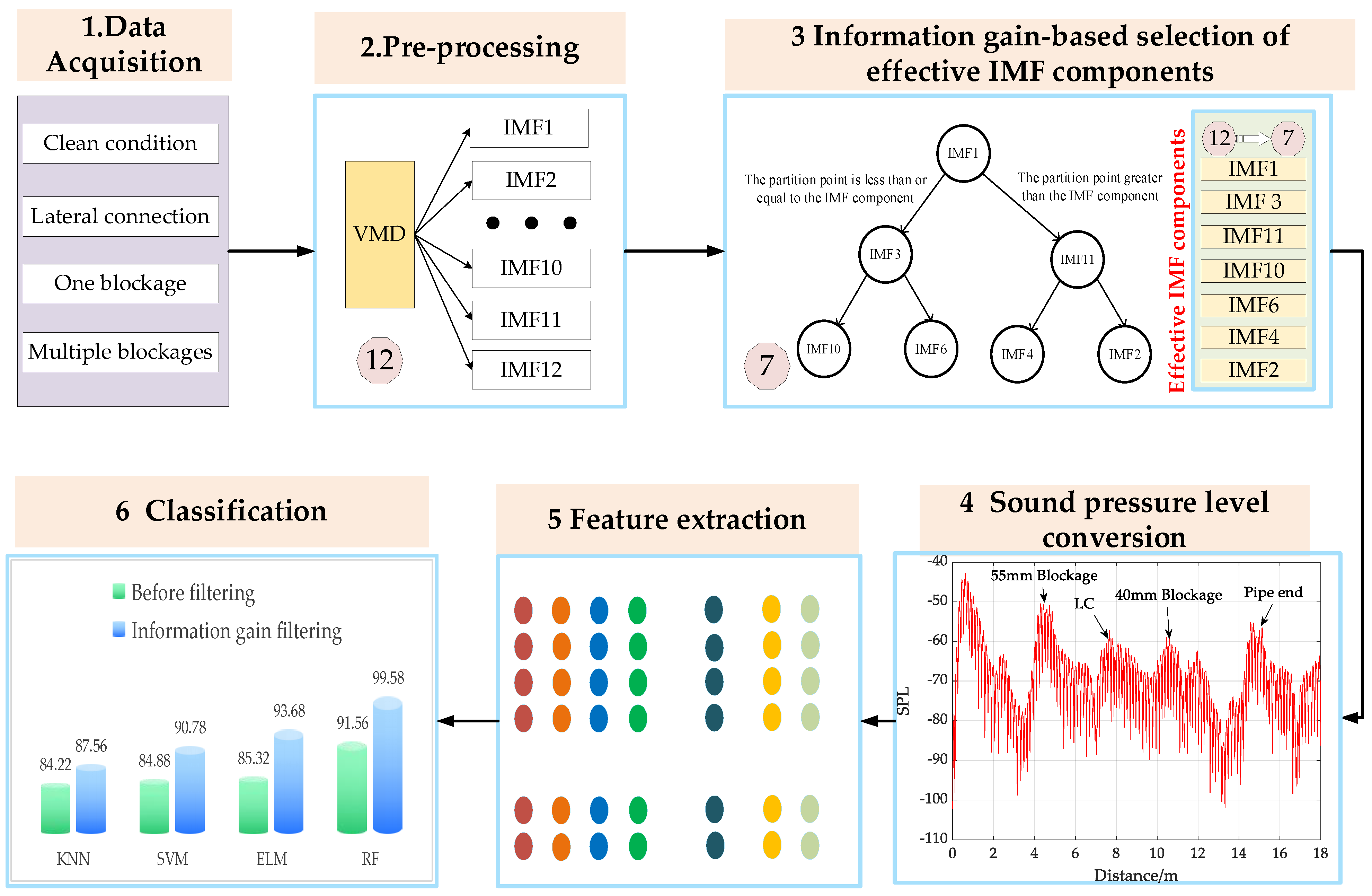
2.2. Information Gain-Based Selection of Effective IMF Components
2.3. Sound Pressure Level Conversion
2.4. RMSE
2.5. Proposed Feature Extraction Method
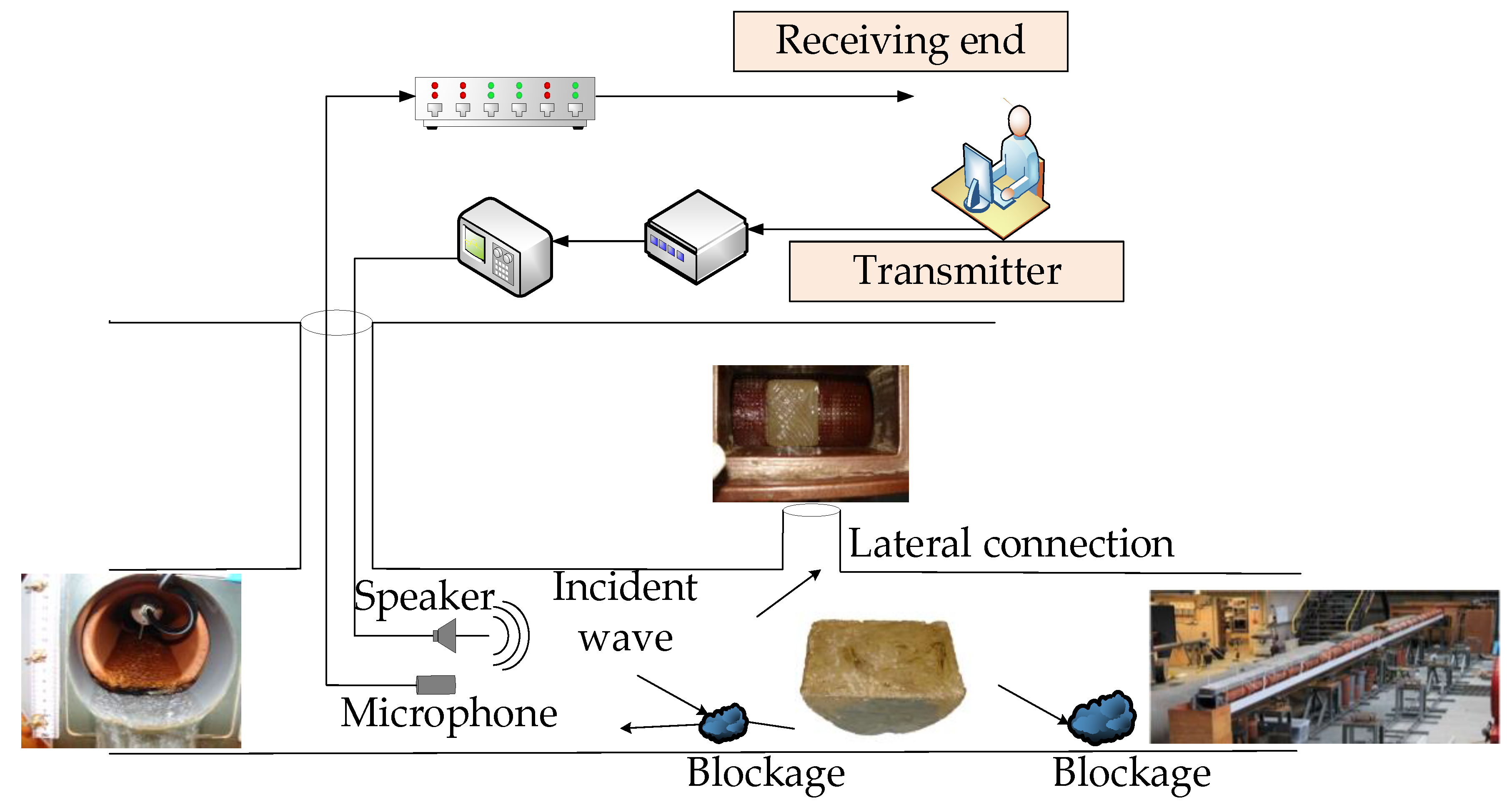
3. Experimental Setup and Experiment Conditions
4. Experimental Results and Analyses
4.1. Data Pre-Processing
4.2. Sensitive IMF Selection
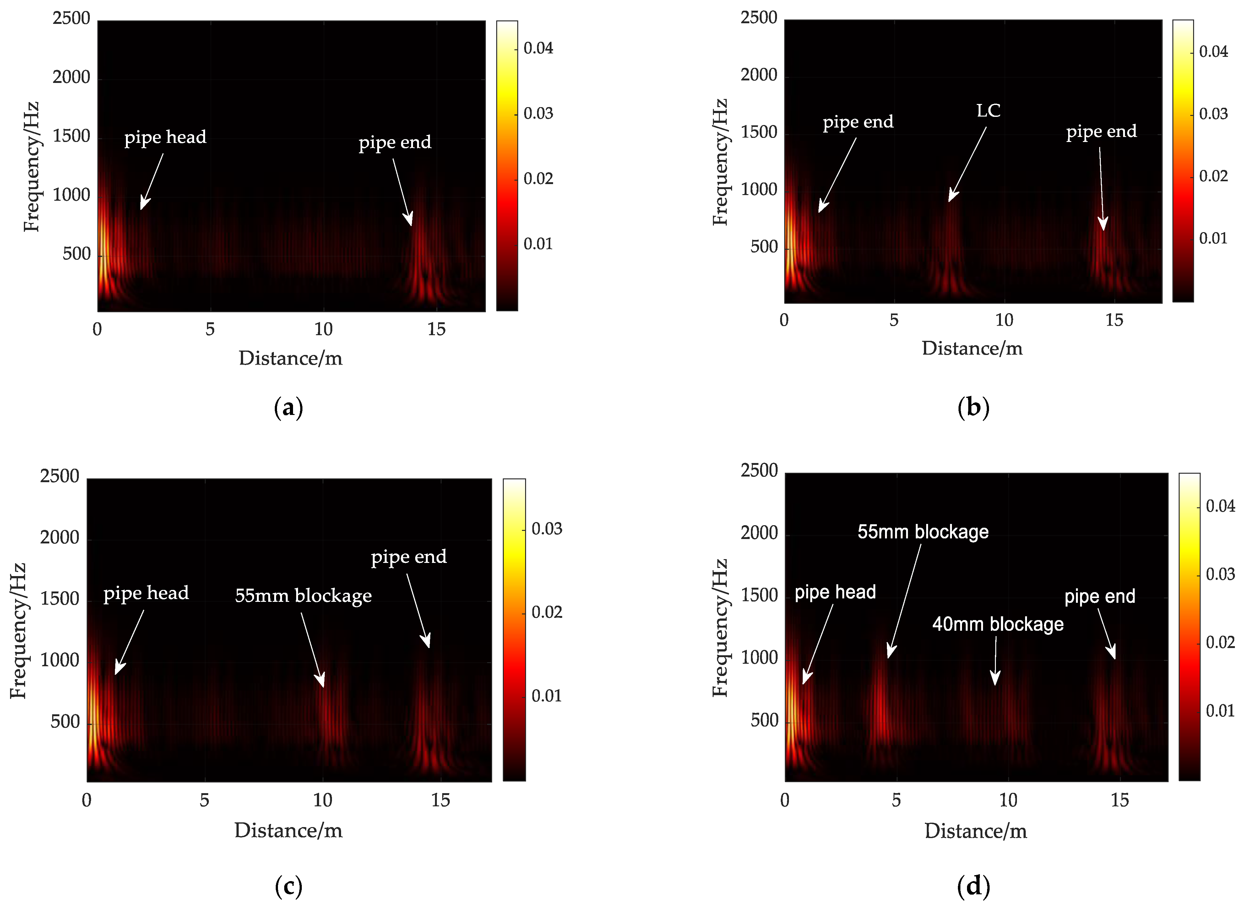
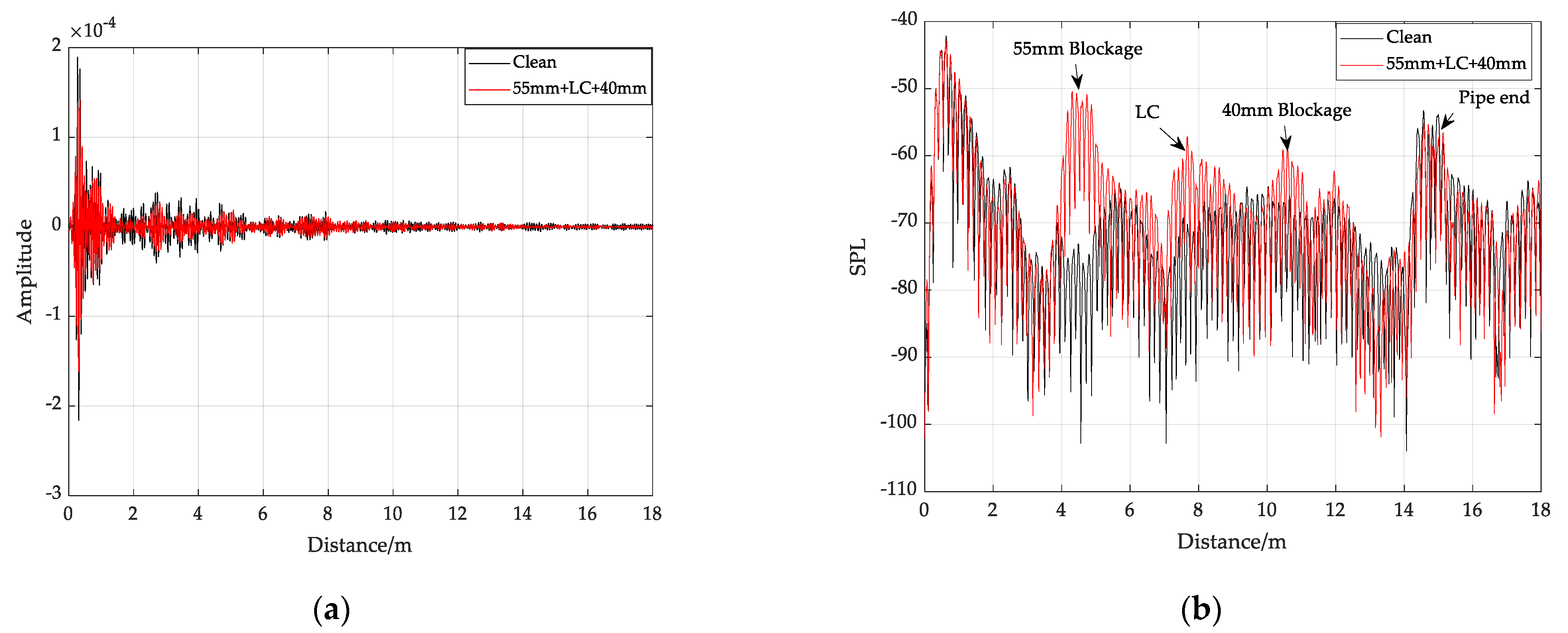
4.3. Sound Pressure Level Conversion
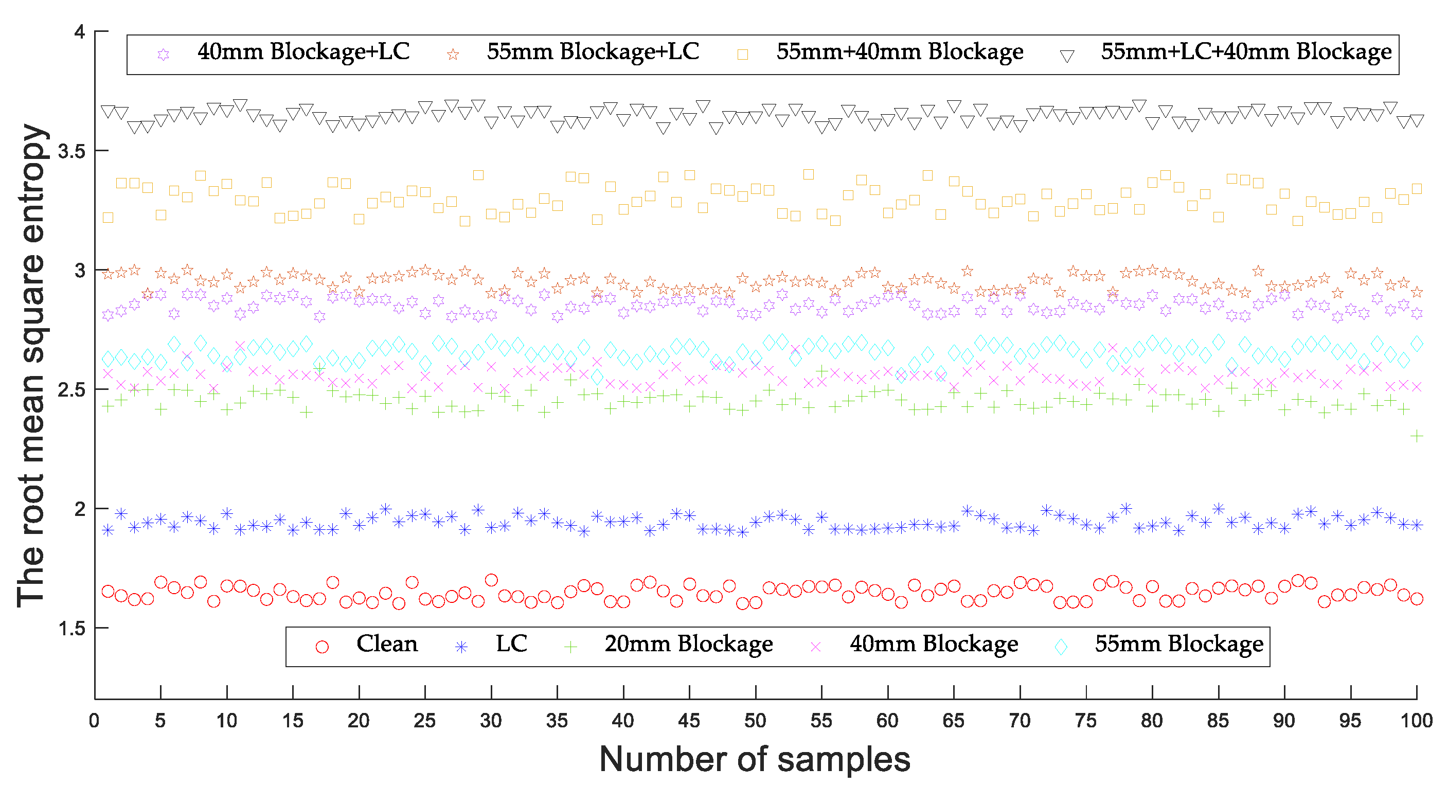
4.4. RMS Entropy Features Extraction and Blockage Recognition
5. Conclusions
Author Contributions
Funding
Institutional Review Board Statement
Informed Consent Statement
Data Availability Statement
Acknowledgments
Conflicts of Interest
References
- Zischg, J.; Rauch, W.; Sitzenfrei, R. Morphogenesis of urban water distribution networks: A spatiotemporal planning approach for cost-efficient and reliable supply. Entropy 2018, 20, 708. [Google Scholar] [CrossRef] [Green Version]
- Fathy, I.; Abdel-Aal, G.M.; Fahmy, M.R.; Fathy, A.; Zeleňáková, M. The Negative Impact of Blockage on Storm Water Drainage Network. Water 2020, 12, 1974. [Google Scholar] [CrossRef]
- Tu, M.-C.; Traver, R. Clogging Impacts on Distribution Pipe Delivery of Street Runoff to an Infiltration Bed. Water 2018, 10, 1045. [Google Scholar] [CrossRef] [Green Version]
- Pan, G.; Zheng, Y.; Guo, S.; Lv, Y. Automatic sewer pipe defect semantic segmentation based on improved U-Net. Autom. Constr. 2020, 119, 103383. [Google Scholar] [CrossRef]
- Sen, D.; Aghazadeh, A.; Mousavi, A.; Nagarajaiah, S.; Baraniuk, R.; Dabak, A. Data-driven semi-supervised and supervised learning algorithms for health monitoring of pipes. Mech. Syst. Signal Process. 2019, 131, 524–537. [Google Scholar] [CrossRef]
- Chi, Y.M.; Panda, A.; Byun, G.; Smith, C.F.; Lowe, K.T. Non-intrusive optical measurements of gas turbine engine inlet condensation using machine learning. Meas. Sci. Technol. 2021, 32, 044001. [Google Scholar]
- Datta, S.; Sarkar, S. A review on different pipeline fault detection methods. J. Loss Prev. Process. Ind. 2016, 41, 97–106. [Google Scholar] [CrossRef]
- Guan, R.; Lu, Y.; Duan, W.; Wang, X. Guided waves for damage identification in pipeline structures: A review. Struct. Control. Health Monit. 2017, 24, e2007. [Google Scholar] [CrossRef]
- Wang, M.; Luo, H.; Cheng, J.C. Towards an automated condition assessment framework of underground sewer pipes based on closed-circuit television (CCTV) images. Tunn. Undergr. Space Technol. 2021, 110, 103840. [Google Scholar] [CrossRef]
- Son, B.J.; Cho, T. Modified Crack Detection of Sewer Conduit with Low-Resolution Images. Appl. Sci. 2021, 11, 2263. [Google Scholar] [CrossRef]
- Haurum, J.B.; Moeslund, T.B. A Survey on Image-Based Automation of CCTV and SSET Sewer Inspections. Autom. Constr. 2020, 111, 103061. [Google Scholar] [CrossRef]
- Bin Ali, M.T.; Horoshenkov, K.V.; Tait, S.J. Rapid detection of sewer defects and blockages using acoustic-based instrumentation. Water Sci. Technol. 2011, 64, 1700–1707. [Google Scholar] [CrossRef] [PubMed]
- Khan, M.S. Empirical Modeling of Acoustic Signal Attenuation in Municipal Sewer Pipes for Condition Monitoring Applications. In Proceedings of the 2018 IEEE Green Technologies Conference (GreenTech), Austin, TX, USA, 4–6 April 2018; pp. 137–143. [Google Scholar]
- Kim, K.; Wang, S.; Ryu, H.; Lee, S.Q. Acoustic-Based Position Estimation of an Object and a Person Using Active Localization and Sound Field Analysis. Appl. Sci. 2020, 10, 9090. [Google Scholar] [CrossRef]
- Che, T.C.; Duan, H.F.; Lee, P.J. Transient wave-based methods for anomaly detection in fluid pipes: A review. Mech. Syst. Signal Process. 2021, 160, 107874. [Google Scholar] [CrossRef]
- Zeng, W.; Zecchin, A.C.; Gong, J.; Lambert, M.F.; Cazzolato, B.S. Inverse Wave Reflectometry Method for Hydraulic Transient-Based Pipeline Condition Assessment. J. Hydraul. Eng. 2020, 146, 04020056. [Google Scholar] [CrossRef]
- Hawari, A.; Alkadour, F.; Elmasry, M.; Zayed, T. A state of the art review on condition assessment models developed for sewer pipelines. Eng. Appl. Artif. Intell. 2020, 93, 103721. [Google Scholar] [CrossRef]
- Singh, D.; Singh, B. Hybridization of feature selection and feature weighting for high dimensional data. Appl. Intell. 2018, 49, 1580–1596. [Google Scholar] [CrossRef]
- Bayat, M.; Ahmadi, H.R.; Mahdavi, N. Application of power spectral density function for damage diagnosis of bridge piers. Struct. Eng. Mech. 2019, 71, 57–63. [Google Scholar]
- Ahmadi, H.R.; Mahdavi, N.; Bayat, M. A novel damage identification method based on short time Fourier transform and a new efficient index. Structures 2021, 33, 3605–3614. [Google Scholar] [CrossRef]
- Xu, C.; Du, S.; Gong, P.; Li, Z.; Chen, G.; Song, G. An Improved Method for Pipeline Leakage Localization With a Single Sensor Based on Modal Acoustic Emission and Empirical Mode Decomposition With Hilbert Transform. IEEE Sens. J. 2020, 20, 5480–5491. [Google Scholar] [CrossRef]
- Sun, J.; Peng, Z.; Wen, J. Leakage Aperture Recognition based on Ensemble Local Mean Decomposition and Sparse Representation for Classification of Natural Gas Pipeline. Measurement 2017, 108, 91–100. [Google Scholar] [CrossRef]
- Jiang, L.; Ma, Z.; Zhang, J.; Khan, M.Y.A.; Cheng, M.; Wang, L. Chaotic Characteristic Analysis of Vibration Response of Pumping Station Pipeline Using Improved Variational Mode Decomposition Method. Appl. Sci. 2021, 11, 8864. [Google Scholar] [CrossRef]
- Fu, L.; Zhu, T.; Pan, G.; Chen, S.; Wei, Y. Power Quality Disturbance Recognition Using VMD-Based Feature Extraction and Heuristic Feature Selection. Appl. Sci. 2019, 9, 4901. [Google Scholar] [CrossRef] [Green Version]
- Sun, J.; Xiao, Q.; Wen, J.; Zhang, Y. Natural gas pipeline leak aperture identification and location based on local mean decomposition analysis. Measurement 2016, 79, 147–157. [Google Scholar] [CrossRef]
- Lee, P.J.; Duan, H.; Tuck, J.; Ghidaoui, M. Numerical and Experimental Study on the Effect of Signal Bandwidth on Pipe Assessment Using Fluid Transients. J. Hydraul. Eng. 2015, 141, 04014074. [Google Scholar] [CrossRef]
- Wenxuan, W.; Zhijian, W.; Jiping, Z.; Weijin, M.; Junyuan, W. Research of the Method of Determining k Value in VMD based on Kurtosis. J. Mech. Transm. 2018, 42, 153–160. [Google Scholar]
- Wang, B.; Li, Y.; Zhao, W.; Zhang, Z.; Zhang, Y.; Wang, Z. Effective Crack Damage Detection Using Multilayer Sparse Feature Representation and Incremental Extreme Learning Machine. Appl. Sci. 2019, 9, 614. [Google Scholar] [CrossRef] [Green Version]
- Azhagusundari, B.; Thanamani, A.S. Feature selection based on information gain. Int. J. Innov. Technol. Explor. Eng. (IJITEE) 2013, 2, 18–21. [Google Scholar]
- Deng, H.; Diao, Y.; Wu, W.; Zhang, J.; Zhong, X. A high-speed D-CART online fault diagnosis algorithm for rotor systems. Appl. Intell. 2019, 50, 29–41. [Google Scholar] [CrossRef]
- Dragomiretskiy, K.; Zosso, D. Variational Mode Decomposition. IEEE Trans. Signal Process. 2014, 62, 531–544. [Google Scholar] [CrossRef]
- Shi, H.; Fu, W.; Li, B.; Shao, K.; Yang, D. Intelligent Fault Identification for Rolling Bearings Fusing Average Refined Composite Multiscale Dispersion Entropy-Assisted Feature Extraction and SVM with Multi-Strategy Enhanced Swarm Optimization. Entropy 2021, 23, 527. [Google Scholar] [CrossRef] [PubMed]
- Kent, J.T. Information gain and a general measure of correlation. Biometrika 1983, 70, 163–173. [Google Scholar] [CrossRef]
- Younes, R.; Ouelaa, N.; Hamzaoui, N.; Djamaa, M.C.; Djebala, A. The Influence of the Sound Pressure Level on the Identification of the Defects Severity in Gear Transmission by the Sound Perception. Acoust. Aust. 2019, 47, 239–246. [Google Scholar] [CrossRef]
- Santo, F.T.; Sattar, T.P.; Edwards, G. Validation of Acoustic Emission Waveform Entropy as a Damage Identification Feature. Appl. Sci. 2019, 9, 4070. [Google Scholar] [CrossRef] [Green Version]
- Sharma, V.; Parey, A. Gearbox fault diagnosis using RMS based probability density function and entropy measures for fluctuating speed conditions. Struct. Health Monit. 2017, 16, 682–695. [Google Scholar] [CrossRef]
- Feng, Z. Condition Classification in Underground Pipes Based on Acoustical Characteristics. Ph.D. Thesis, University of Bradford, Bradford, UK, 2013. [Google Scholar]
- Zhu, X.; Huang, G.; Feng, Z.; Wu, J. Condition Classification of Water-Filled Underground Siphon Using Acoustic Sensors. Sensors 2019, 20, 186. [Google Scholar] [CrossRef] [Green Version]


| No | State | Pipe Condition | Training Samples | Testing Samples |
|---|---|---|---|---|
| 1 | normally | Clean | 200 | 100 |
| 2 | Lateral Connection (LC) | 200 | 100 | |
| 3 | single blockage | a 20 mm blockage | 200 | 100 |
| 4 | a 40 mm blockage | 200 | 100 | |
| 5 | a 50 mm blockage | 200 | 100 | |
| 6 | multiple blockages | a 40 mm blockage and a LC | 200 | 100 |
| 7 | a 55 mm blockage and a LC | 200 | 100 | |
| 8 | a 40 mm blockage and a 55 mm blockage | 200 | 100 | |
| 9 | a 40 mm blockage, a 55 mm blockage, and LC | 200 | 100 |
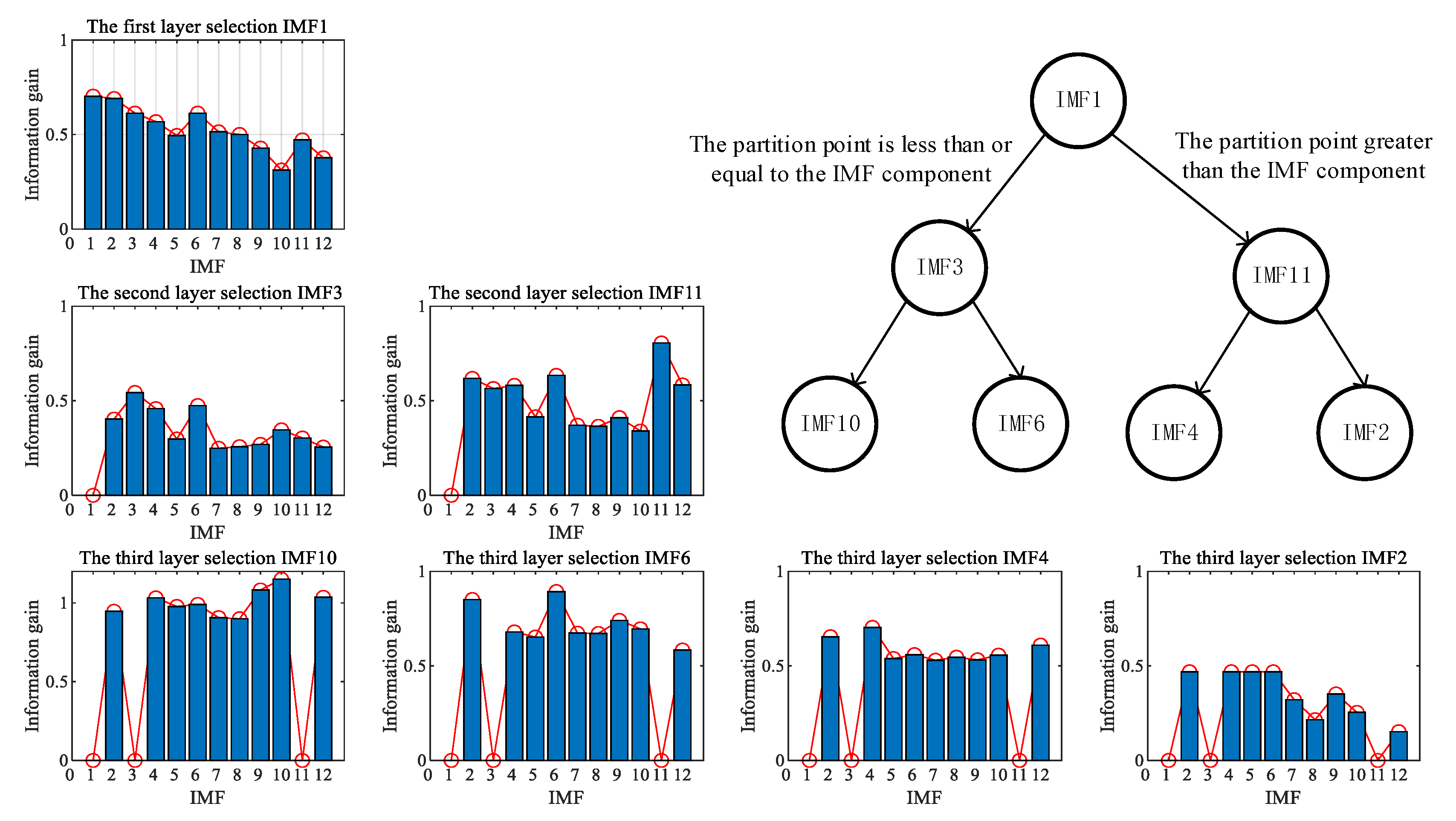
| Number of Layers | Screening of Sensitive IMF |
|---|---|
| The first layer selection IMF | IMF1; |
| The second layer selection IMF | IMF3; IMF11; |
| The second layer selection IMF | IMF10; IMF6; IMF4; IMF2; |
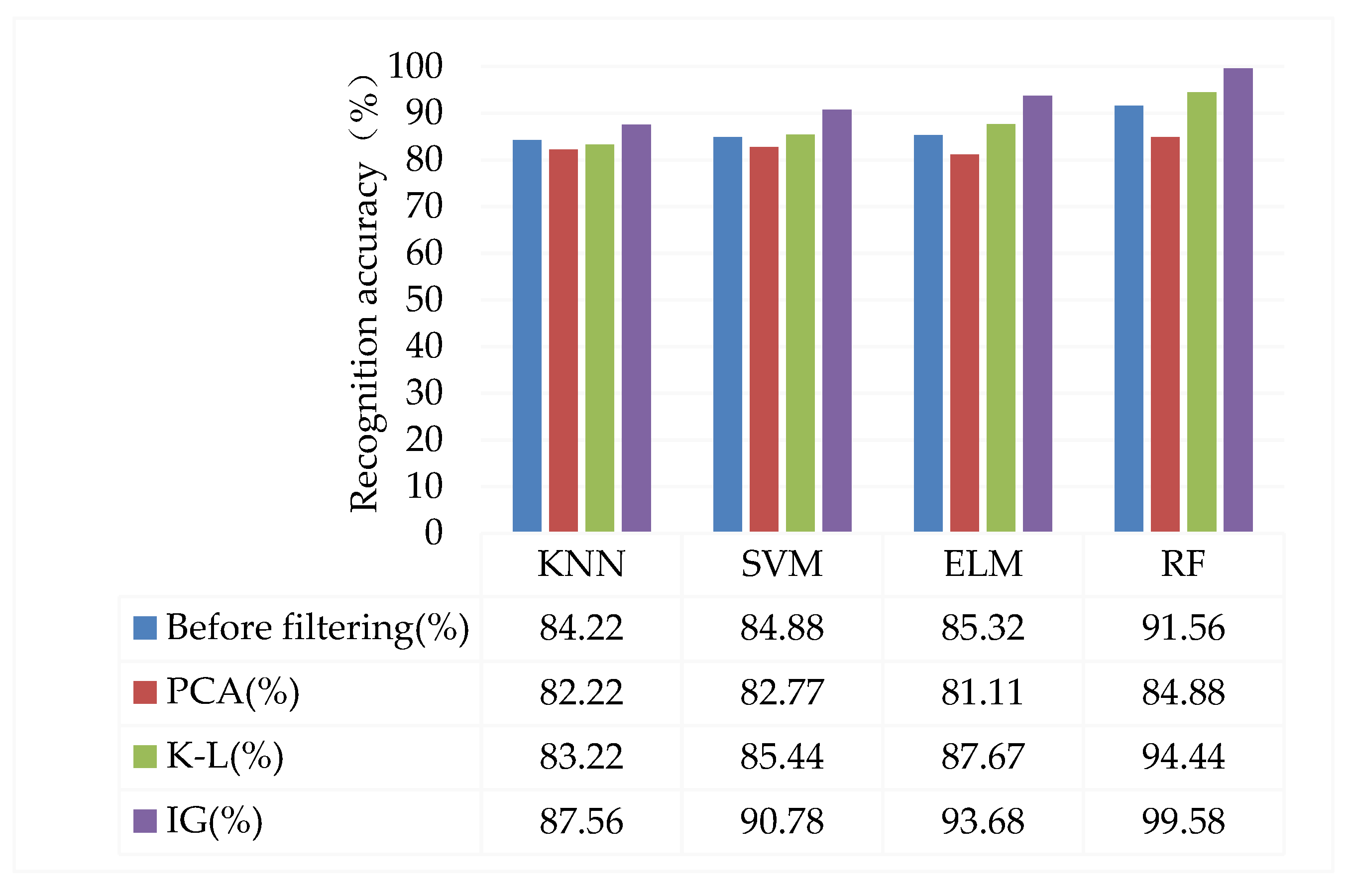
| Classifier | Max Accuracy (%) | Min Accuracy (%) | Average Accuracy (%) |
|---|---|---|---|
| KNN | 90.44 | 86.67 | 87.56 |
| SVM | 91.11 | 90.56 | 90.78 |
| ELM | 94.44 | 90.44 | 93.68 |
| RF | 100 | 98.77 | 99.58 |
| Feature Extraction Method | Identification Accuracy (%) | Average Identification Accuracy (%) | Standard Deviation | |||
|---|---|---|---|---|---|---|
| 1 | 2 | 3 | 4 | |||
| EMD-IG-RMSE-RF | 91.11 | 90.33 | 89.11 | 91.78 | 90.58 | 0.54 |
| LMD-IG-RMSE-RF | 80.14 | 82.13 | 80.31 | 82.52 | 81.28 | 0.21 |
| WT-IG-RMSE-RF | 86.13 | 84.13 | 85.13 | 86.78 | 85.32 | 0.14 |
| VMD-IG-RMSE-RF | 98.56 | 98.88 | 100 | 100 | 99.58 | 0.07 |
Publisher’s Note: MDPI stays neutral with regard to jurisdictional claims in published maps and institutional affiliations. |
© 2021 by the authors. Licensee MDPI, Basel, Switzerland. This article is an open access article distributed under the terms and conditions of the Creative Commons Attribution (CC BY) license (https://creativecommons.org/licenses/by/4.0/).
Share and Cite
Zhu, X.; Feng, Z.; Wu, J.; Deng, W. A Novel Feature Selection Based on VMD and Information Gain for Pipe Blockages. Appl. Sci. 2021, 11, 10824. https://doi.org/10.3390/app112210824
Zhu X, Feng Z, Wu J, Deng W. A Novel Feature Selection Based on VMD and Information Gain for Pipe Blockages. Applied Sciences. 2021; 11(22):10824. https://doi.org/10.3390/app112210824
Chicago/Turabian StyleZhu, Xuefeng, Zao Feng, Jiande Wu, and Weiquan Deng. 2021. "A Novel Feature Selection Based on VMD and Information Gain for Pipe Blockages" Applied Sciences 11, no. 22: 10824. https://doi.org/10.3390/app112210824
APA StyleZhu, X., Feng, Z., Wu, J., & Deng, W. (2021). A Novel Feature Selection Based on VMD and Information Gain for Pipe Blockages. Applied Sciences, 11(22), 10824. https://doi.org/10.3390/app112210824