
A Modified Wavenumber Algorithm of Multi-Layered Structures with Oblique Incidence Based on Full-Matrix Capture


Abstract
:1. Introduction
2. Method
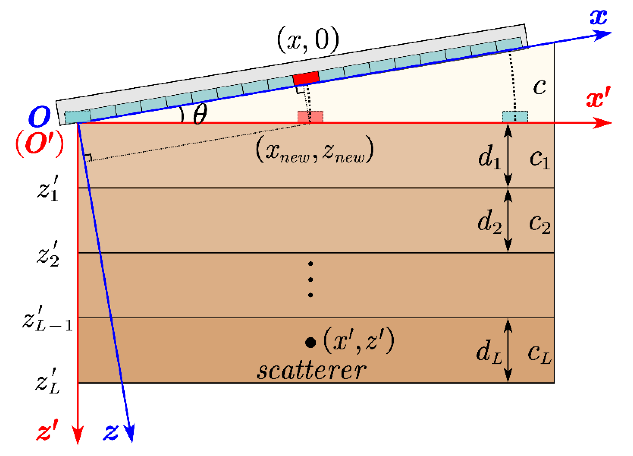
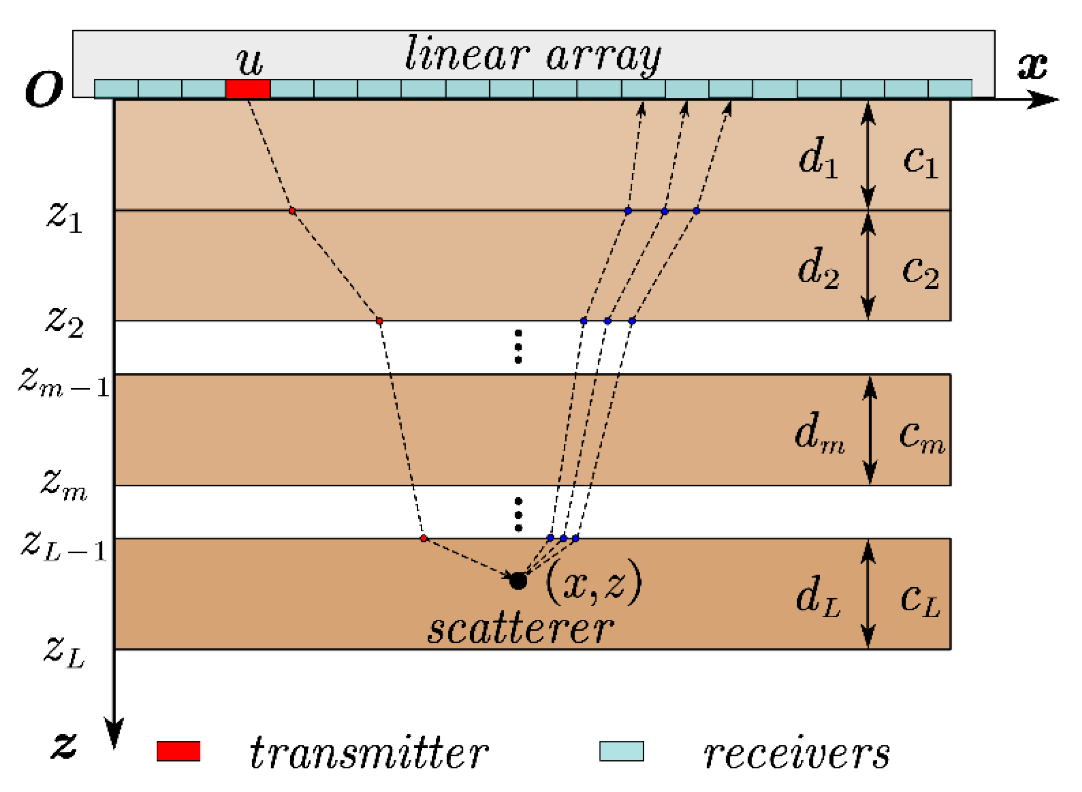
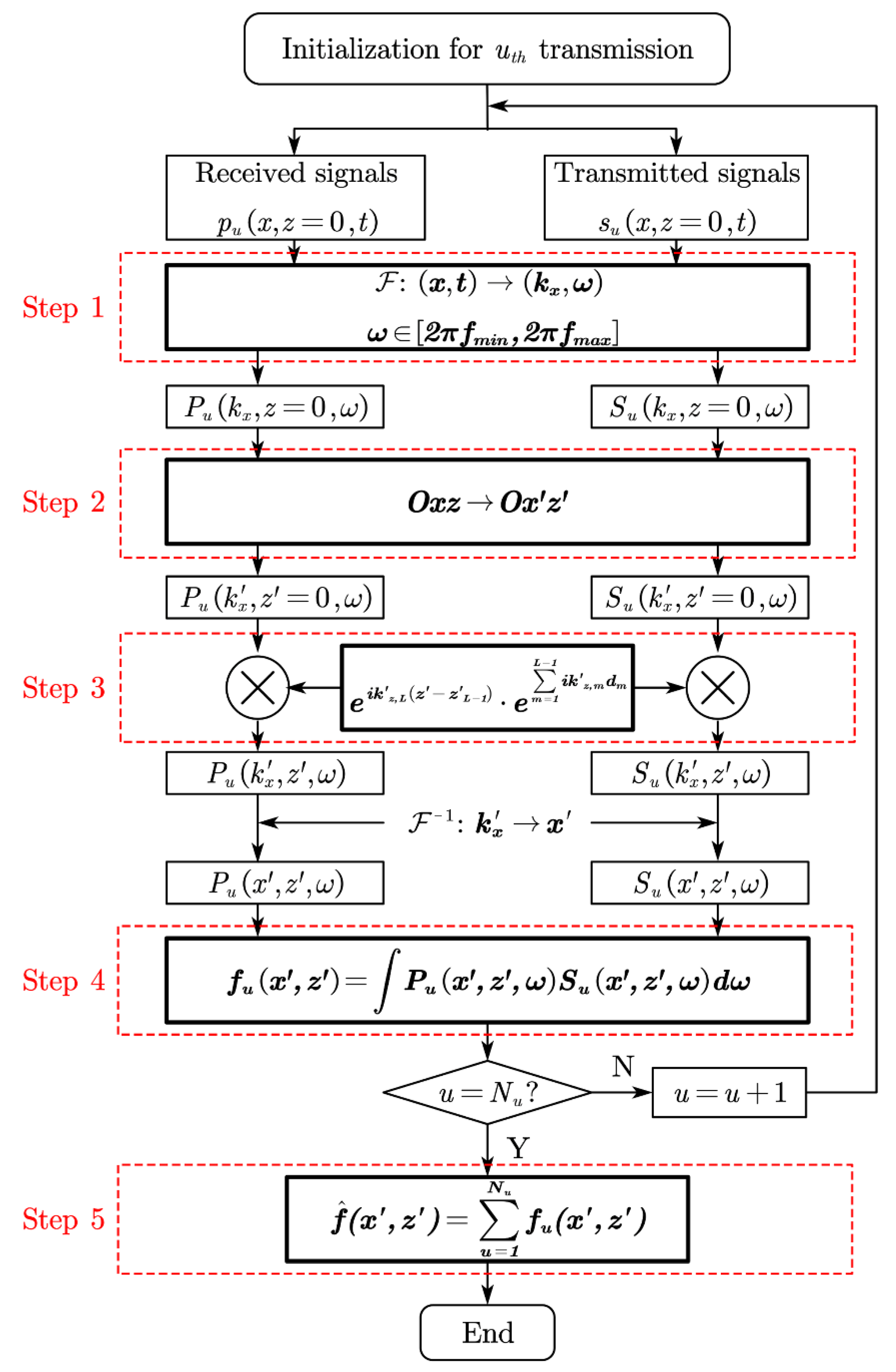
2.1. Wave-Field Extrapolation for Multi-Layered Structures
2.2. Oblique Incidence Compensation
2.3. Full-Matrix Imaging in Wavenumber Domain
2.4. Implementation
3. Results
3.1. Simulation
3.2. Experiments
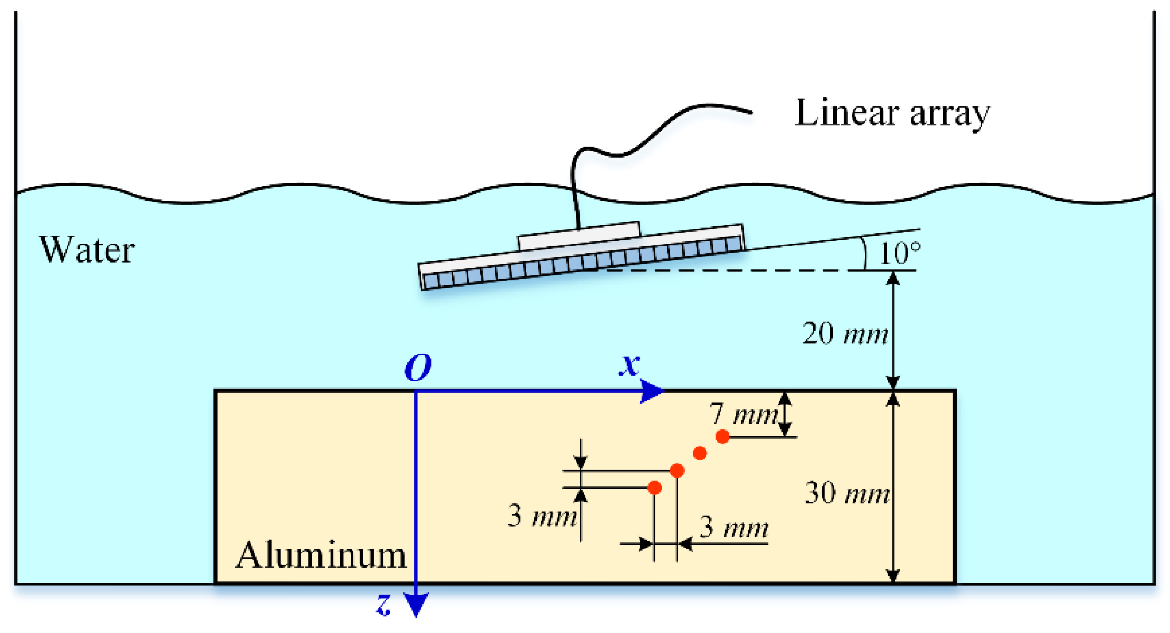
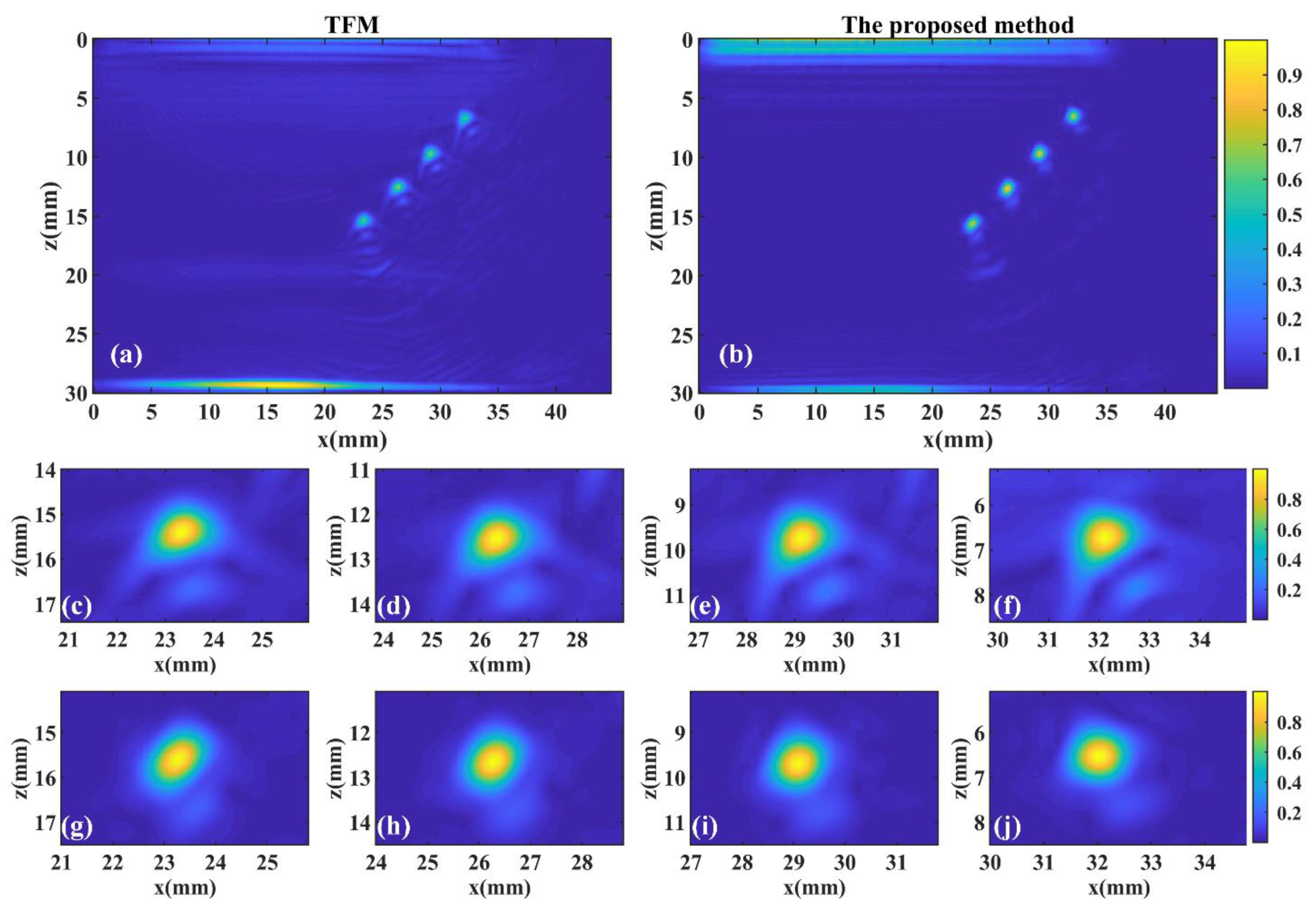
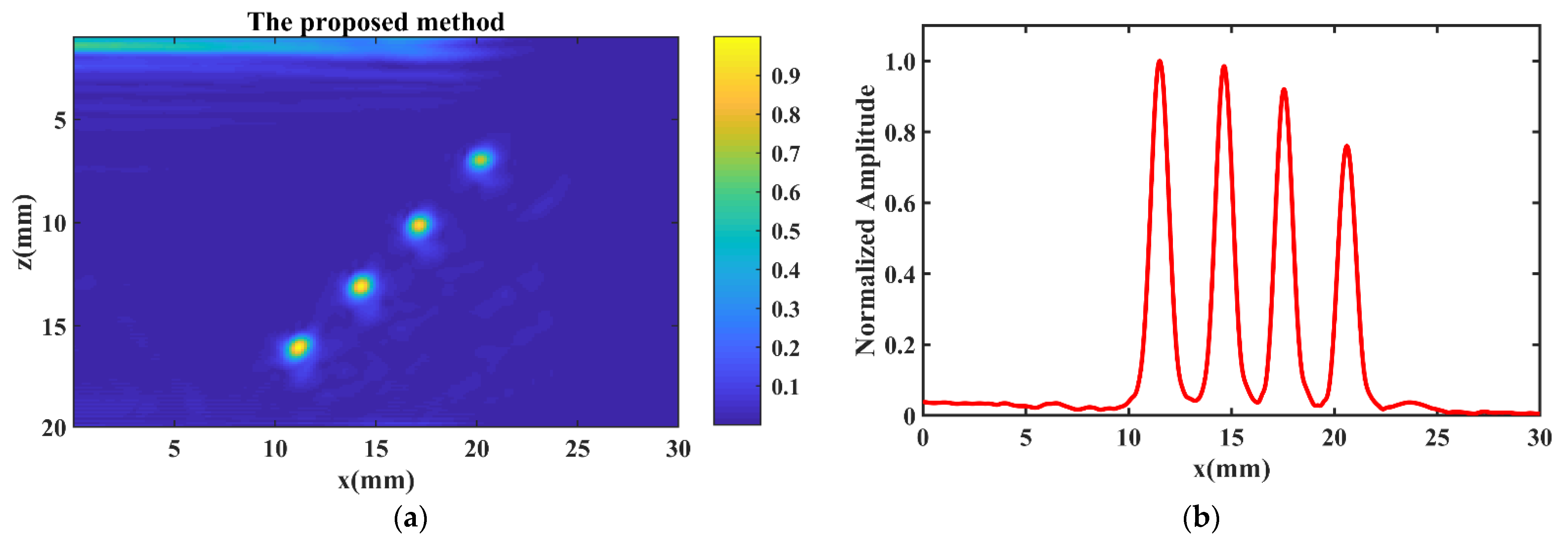
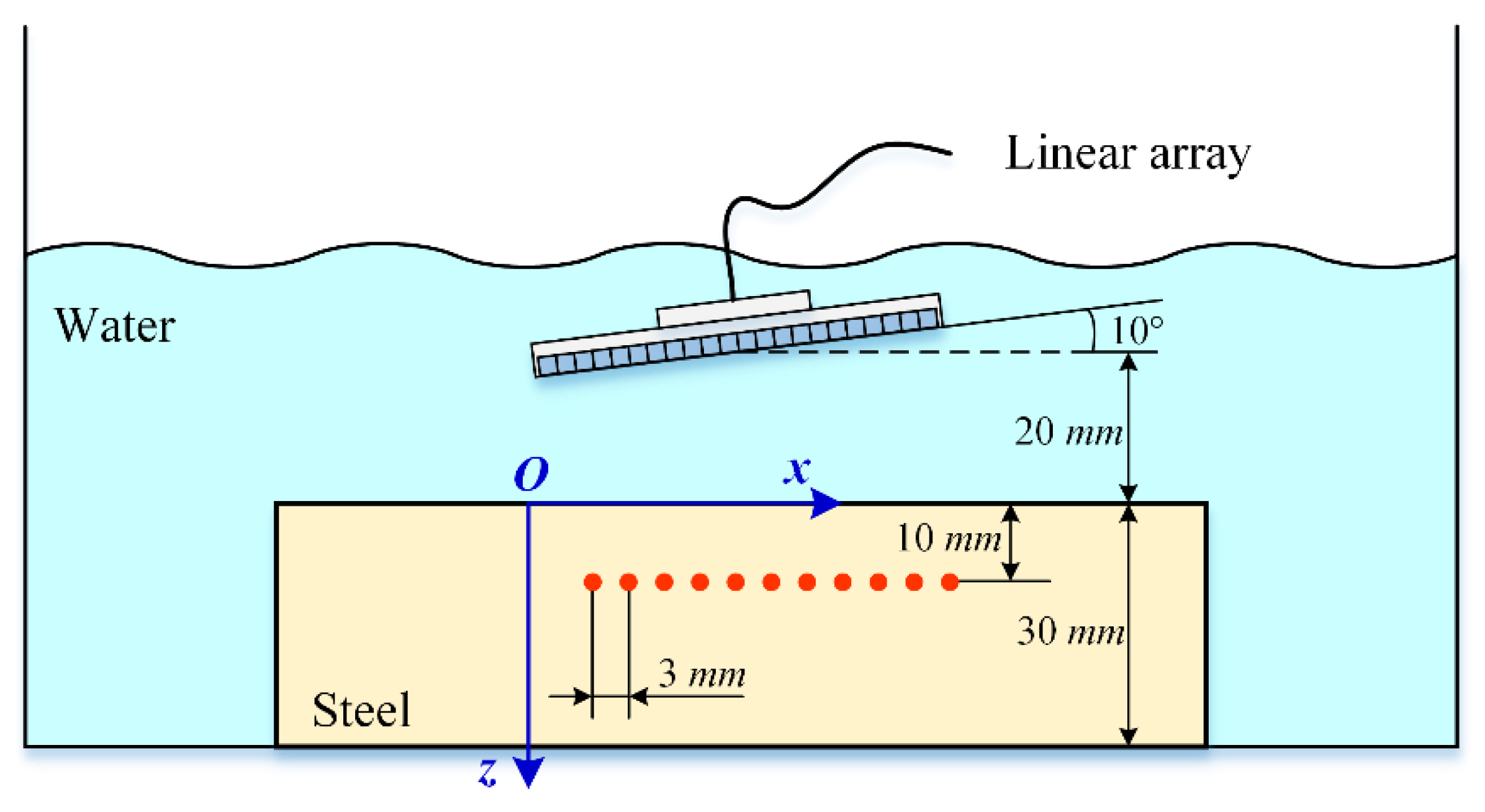
3.2.1. Experiment A
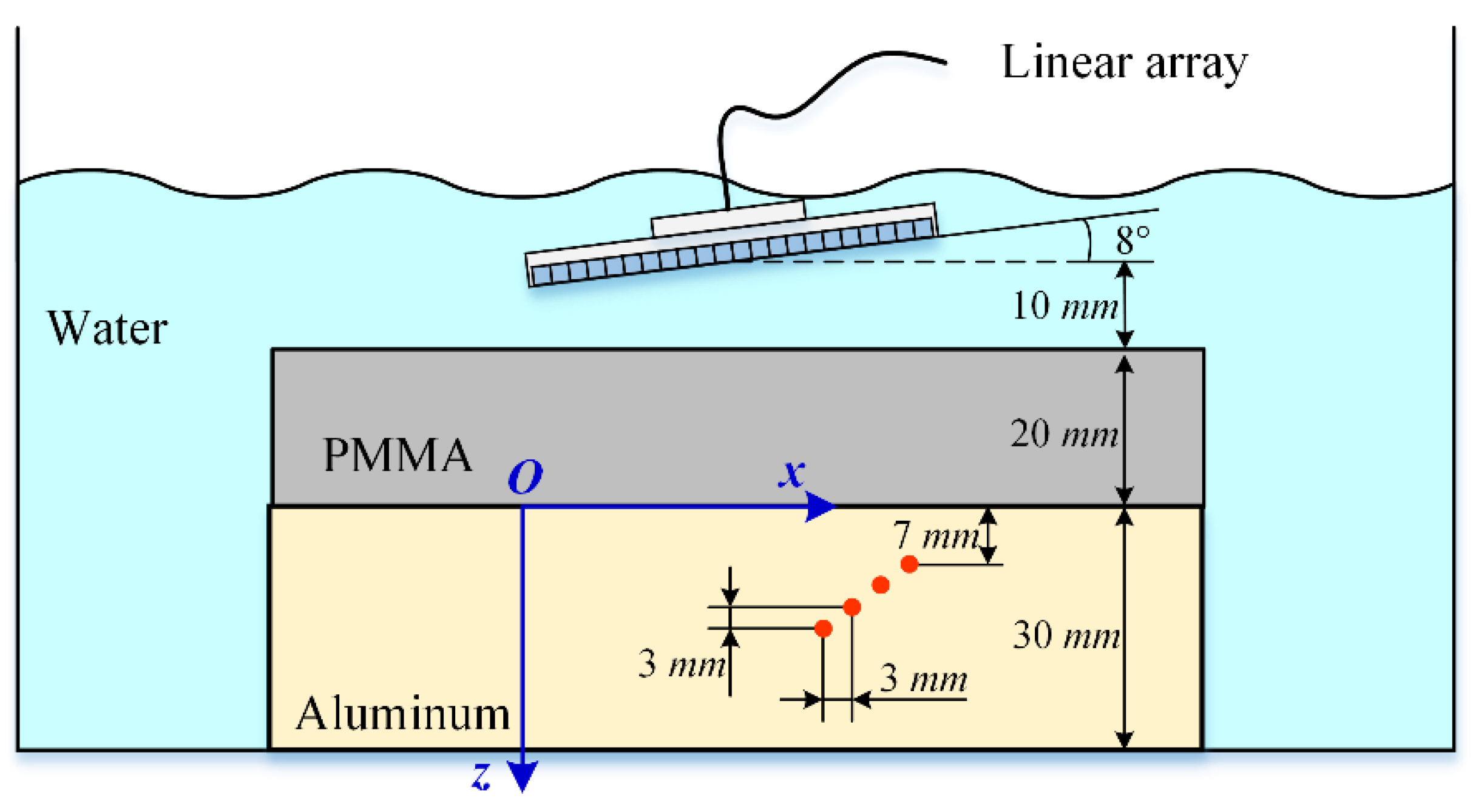
3.2.2. Experiment B
3.2.3. Experiment C
4. Discussion
5. Conclusions
Author Contributions
Funding
Institutional Review Board Statement
Informed Consent Statement
Data Availability Statement
Conflicts of Interest
References
- Felice, M.V.; Fan, Z. Sizing of flaws using ultrasonic bulk wave testing: A review. Ultrasonics 2018, 88, 26–42. [Google Scholar] [CrossRef] [PubMed]
- Honarvar, F.; Varvani-Farahani, A. A review of ultrasonic testing applications in additive manufacturing: Defect evaluation, material characterization, and process control. Ultrasonics 2020, 108, 106227. [Google Scholar] [CrossRef] [PubMed]
- Feng, L.; Qian, X. Enhanced sizing for surface cracks in welded tubular joints using ultrasonic phased array and image processing. NDT E Int. 2020, 116, 102334. [Google Scholar] [CrossRef]
- Drinkwater, B.W.; Wilcox, P.D. Ultrasonic arrays for non-destructive evaluation: A review. NDT E Int. 2006, 39, 525–541. [Google Scholar] [CrossRef]
- Malkin, R.E.; Franklin, A.C.; Bevan, R.L.T.; Kikura, H.; Drinkwater, B.W. Surface reconstruction accuracy using ultrasonic arrays: Application to non-destructive testing. NDT E Int. 2018, 96, 26–34. [Google Scholar] [CrossRef] [Green Version]
- Ménard, C.; Robert, S.; Miorelli, R.; Lesselier, D. Optimization algorithms for ultrasonic array imaging in homogeneous anisotropic steel components with unknown properties. NDT E Int. 2020, 116, 102327. [Google Scholar] [CrossRef]
- Dupont-Marillia, F.; Jahazi, M.; Lafreniere, S.; Belanger, P. Design and optimisation of a phased array transducer for ultrasonic inspection of large forged steel ingots. NDT E Int. 2019, 103, 119–129. [Google Scholar] [CrossRef]
- Li, W.; Zhou, Z.; Li, Y. Inspection of butt welds for complex surface parts using ultrasonic phased array. Ultrasonics 2019, 96, 75–82. [Google Scholar] [CrossRef]
- Ahmad, R.; Kundu, T.; Placko, D. Modeling of phased array transducers. J. Acoust. Soc. Am. 2005, 117, 1762–1776. [Google Scholar] [CrossRef]
- Raišutis, R.; Tumšys, O.; Kažys, R. Development of the technique for independent dual focusing of contact type ultrasonic phased array transducer in two orthogonal planes. NDT E Int. 2017, 88, 71–80. [Google Scholar] [CrossRef]
- Holmes, C.; Drinkwater, B.W.; Wilcox, P.D. Post-processing of the full matrix of ultrasonic transmit–receive array data for non-destructive evaluation. NDT E Int. 2005, 38, 701–711. [Google Scholar] [CrossRef]
- Potter, J.N.; Wilcox, P.D.; Croxford, A.J. Diffuse field full matrix capture for near surface ultrasonic imaging. Ultrasonics 2018, 82, 44–48. [Google Scholar] [CrossRef] [Green Version]
- Zhang, J.; Drinkwater, B.W.; Wilcox, P.D.; Hunter, A.J. Defect detection using ultrasonic arrays: The multi-mode total focusing method. NDT E Int. 2010, 43, 123–133. [Google Scholar] [CrossRef]
- Lin, L.; Cao, H.; Luo, Z. Total focusing method imaging of multidirectional CFRP laminate with model-based time delay correction. NDT E Int. 2018, 97, 51–58. [Google Scholar] [CrossRef]
- Fan, C.; Caleap, M.; Pan, M.; Drinkwater, B.W. A comparison between ultrasonic array beamforming and super resolution imaging algorithms for non-destructive evaluation. Ultrasonics 2014, 54, 1842–1850. [Google Scholar] [CrossRef] [Green Version]
- Hunter, A.J.; Drinkwater, B.W.; Wilcox, P.D. The wavenumber algorithm for full-matrix imaging using an ultrasonic array. IEEE Trans. Ultrason. Ferroelectr. Freq. Control 2008, 55, 2450–2462. [Google Scholar] [CrossRef]
- Wu, H.; Chen, J.; Yang, K.; Hu, X. Ultrasonic array imaging of multilayer structures using full matrix capture and extended phase shift migration. Meas. Sci. Technol. 2016, 27, 045401. [Google Scholar] [CrossRef]
- Jin, H.; Chen, J. An efficient wavenumber algorithm towards real-time ultrasonic full-matrix imaging of multi-layered medium. Mech. Syst. Signal Process. 2021, 149, 107149. [Google Scholar] [CrossRef]
- Skjelvareid, M.H.; Olofsson, T.; Birkelund, Y.; Larsen, Y. Synthetic aperture focusing of ultrasonic data from multilayered media using an omega-k algorithm. IEEE Trans. Ultrason. Ferroelectr. Freq. Control 2011, 58, 1037–1048. [Google Scholar] [CrossRef] [Green Version]
- Lhémery, A.; Calmon, P.; Lecœur-Taıbi, I.; Raillon, R.; Paradis, L. Modeling tools for ultrasonic inspection of welds. NDT E Int. 2000, 33, 499–513. [Google Scholar] [CrossRef]
- Wang, X.X.; He, C.; Zhao, P.Z.; Zheng, Y.; Jiang, S.H.; Wei, Y.D. Non-Destructive Detection of GIS Aluminum Alloy Shell Weld Based on Oblique Incidence Full Focus Method. In Materials Science Forum; Trans Tech Publications Ltd.: Bäch, Switzerland, 2020; Volume 1007, pp. 105–110. [Google Scholar] [CrossRef]
- Cao, H.; Guo, S.; Zhang, S.; Xie, Y.; Feng, W. Ray tracing method for ultrasonic array imaging of CFRP corner part using homogenization method. NDT E Int. 2021, 122, 102493. [Google Scholar] [CrossRef]
- Kolkoori, S.; Hoehne, C.; Prager, J.; Rethmeier, M.; Kreutzbruck, M. Quantitative evaluation of ultrasonic C-scan image in acoustically homogeneous and layered anisotropic materials using three dimensional ray tracing method. Ultrasonics 2014, 54, 551–562. [Google Scholar] [CrossRef] [PubMed]
- Haunt, M.A.; Jones, D.L.; Brien, W.D.O. Adaptive focusing through layered media using the geophysical “time migration” concept. In Proceedings of the 2002 IEEE Ultrasonics Symposium, Munich, Germany, 8–11 October 2002; Volume 1632, pp. 1635–1638. [Google Scholar] [CrossRef]
- Skjelvareid, M.H.; Birkelund, Y. Ultrasound Imaging Using Multilayer Synthetic Aperture Focusing. In Proceedings of the ASME 2010 Pressure Vessels and Piping Division/K-PVP Conference, Washington, DC, USA, 18–22 July 2010; pp. 379–387. [Google Scholar] [CrossRef]
- Cruza, J.F.; Camacho, J. Total Focusing Method with Virtual Sources in the Presence of Unknown Geometry Interfaces. IEEE Trans. Ultrason. Ferroelectr. Freq. Control 2016, 63, 1581–1592. [Google Scholar] [CrossRef] [PubMed]
- Kumar, A. Phased array ultrasonic imaging using angle beam virtual source full matrix capture-total focusing method. NDT E Int. 2020, 116, 102324. [Google Scholar] [CrossRef]
- Lukomski, T. Full-matrix capture with phased shift migration for flaw detection in layered objects with complex geometry. Ultrasonics 2016, 70, 241–247. [Google Scholar] [CrossRef]
- Leonid, M.; Brekhovskikh, O.A.G. Acoustics of Layered Media I (Springer Series on Wave Phenomena, no. 0931-7252); Springer Science & Business Media: Berlin/Heidelberg, Germany, 1990. [Google Scholar] [CrossRef]
- Olofsson, T. Phase shift migration for imaging layered objects and objects immersed in water. IEEE Trans. Ultrason. Ferroelectr. Freq. Control 2010, 57, 2522–2530. [Google Scholar] [CrossRef] [Green Version]
- Montaldo, G.; Tanter, M.; Bercoff, J.; Benech, N.; Fink, M. Coherent plane-wave compounding for very high frame rate ultrasonography and transient elastography. IEEE Trans. Ultrason. Ferroelectr. Freq. Control 2009, 56, 489–506. [Google Scholar] [CrossRef]


| Array Parameter | Value |
|---|---|
| Number of elements | 64 |
| Element pitch | 0.6 mm |
| Element width | 0.6 mm |
| Element length | 10 mm |
| Center frequency | 5 MHz |
| −6 dB bandwidth | 78% |
| Methods | SDH 2 | SDH 4 | SDH 6 | SDH 8 | SDH 10 | Average | Time Cost | ||||||
|---|---|---|---|---|---|---|---|---|---|---|---|---|---|
| API | FWHM | API | FWHM | API | FWHM | API | FWHM | API | FWHM | API | FWHM | ||
| Time-domain TFM | 0.7068 | 0.9937 | 0.7013 | 1.0313 | 0.7233 | 1.05 | 0.7356 | 1.0125 | 0.7648 | 1.0125 | 0.7264 | 1.02 | 258.12 s |
| Proposed method | 0.7666 | 1.0813 | 0.6853 | 1.0125 | 0.6670 | 0.9 | 0.6756 | 0.9188 | 0.7431 | 0.9562 | 0.7070 | 0.9738 | 4.31 s |
| Difference | +8.5% | +8.8% | −2.3% | −1.8% | −7.8% | −14.3% | −8.2% | −9.3% | −2.8% | −5.6% | −2.3% | −4.5% | −98.3% |
| Parameter | Value |
|---|---|
| Pulse width | 100 ns |
| Pulse voltage | −100 V |
| Sampling frequency | 50 MHz |
| Sample points | 4096 |
| Amplifier gain | 30 dB |
| Digitization | 14 bit |
| Methods | SDH 1 | SDH 2 | SDH 3 | SDH 4 | Average | Time Cost | |||||
|---|---|---|---|---|---|---|---|---|---|---|---|
| API | FWHM | API | FWHM | API | FWHM | API | FWHM | API | FWHM | ||
| Time-domain TFM | 0.7640 | 1.0125 | 0.7374 | 1.0125 | 0.7204 | 1.0323 | 0.6993 | 1.0687 | 0.7302 | 1.0315 | 255.89 s |
| Proposed method | 0.6473 | 0.9652 | 0.6503 | 0.9375 | 0.6834 | 0.9750 | 0.6956 | 1.0125 | 0.6691 | 0.9726 | 4.25 s |
| Difference | −15.3% | −4.8% | −11.2% | −7.4% | −5.1% | −5.6% | −0.5% | −5.3% | −8.4% | −5.7% | −98.3% |
| Items | FWHM: SDH1 | FWHM: SDH2 | FWHM: SDH3 | FWHM: SDH4 | Average FWHM | SNR | Time Cost |
|---|---|---|---|---|---|---|---|
| Values | 1.038 mm | 0.999 mm | 0.987 mm | 1.023 mm | 1.012 mm | 26.18 | 3.02 s |
Publisher’s Note: MDPI stays neutral with regard to jurisdictional claims in published maps and institutional affiliations. |
© 2021 by the authors. Licensee MDPI, Basel, Switzerland. This article is an open access article distributed under the terms and conditions of the Creative Commons Attribution (CC BY) license (https://creativecommons.org/licenses/by/4.0/).
Share and Cite
Yu, B.; Jin, H.; Mei, Y.; Chen, J.; Wu, E.; Yang, K. A Modified Wavenumber Algorithm of Multi-Layered Structures with Oblique Incidence Based on Full-Matrix Capture. Appl. Sci. 2021, 11, 10808. https://doi.org/10.3390/app112210808
Yu B, Jin H, Mei Y, Chen J, Wu E, Yang K. A Modified Wavenumber Algorithm of Multi-Layered Structures with Oblique Incidence Based on Full-Matrix Capture. Applied Sciences. 2021; 11(22):10808. https://doi.org/10.3390/app112210808
Chicago/Turabian StyleYu, Bei, Haoran Jin, Yujian Mei, Jian Chen, Eryong Wu, and Keji Yang. 2021. "A Modified Wavenumber Algorithm of Multi-Layered Structures with Oblique Incidence Based on Full-Matrix Capture" Applied Sciences 11, no. 22: 10808. https://doi.org/10.3390/app112210808
APA StyleYu, B., Jin, H., Mei, Y., Chen, J., Wu, E., & Yang, K. (2021). A Modified Wavenumber Algorithm of Multi-Layered Structures with Oblique Incidence Based on Full-Matrix Capture. Applied Sciences, 11(22), 10808. https://doi.org/10.3390/app112210808