
Memory Model for Morphological Semantics of Visual Stimuli Using Sparse Distributed Representation


Abstract
Featured Application
Abstract
1. Introduction
2. Related Researches
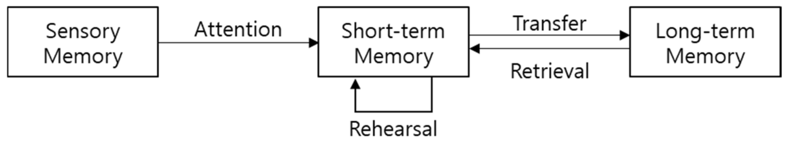
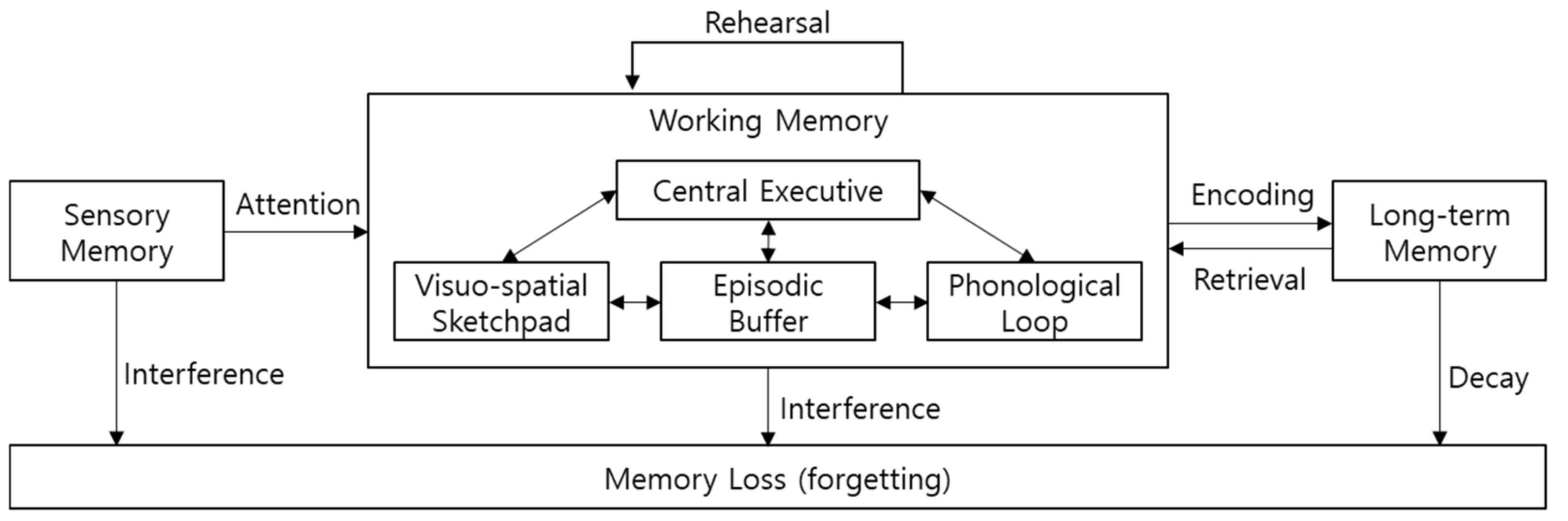
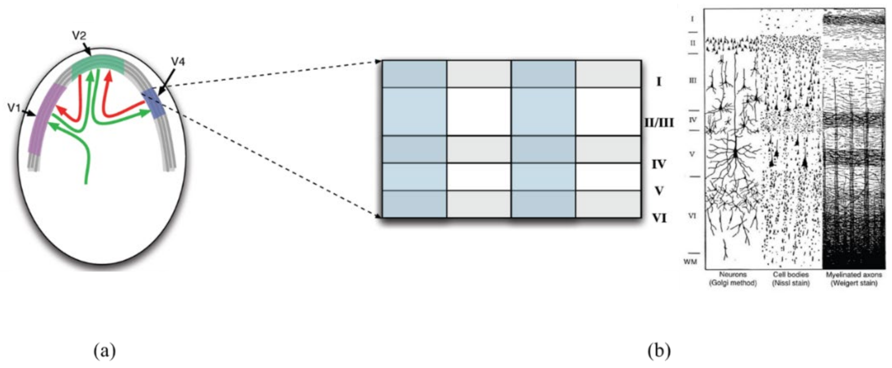
2.1. Cognitive Psychological Memory Researches
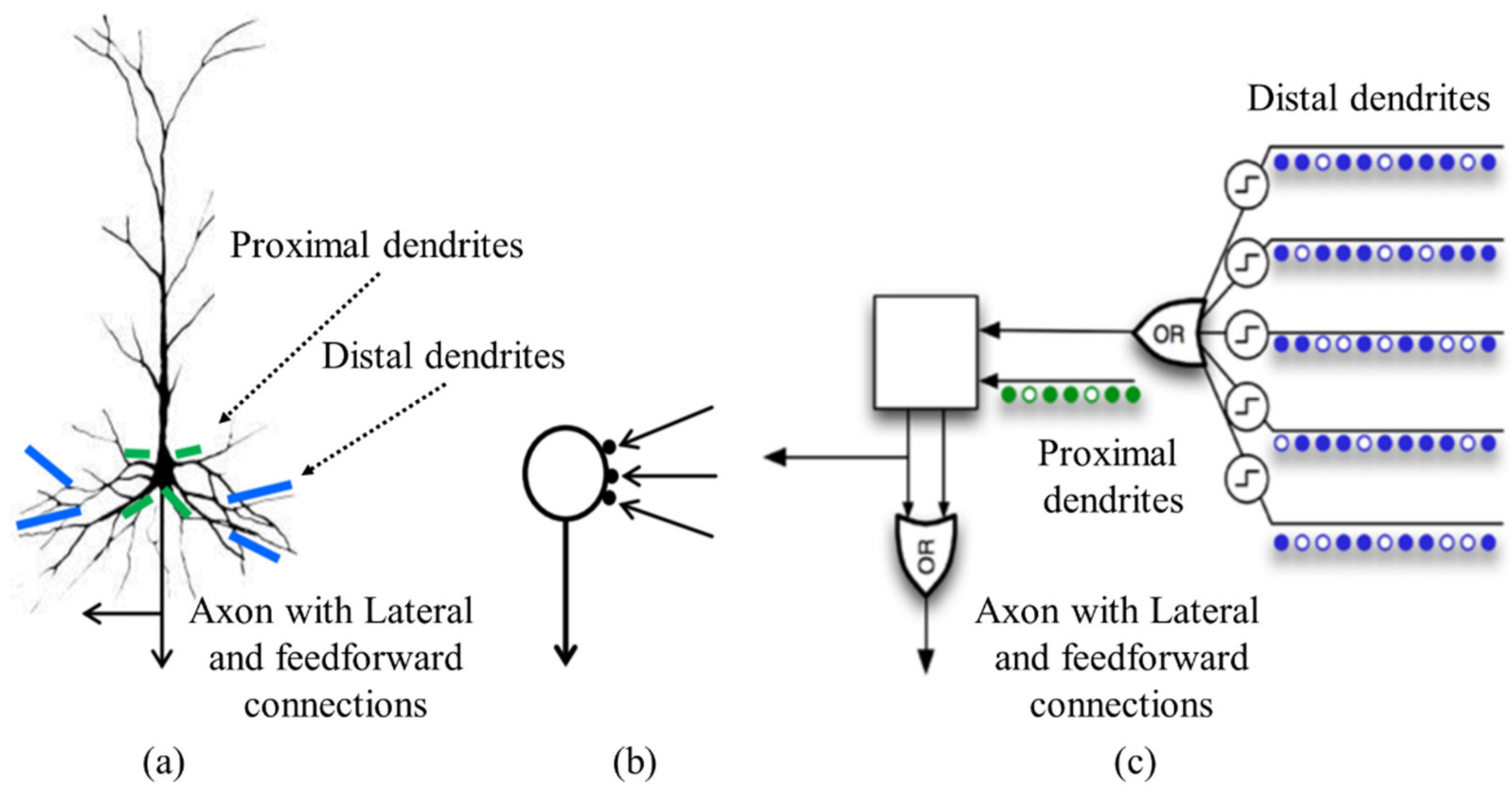
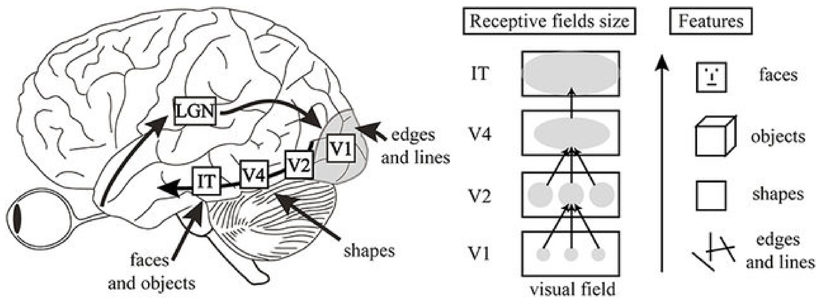
2.2. Computing Models for Memory Mechanism
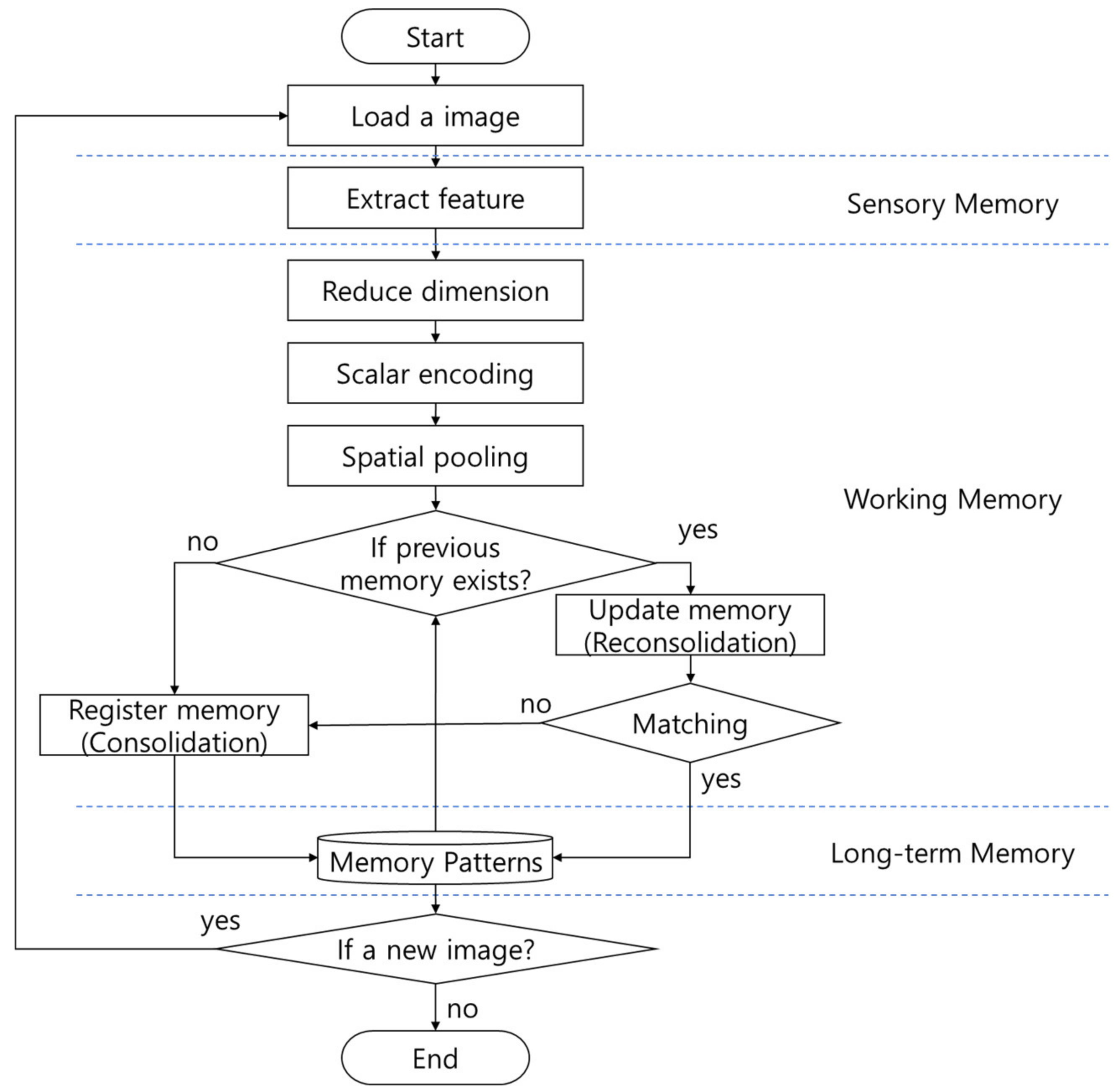
3. Morphological Semantics Memory Model for Visual Stimuli
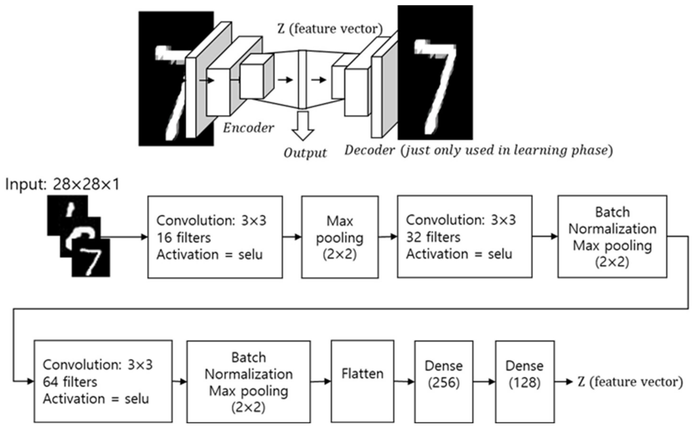
3.1. Sensory Memory: Feature Extraction by CNN-Autoencoder
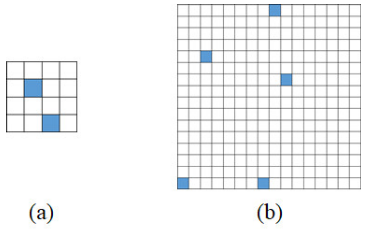
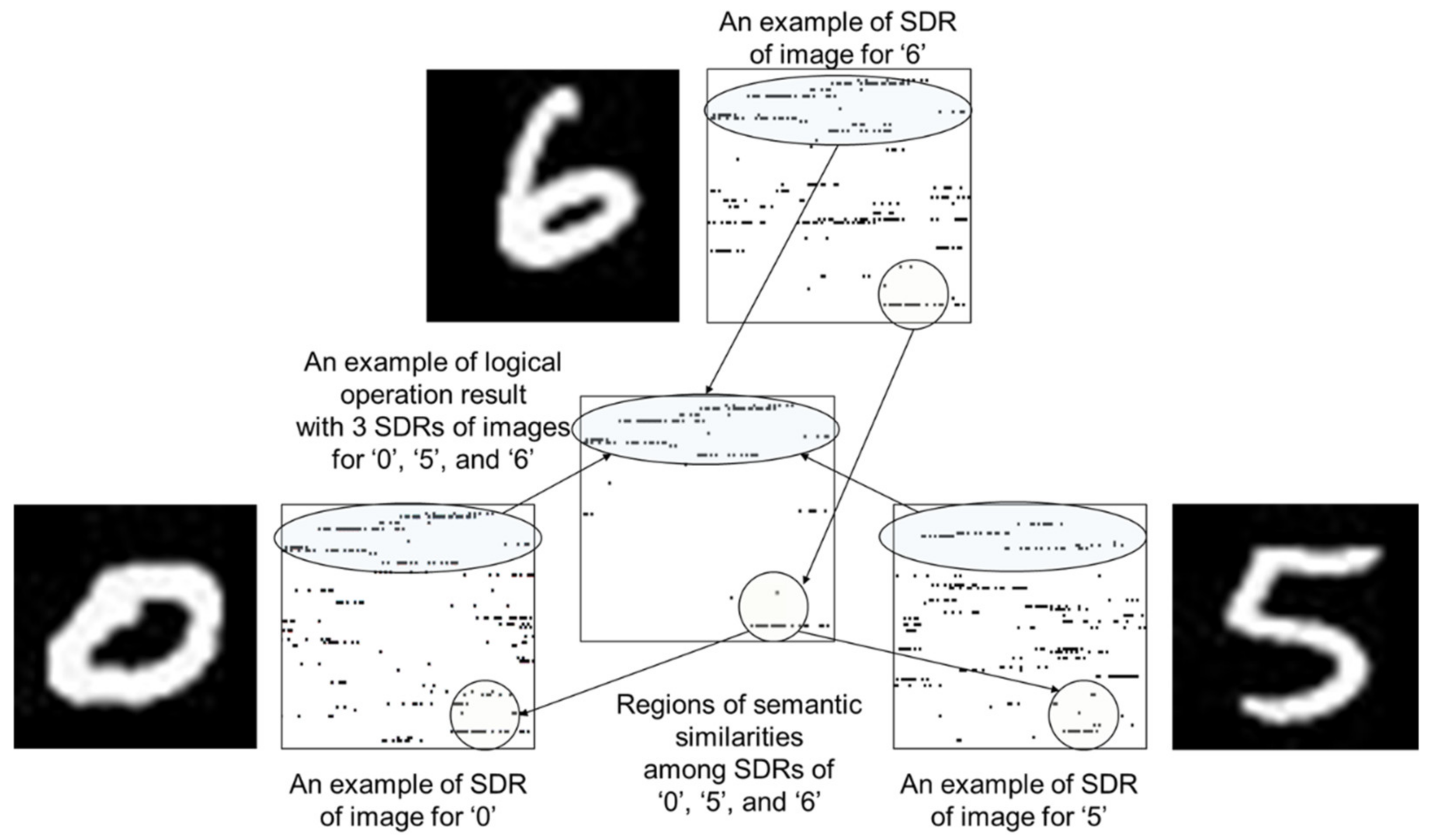
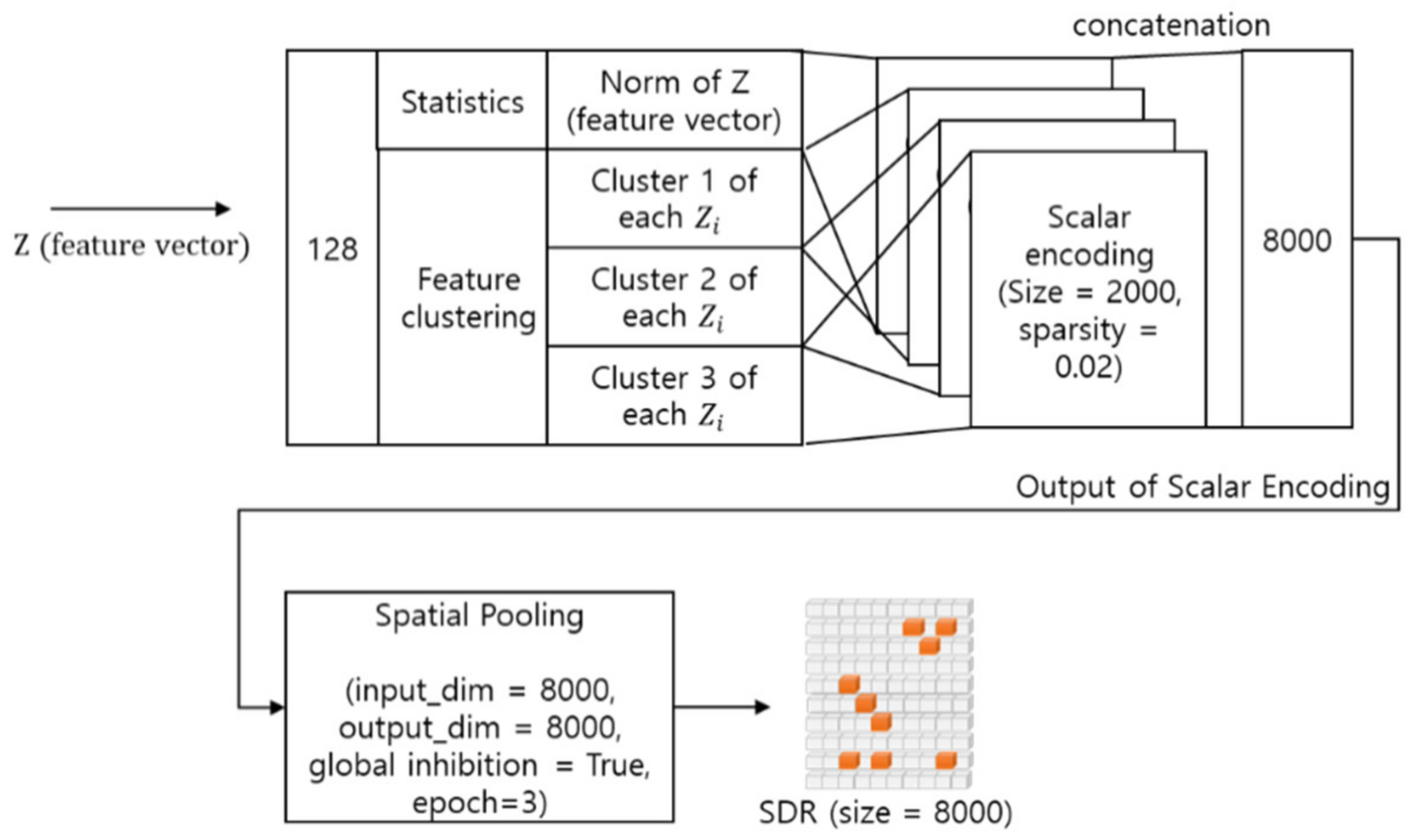
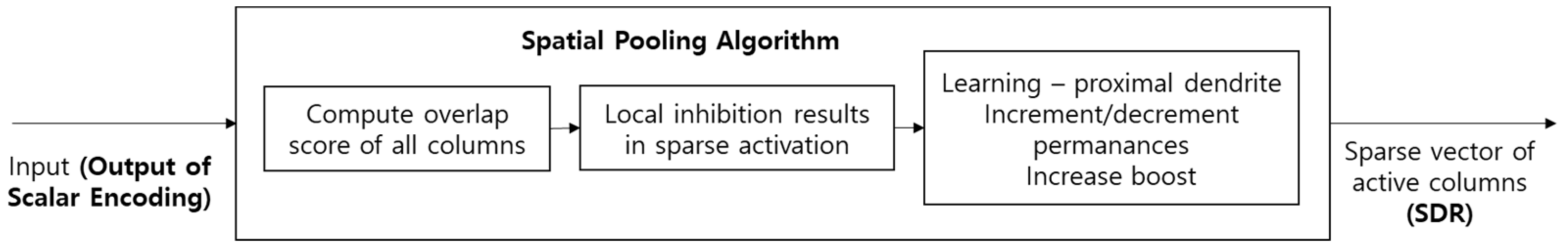
3.2. Working Memory: SDR Representation by Scalar Encoding and Spatial Pooling
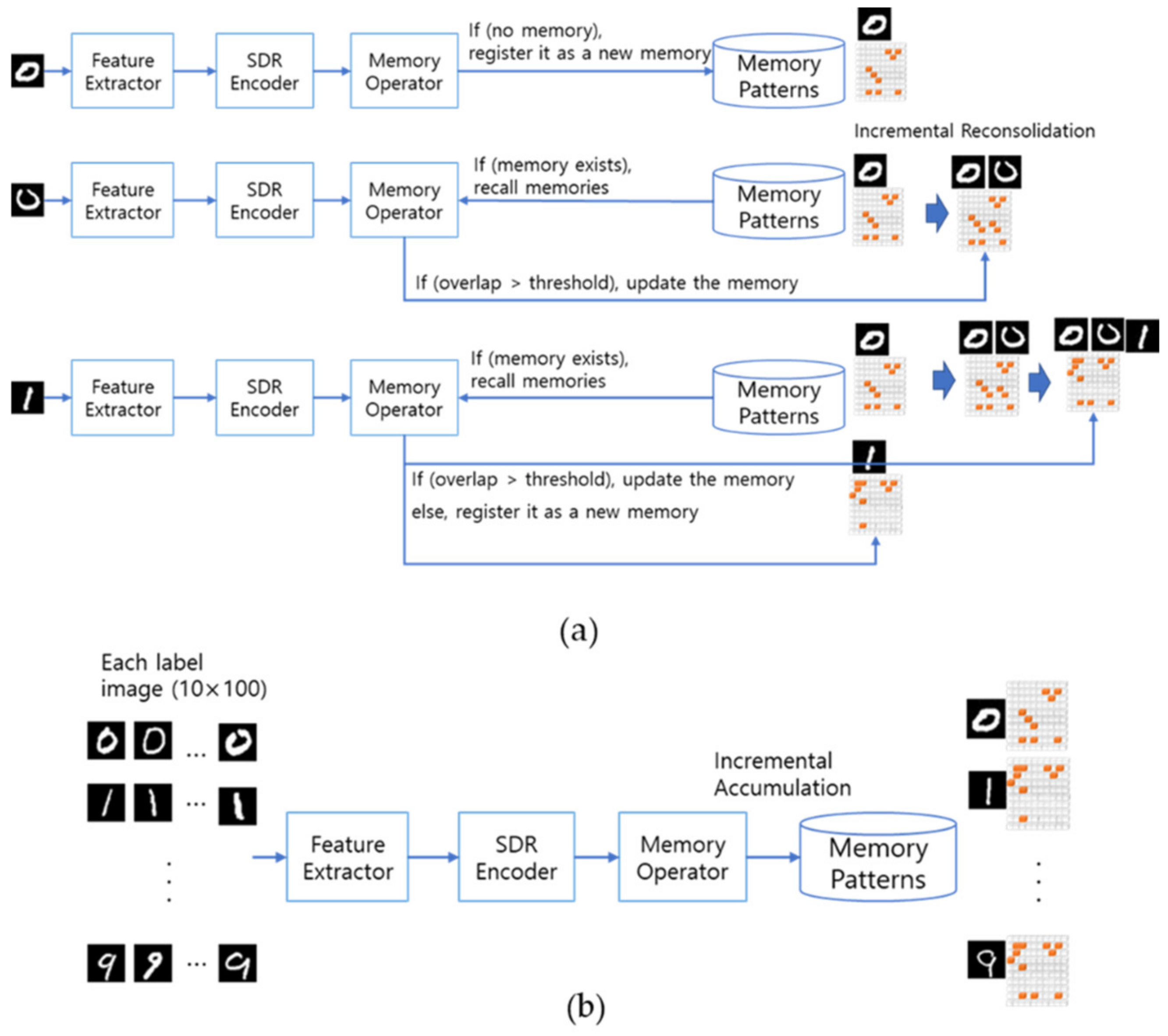
3.3. Working Memory: Memory Operation by Consolidation and Reconsolidation
3.4. Long-Term Memory: Memory Definition
4. Experimental Results
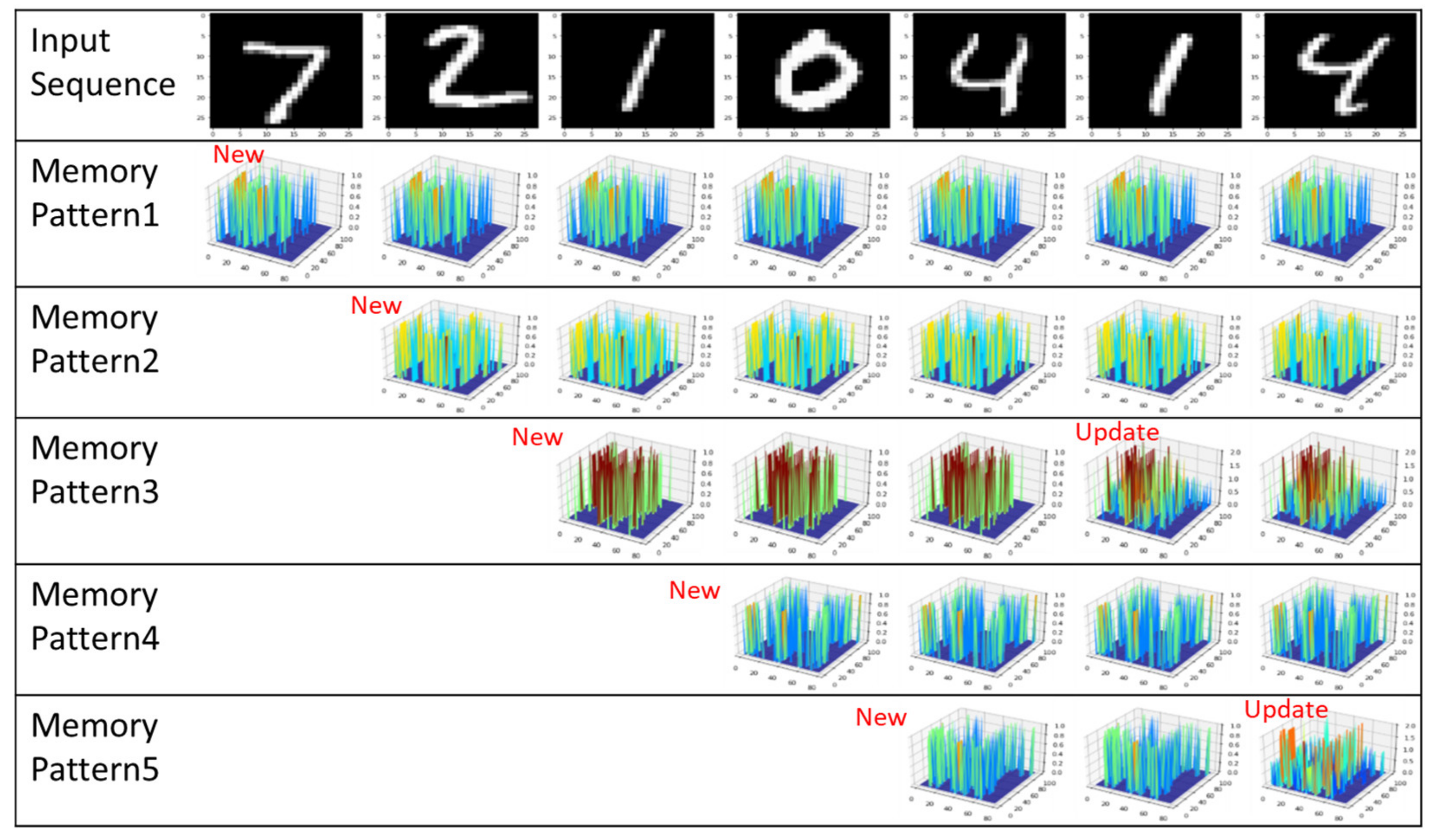
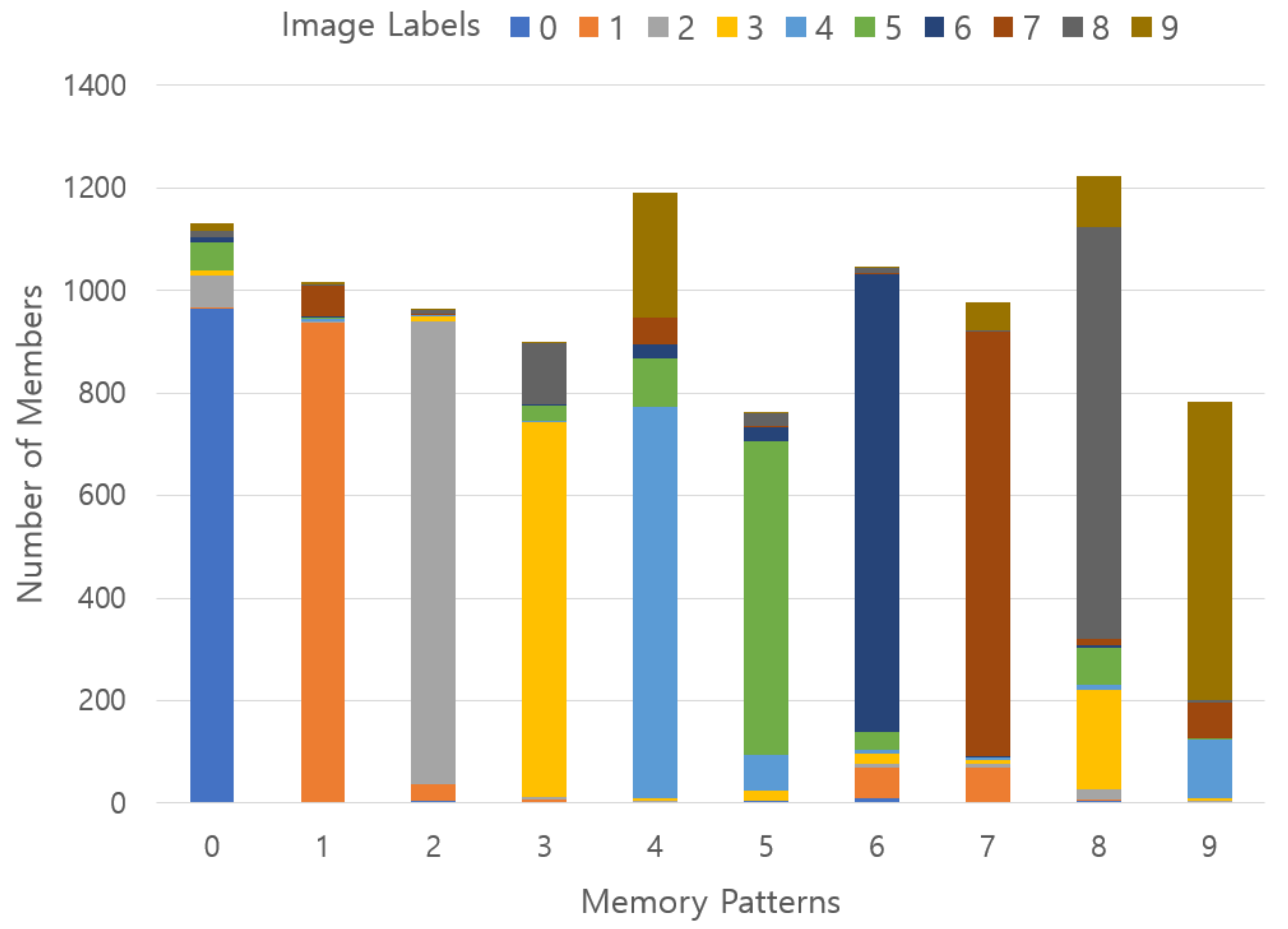
4.1. Experiment 1: Memory Pattern Formation Experiment without Pre-Memory Process
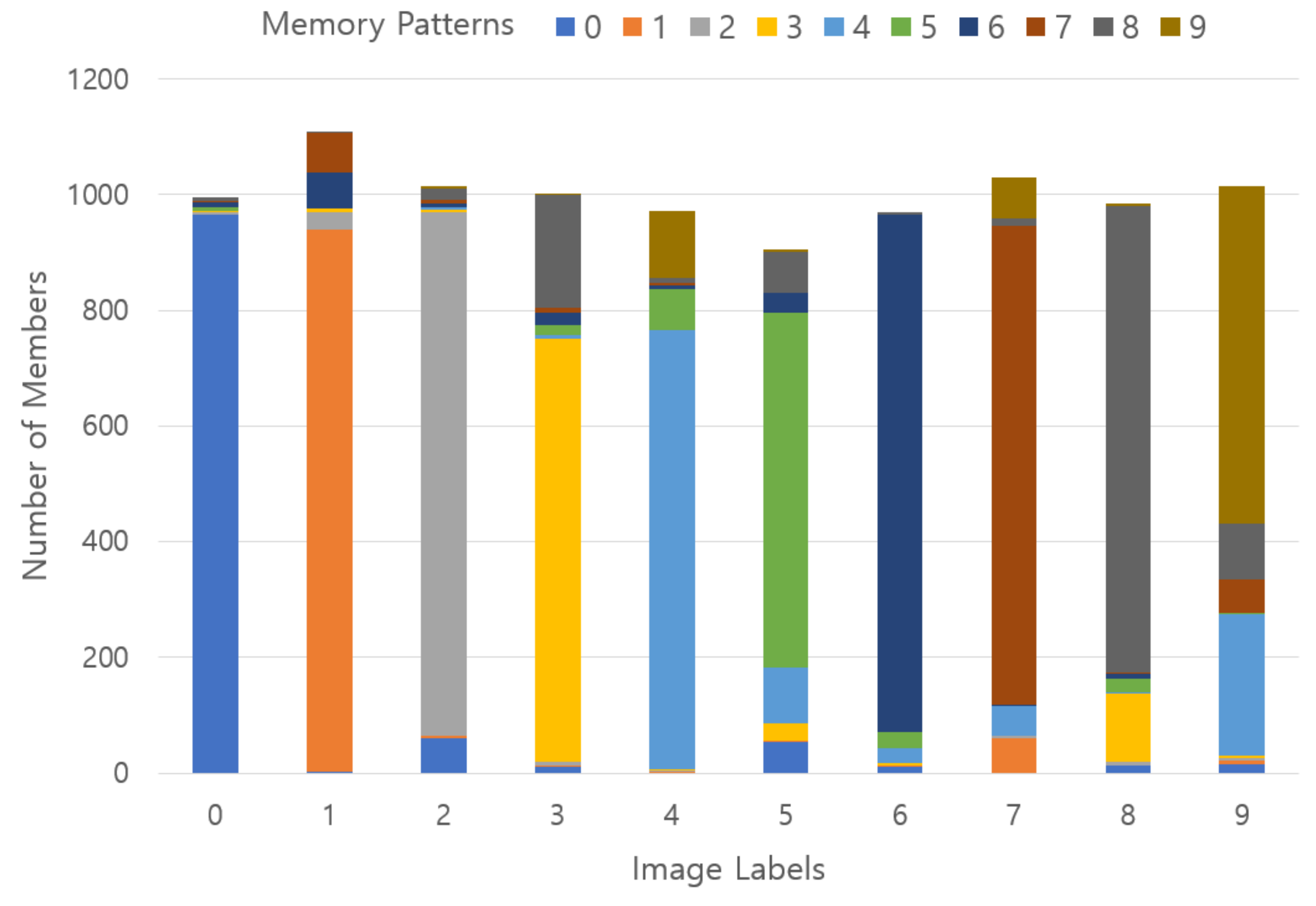
4.2. Experiment 2: Memory Pattern Formation Experiment Using Pre-Memory Process
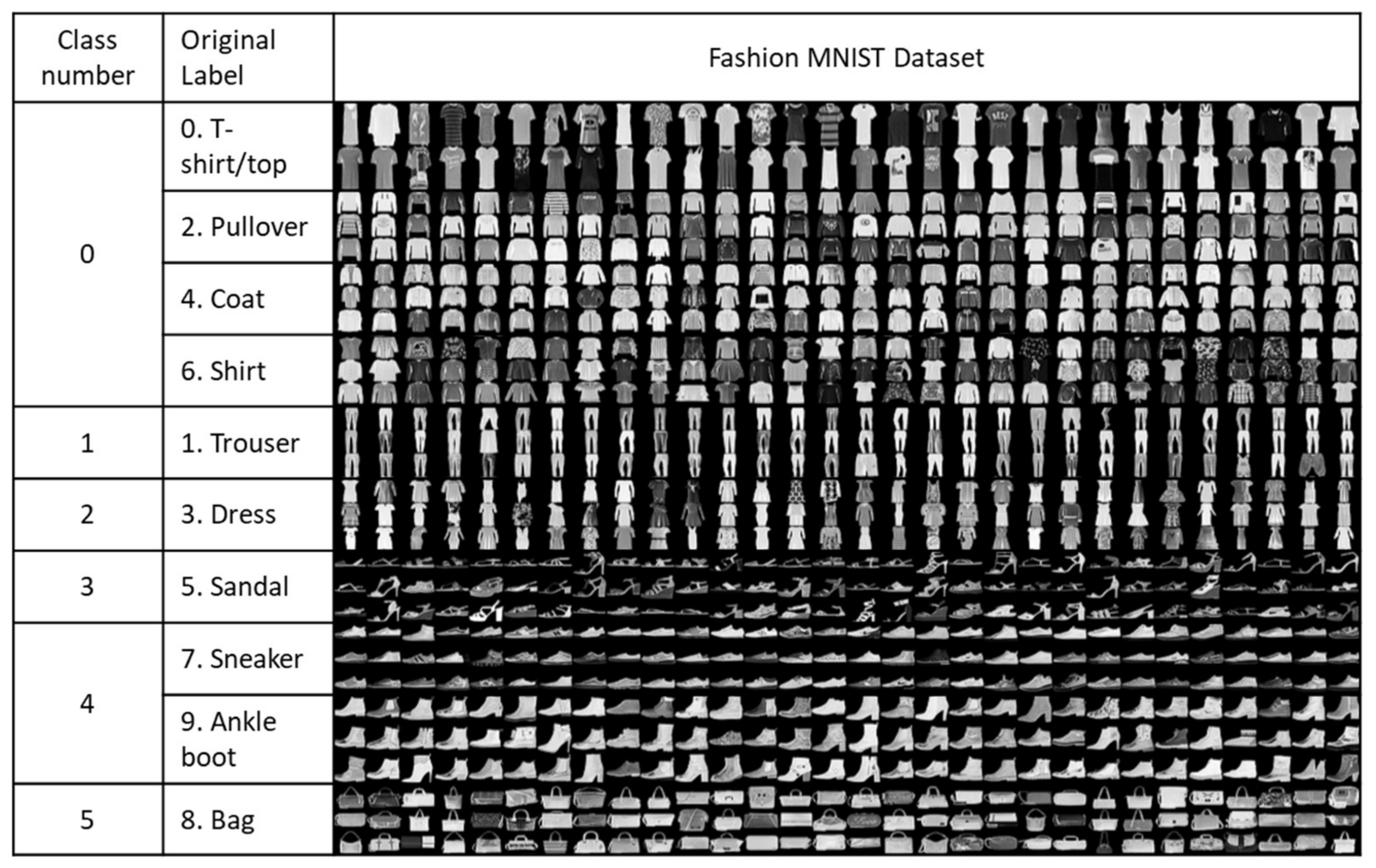
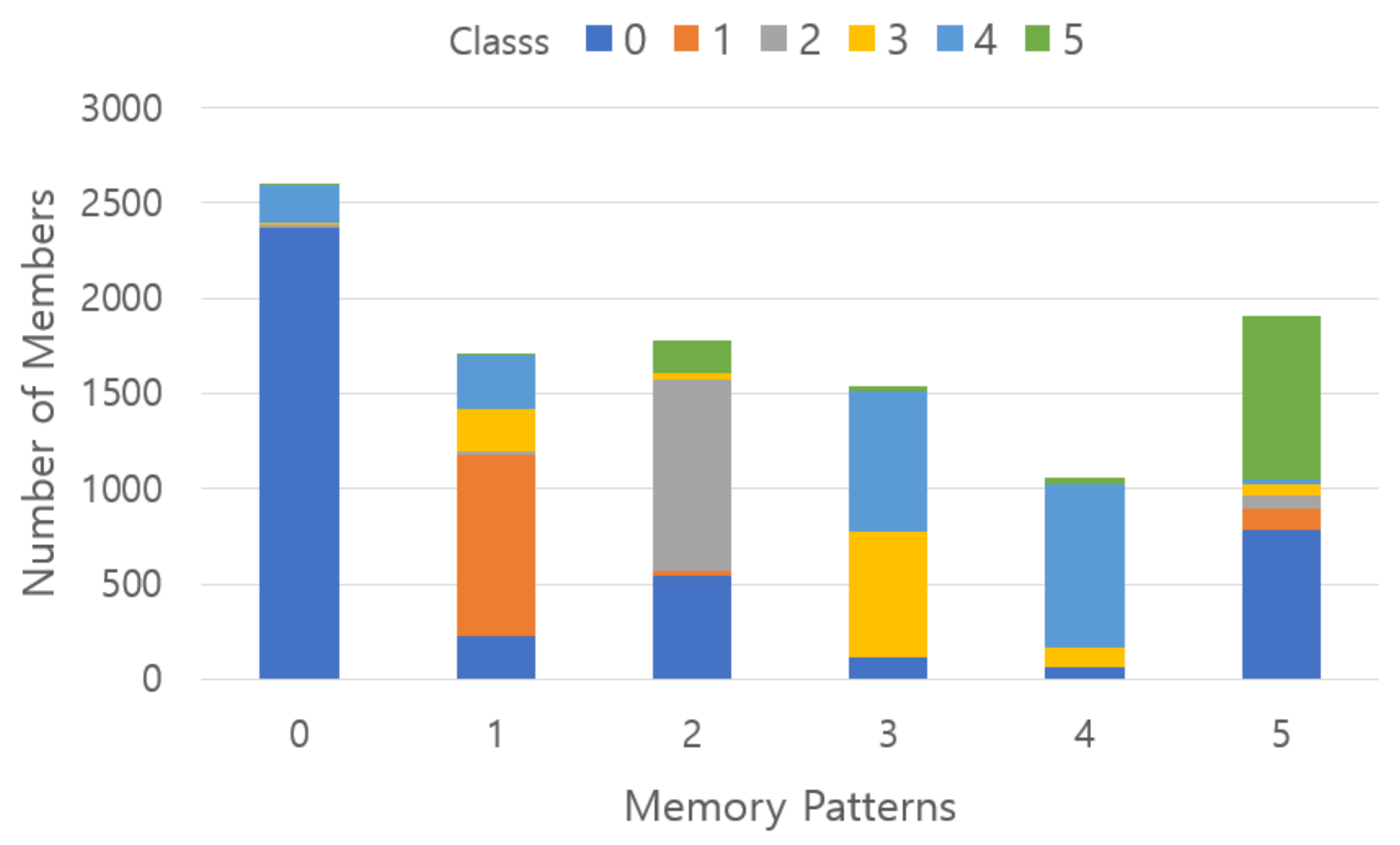
4.3. Experiment 3: Memory Pattern Formation Experiment Using Pre-Memory Process for Fashion-MNIST Dataset
4.4. Discussions
5. Conclusions
Author Contributions
Funding
Conflicts of Interest
References
- Hinton, G.E.; Osindero, S.; Teh, Y.-W. A Fast Learning Algorithm for Deep Belief Nets. Neural Comput. 2006, 18, 1527–1554. [Google Scholar] [CrossRef] [PubMed]
- LeCun, Y.; Bengio, Y.; Hinton, G. Deep learning. Nature 2015, 521, 436–444. [Google Scholar] [CrossRef] [PubMed]
- Goodfellow, I.; Pouget-Abadie, J.; Mirza, M.; Xu, B.; Warde-Farley, D.; Ozair, S.; Courville, A.; Bengio, Y. Generative adversarial nets. Adv. Neural Inf. Process. Syst. 2014, 27, 2672–2680. [Google Scholar]
- Eliasmith, C. How to Build a Brain: A Neural Architecture for Biological Cognition; Oxford Series on Cognitive Models and Architectures; Oxford University Press: Oxford, UK, 2013. [Google Scholar]
- Ahmad, S.; George, D.; Edwards, J.L.; Saphir, W.C.; Astier, F.; Marianetti, R. Hierarchical Temporal Memory (HTM) System Deployed as Web Service. U.S. Patent US20170180515A1, 20 May 2014. [Google Scholar]
- Hawkins, J.; Blakeslee, S. On Intelligence: How a New Understanding of the Brain Will Lead to the Creation of Truly Intelligent Machines; St. Martin’s Griffin, Macmillan: New York, NY, USA, 2007. [Google Scholar]
- Deng, L. The MNIST Database of Handwritten Digit Images for Machine Learning Research. IEEE Signal Process. Mag. 2012, 29, 141–142. [Google Scholar] [CrossRef]
- Xiao, H.; Rasul, K.; Vollgraf, R. Fashion-MNIST: A Novel Image Dataset for Benchmarking Machine Learning Algorithms. arXiv 2017, arXiv:1708.07747. [Google Scholar]
- Ebbinghaus, H. Memory: A Contribution to Experimental Psychology. Ann. Neurosci. 2013, 20, 155–156. [Google Scholar] [CrossRef] [PubMed]
- Bartlett, F.C.; Burt, C. Remembering: A Study in Experimental and Social Psychology; Cambridge University Press: Cambridge, UK, 1932. [Google Scholar]
- Atkinson, R.C.; Shiffrin, R.M. Chapter: Human memory: A proposed system and its control processes. In The Psychology of Learning and Motivation; Spence, K.W., Spence, J.T., Eds.; Academic Press: New York, NY, USA, 1968; Volume 2, pp. 89–195. [Google Scholar]
- Baddeley & Hitch (1974)—Working Memory—Psychology Unlocked. 10 January 2017. Archived from the original on 6 January 2020. Retrieved 11 January 2017. Available online: http://www.psychologyunlocked.com/working-memory (accessed on 13 November 2021).
- Numenta, Hierarchical Temporal Memory Including HTM Cortical Learning Algorithms. 2011. Available online: https://numenta.com/assets/pdf/whitepapers/hierarchical-temporal-memory-cortical-learning-algorithm-0.2.1-en.pdf (accessed on 13 November 2021).
- Herzog, M.H.; Clarke, A.M. Why vision is not both hierarchical and feedforward. Front. Comput. Neurosci. 2014, 8, 135. [Google Scholar] [CrossRef] [PubMed][Green Version]
- George, D.; Hawkins, J. Towards a Mathematical Theory of Cortical Micro-circuits. PLoS Comput. Biol. 2009, 5, e1000532. [Google Scholar] [CrossRef] [PubMed]
- Hijazi, S.; Hoang, V.T. A Constrained Feature Selection Approach Based on Feature Clustering and Hypothesis Margin Maximization. Comput. Intell. Neurosci. 2021, 2021, 1–18. [Google Scholar] [CrossRef]
- Huang, X.; Zhang, L.; Wang, B.; Zhang, Z.; Li, F. Feature weight estimation based on dynamic representation and neighbor sparse reconstruction. Pattern Recognit. 2018, 81, 388–403. [Google Scholar] [CrossRef]
- Zhu, Y.; Zhang, X.; Wang, R.; Zheng, W.; Zhu, Y. Self-representation and PCA embedding for unsupervised feature selection. World Wide Web 2018, 21, 1675–1688. [Google Scholar] [CrossRef]
- Olshausen, B.A.; Field, D.J. Emergence of simple-cell receptive field properties by learning a sparse code for natural images. Nature 1996, 381, 607–609. [Google Scholar] [CrossRef] [PubMed]
- Sun, Z.; Yu, Y. Fast Approximation for Sparse Coding with Applications to Object Recognition. Sensors 2021, 21, 1442. [Google Scholar] [CrossRef] [PubMed]
- Zheng, H.; Yong, H.; Zhang, L. Deep Convolutional Dictionary Learning for Image Denoising. In Proceedings of the 2021 IEEE/CVF Conference on Computer Vision and Pattern Recognition (CVPR), Virtual, 19–25 June 2021; pp. 630–641. [Google Scholar]
- Webber, F. Semantic Folding Theory-White Paper; Cortical.IO. 2015. Available online: https://www.cortical.io/static/downloads/semantic-folding-theory-white-paper.pdf (accessed on 13 November 2021).
- LeCun, Y.; Kavukcuoglu, K.; Farabet, C. Convolutional networks and applications in vision. In Proceedings of the 2010 IEEE International Symposium on Circuits and Systems, Paris, France, 30 May–2 June 2010; IEEE: Piscataway, NJ, USA, 2010; pp. 253–256. [Google Scholar] [CrossRef]
- Baldi, P. Autoencoders, unsupervised learning, and deep architectures. J. Mach. Learn. Res. 2012, 27, 37–50. [Google Scholar]
- Boutarfass, S.; Besserer, B. Convolutional Autoencoder for Discriminating Handwriting Styles. In Proceedings of the 2019 8th European Workshop on Visual Information Processing (EUVIP), Roma, Italy, 28–31 October 2019; pp. 199–204. [Google Scholar] [CrossRef]
- Numenta. Sparsity Enables 100x Performance Acceleration in Deep Learning Networks; Technical Demonstration. 2021. Available online: https://numenta.com/assets/pdf/research-publications/papers/Sparsity-Enables-100x-Performance-Acceleration-Deep-Learning-Networks.pdf (accessed on 13 November 2021).
- Cui, Y.; Surpur, C.; Ahmad, S.; Hawkins, J. A comparative study of HTM and other neural network models for online sequence learning with streaming data. In Proceedings of the 2016 International Joint Conference on Neural Networks (IJCNN), Vancouver, BC, Canada, 24–29 July 2016; pp. 1530–1538. [Google Scholar] [CrossRef]
- Smith, K. Brain decoding: Reading minds. Nature 2013, 502, 428–430. [Google Scholar] [CrossRef] [PubMed]
- Purdy, S. Encoding Data for HTM Systems. Available online: https://arxiv.org/ftp/arxiv/papers/1602/1602.05925.pdf (accessed on 13 November 2021).
- Mnatzaganian, J.; Fokoué, E.; Kudithipudi, D. A Mathematical Formalization of Hierarchical Temporal Memory Cortical Learning Algorithm’s Spatial Pooler. 2016. Available online: http://arxiv.org/abs/1601.06116 (accessed on 13 November 2021).
- McKenzie, S.; Eichenbaum, H. Consolidation and Reconsolidation: Two Lives of Memories? Neuron 2011, 71, 224–233. [Google Scholar] [CrossRef] [PubMed]
- Goyal, A.; Miller, J.; Qasim, S.E.; Watrous, A.J.; Zhang, H.; Stein, J.M.; Inman, C.S.; Gross, R.E.; Willie, J.T.; Lega, B.; et al. Functionally distinct high and low theta oscillations in the human hippocampus. Nat. Commun. 2020, 11, 1–10. [Google Scholar] [CrossRef] [PubMed]


| Overlap Rate | 100 Images | 1000 Images | 3000 Images | 5000 Images | 10,000 Images |
|---|---|---|---|---|---|
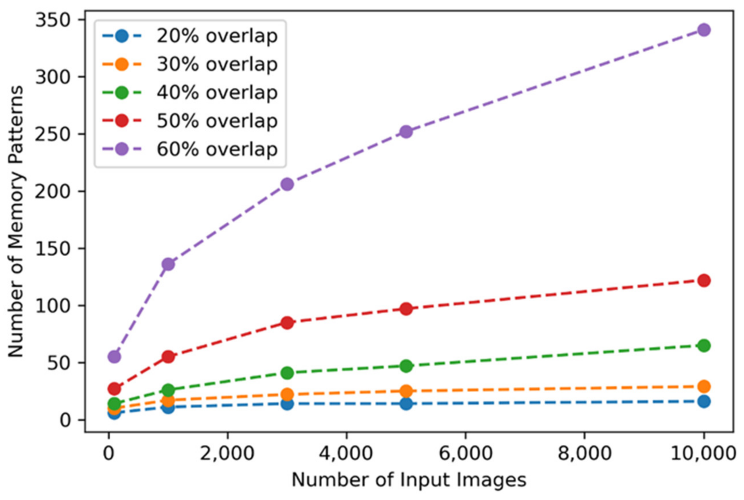
| 20% | 6 | 11 | 14 | 14 | 16 |
| 30% | 10 | 17 | 22 | 25 | 29 |
| 40% | 14 | 26 | 41 | 47 | 65 |
| 50% | 27 | 55 | 85 | 97 | 122 |
| 60% | 55 | 136 | 206 | 252 | 341 |
| Overlap Rate | 100 Images | 1000 Images | 3000 Images | 5000 Images | 9000 Images |
|---|---|---|---|---|---|
| 20% | 10 | 10 | 10 | 10 | 10 |
| 30% | 10 | 12 | 12 | 12 | 13 |
| 40% | 15 | 18 | 24 | 24 | 33 |
| 50% | 19 | 35 | 59 | 78 | 105 |
| 60% | 44 | 96 | 148 | 199 | 286 |
Publisher’s Note: MDPI stays neutral with regard to jurisdictional claims in published maps and institutional affiliations. |
© 2021 by the authors. Licensee MDPI, Basel, Switzerland. This article is an open access article distributed under the terms and conditions of the Creative Commons Attribution (CC BY) license (https://creativecommons.org/licenses/by/4.0/).
Share and Cite
Kang, K.; Bae, C. Memory Model for Morphological Semantics of Visual Stimuli Using Sparse Distributed Representation. Appl. Sci. 2021, 11, 10786. https://doi.org/10.3390/app112210786
Kang K, Bae C. Memory Model for Morphological Semantics of Visual Stimuli Using Sparse Distributed Representation. Applied Sciences. 2021; 11(22):10786. https://doi.org/10.3390/app112210786
Chicago/Turabian StyleKang, Kyuchang, and Changseok Bae. 2021. "Memory Model for Morphological Semantics of Visual Stimuli Using Sparse Distributed Representation" Applied Sciences 11, no. 22: 10786. https://doi.org/10.3390/app112210786
APA StyleKang, K., & Bae, C. (2021). Memory Model for Morphological Semantics of Visual Stimuli Using Sparse Distributed Representation. Applied Sciences, 11(22), 10786. https://doi.org/10.3390/app112210786