Constrained Multi-Objective Optimization of Simulated Tree Pruning with Heterogeneous Criteria

Abstract

Virtual pruning of simulated fruit tree models is a useful functionality provided by software tools for computer-aided horticultural education and research. It also enables algorithmic pruning optimization with respect to a set of quantitative objectives, which is important for analytical purposes and potential applications in automated pruning. However, the existing studies in pruning optimization focus on a single type of objective, such as light distribution within the crown. In this paper, we propose the use of heterogeneous objectives for discrete multi-objective optimization of simulated tree pruning. In particular, the average light intake, crown shape, and tree balance are used to observe the emergence of different pruning patterns in the non-dominated solution sets. We also propose the use of independent constraint objectives as a new mechanism to confine overfitting of solutions to individual pruning criteria. Finally, we perform the comparison of NSGA-II, SPEA2, and MOEA/D-EAM on this task. The results demonstrate that SPEA2 and MOEA/D-EAM, which use external solution archives, can produce better sets of non-dominated solutions than NSGA-II.

1. Introduction

Pruning is one of the most important horticultural intervention techniques with which the vegetative and reproductive growth of fruit trees can be balanced. This balance is important for producing a stable and high quality product in consecutive yield seasons [1,2]. Proper tree pruning also helps to prevent tree degradation, and reduces the chance of disease by providing sufficient light and air flow through the tree canopy [3]. The knowledge of tree pruning is, thus, an essential skill for both professional and amateur fruit growers. In recent years, a number of software tools have emerged for computer-aided horticultural education [4,5,6,7]. They complement the field training by allowing the user to perform various actions on simulated tree models within a 3D virtual environment. The effects of such interactive tree manipulation on its growth are simulated to provide an informative feedback to the user. The use of software tools can be extended beyond education, since they allow analysis and comparison of various tree training techniques.

Another functionality enabled by software is algorithmic determination and evaluation of pruning performed on virtual trees with respect to specific goals. Existing research in this direction includes goal-oriented assessment of pruning effects [8], selection of pruning points in 3D tree reconstructions from images or point clouds as part of automated pruning [9,10,11], and algorithmic pruning optimization for support in computer-aided education [12]. In a previous study, the immediate and delayed effects of selective pruning on fruit tree development were assessed using the estimated amount of light received by the flower buds in the current and the next season [13]. In this case, the light intake was a proxy measure for the achieved ratio of vegetative and reproductive growth resulting from pruning, which was the object of optimization. It was shown that pre-growth and post-growth evaluation of a single metric can result in a complex bi-objective optimization problem with conflicting goals.

The limitation of existing approaches to tree pruning optimization is that they are focused on a single pruning objective, which is the improvement of lighting conditions in the crown. Only Westling et al. [11] used the crown volume as an additional component in the calculation of the pruned tree’s final score. The problem of light intake maximization was approached from the perspective of both single-objective [12] and multi-objective optimization [13]. However, in the latter case, the objectives were homogeneous and their values were computed by the same function in different value spaces (after pruning and after regrowth). In practice, however, the objectives of pruning can reflect various additional goals, such as maintaining a desirable tree shape, volume, or balance [14]. In this paper, we propose and evaluate the multi-objective pruning optimization with such heterogeneous criteria, which are evaluated on the same pruned model. This extends to the existing methodology by including diverse goals considered in manual pruning, and provides new educational and analytical functionality for the optimization framework, which is implemented within the EduAPPLE virtual tree simulation tool [15].

Multi-objective optimization (MO) problems arise in many real-life and scientific tasks. Research of MO methods has produced a large number of efficient algorithms, which were used to solve practical problems ranging from groundwater remediation [16] to workload balancing [17]. Multi-objective problems can be approached using scalarization, Pareto-based algorithms, or hybrid approaches [18]. Scalarization to single-objective problems can employ mature and competitive optimization methods for specialized tasks [19]. However, state-of-the art results in multi-objective optimization problems were achieved by Pareto-based algorithms, which construct an approximation of a Pareto-optimal set of solutions [20]. Improved versions of baseline algorithms address the problems of poor solution diversity and premature convergence using crowding mechanisms [21,22], dynamic archives [23], or local exploration techniques [24].

In the paper, we analyze and compare the performance of the NSGA-II [25], the SPEA2 [26], and the MOEA/D-EAM [27] methods for pruning optimization in a 3D objective space. The objectives reflect the immediate effects of selective limb removal on light intake, crown symmetry, and the balance of a tree. We additionally propose the use of constraint objectives as a new regulative mechanism for reducing the overfitting of pruning solutions to individual objectives. The main contributions of this paper are:

• Integration of multiple heterogeneous objectives into a multi-objective tree pruning optimization framework.
• Introduction of secondary objectives, which are not the targets of optimization, but serve as constraints in the objective space of pruning solutions.
• Comparison and analysis of Pareto front approximations obtained with three popular advanced MO methods, namely NSGA-II, SPEA2, and MOEA/D-EAM.

2. Materials and Methods

In this section, we briefly review the tree growth simulation model, and describe the way pruning is formulated as an MO problem. We then define the new set of heterogeneous quantitative objectives for the pruning optimization problem, and describe the proposed constrained MO procedure.

2.1. EduAPPLE Tree Growth Simulator

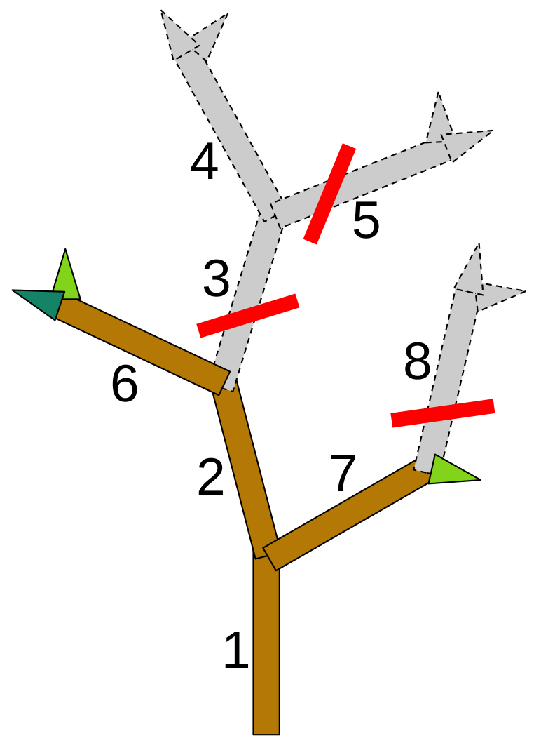
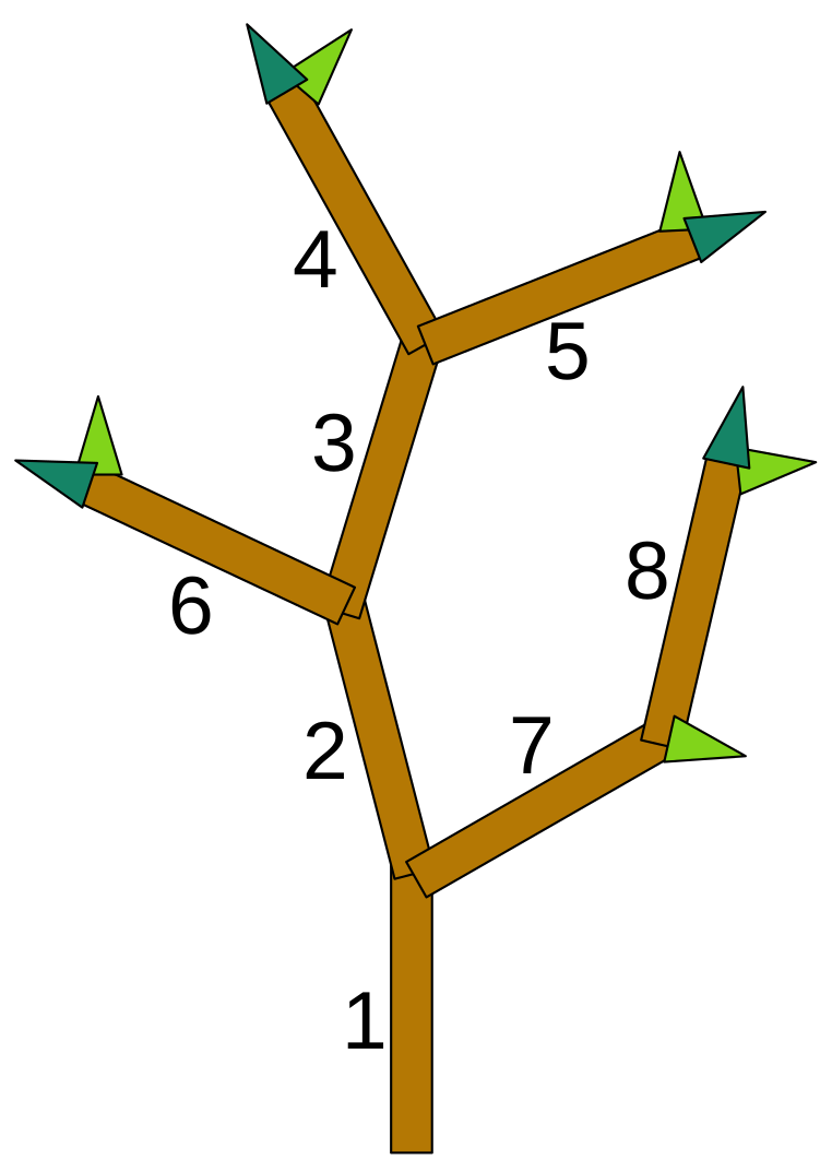
Tree growth simulator EduAPPLE [7,15] was developed as a software tool that allows the user to observe the effects of various tree training techniques, such as pruning, weighing, and spreading, on the formation of an apple tree crown. To this end, EduAPPLE implements a parameterized development model that allows simulation of different growth behaviors of apple trees. EduAPPLE uses a simplified tree structure representation, where the tree skeleton is composed of short linear segments called metamers, which are linked to form branches. Metamers also present the basic unit of increment in growth simulation. Each metamer consists of an internode and two buds, a terminal and a lateral one, which are used to extend or fork new branches upon growth. Internodes have assigned unique identifiers, which are used to indicate the cut locations for pruning. Figure 1 shows an example of a simple tree structure with depth-order internode labeling.

Simulation of tree growth in EduAPPLE is based on a source-sink model, and performed in discrete seasonal steps. The yearly increments are determined by first calculating the growth resources accumulated by a tree, and then redistributing them to different parts of the tree. The growth is realized by replacing the shooting buds with new metamers. The main sources of growth material are the tree’s own food reserves and photosynthesis. The amount of food reserve is modeled in EduAPPLE as a linear dependency on tree age A, while the quantity of photosynthetic product is estimated from total bud illuminance $q_i$:

$$R=C_1\min \{A,12\}+\left(C_2\tanh \left(\frac{0.2}{A}\right)+2\right)\sum _{i\in B}{q}_i.$$

(1)

Here, $B$ denotes the set of all buds, while $C_1$ and $C_2$ are adjustable model parameters. The hyperbolic tangent non-linearity is used to limit the tree growth with age. Bud illuminance is computed by estimating the amount of shadow the bud receives from other tree elements. The details of this calculation can be found in the original EduAPPLE paper [15].

Following the allocation theory [28], the accumulated resources R are split into two exclusive portions, which are dedicated separately to vegetative and reproductive growth. The estimated reproductive requirements of a tree are calculated using the number $N_f$ of flower buds as [13]:

$$r_{\mathrm{f}}=N_{\mathrm{f}}(C_3-C_4\times A).$$

(2)

Here, $C_3$ and $C_4$ are the allocation model parameters that can be adjusted to obtain specific behavior. The rest of the resources are allocated to vegetative growth. The reproductive pressure on resources can be reduced by pruning, which controls the balance of reproductive and vegetative growth across seasons.

Once determined, the vegetative growth resources are redistributed back to the buds in proportion to their light exposure, orientation, and distance from the roots. The probability of shooting is higher for well lit and vertically oriented buds, but reduced for older buds. Given the final amount $r_i$ of growth resources, bud i can sprout a sequence of $\lfloor r_i\rfloor$ new metamers. Upon creation, new buds are differentiated into vegetative and flowering ones, where the probability $p_f$ of a bud becoming a flowering one is another model parameter.

2.2. Pruning as an Optimization Problem

Algorithmic pruning optimization was introduced as an analytic tool by Strnad and Kohek [12]. In this context, a pruning is represented as a vector $\mathit{x}=\langle x_1,x_2,\dots ,x_n\rangle$ of cut locations, which correspond to individual internode identifiers. An example of this is shown in Figure 2, which illustrates the realization of a pruning vector for a given tree model. Figure 2 also shows that a cut can have no effect if another cut is present higher up in the tree hierarchy. This behavior is actually helpful during optimization, where changes to the pruning vector can activate and deactivate individual cuts.

The task of pruning optimization is to find a pruning solution that maximizes the values of selected quantitative objectives. Maximization of one objective, however, may result in a reduction of another objective. For instance, optimizing the crown shape towards some desired form may reduce the total resource accumulation of the tree, which affects the balance of vegetative and reproductive growth. Such conflict of goals is at the heart of multi-objective optimization proposed in this paper.

Let us formalize the pruning optimization problem with respect to a given set of objective functions $\mathit{f}=(f_1,\dots ,f_m)$. The objective value of a pruning solution vector $\mathit{x}$ is, in this case, given by $\mathit{f}\left(\mathit{x}\right)=(f_1\left(\mathit{x}\right),\dots ,f_m\left(\mathit{x}\right))$. A solution vector ${\mathit{x}}_i$ is said to be dominated by another solution vector ${\mathit{x}}_j$, which is denoted by ${\mathit{x}}_j\succ {\mathit{x}}_i$, if the following conditions hold:

• $\forall k\in [1,m]:f_k\left({\mathit{x}}_j\right)\ge f_k\left({\mathit{x}}_i\right)$;
• $\exists k\in [1,m]:f_k\left({\mathit{x}}_j\right)>f_k\left({\mathit{x}}_i\right)$.

In other words, pruning ${\mathit{x}}_j$ dominates pruning ${\mathit{x}}_i$ if it is not worse in any objective, and is strictly better in at least one. Note that the above formulation of dominance corresponds to the case of objective maximization used in this paper. For the minimization case, one needs to invert the inequalities.

The goal of MO is to construct a set $\mathcal{X}=({\mathit{x}}_1,{\mathit{x}}_2,\dots ,{\mathit{x}}_q)$ of non-dominated pruning solutions, known as the Pareto front. Only an approximation of the Pareto front can usually be obtained in practical problems. For this task, one can choose between several MO algorithms [29]. In this paper, the adaptations of three popular and efficient evolutionary MO methods were employed, known as NSGA-II [25], SPEA2 [26], and MOEA/D-EAM [27]. The latter is an extension of the original MOEA/D [30] method with a modified selection scheme that uses an external archive. In the terminology of evolutionary algorithms, the pruning solution vectors correspond to the genotypes, and their realizations on a tree model correspond to phenotypes. During the pruning optimization, the search is conducted in the genotype space, while the fitness evaluation is performed in the phenotype space.

2.3. Objectives

In a previous study by Strnad et al. [13], the bi-objective value of a pruning solution $\mathit{x}$ for a given tree model $\mathcal{T}$ was defined using the pre-growth objective value $f_{\mathrm{pre}}$ and the post-growth objective value $f_{\mathrm{post}}$:

$$\mathit{f}\left(\mathit{x}\right)=(f_{\mathrm{pre}}\left({\mathcal{T}}_{/\mathit{x}}\right),f_{\mathrm{post}}\left({\mathcal{T}}_{/\mathit{x}}\right)).$$

(3)

The quantity $f\left({\mathcal{T}}_{/\mathit{x}}\right)$ is the estimated light intake of a tree $\mathcal{T}$ after being pruned according to $\mathit{x}$. The pre-growth objective $f_{\mathrm{pre}}$ reflects the short-term (i.e., immediate) effects of pruning, which can be assessed directly on the pruned tree model. On the other hand, the post-growth objective $f_{\mathrm{post}}$ serves as a proxy measure for long-term (i.e., delayed) pruning effects. These are estimated by averaging the light intake over the results of multiple stochastic growth simulations of the pruned tree.

Improving the light conditions within the crown is one of the principal goals of tree pruning. However, there are other important aspects that practitioners need to consider, especially when performing the pruning as a corrective measure in neglected or damaged trees. For example, the amount of removed biomass may need to be constrained in order to prevent inflicting too much stress on the tree, or the disrupted tree balance needs to be restored by improving biomass distribution. Such heterogeneous criteria can constitute conflicting objectives for the pruning optimization task. In this paper, we analyze the results of such multi-objective optimization by introducing the following pruning objectives:

• The average light exposure of flower buds after pruning, denoted by $f_1$, and calculated as:

  $$f_1\left(\mathit{x}\right)=\frac{1}{N_f}\sum _{i\in B_{\mathrm{f}}\left({\mathcal{T}}_{/\mathit{x}}\right)}{q}_i^2.$$

  (4)

  Here, $B_{\mathrm{f}}\left({\mathcal{T}}_{/\mathit{x}}\right)\subset B\left({\mathcal{T}}_{/\mathit{x}}\right)$ denotes the set of the pruned tree’s flower buds. Note that this objective promotes aggressive pruning, since the maximum value can be achieved by a few fully exposed buds.
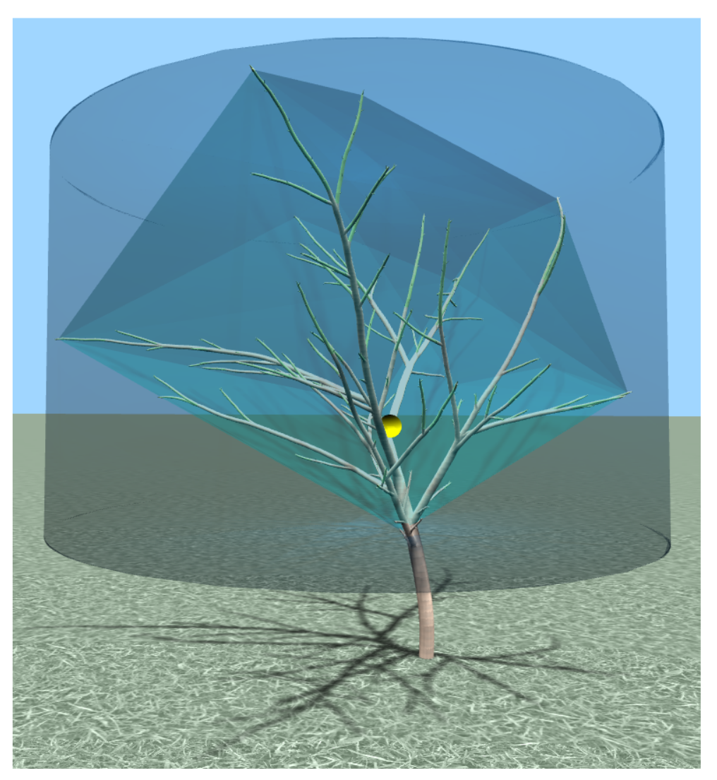
• Conformance of crown shape to the desired training form, which is denoted by $f_2$. Its value is estimated using the inverse Hausdorff distance between the convex hull of the pruned tree and the hull’s bounding volume of target symmetric shape:

  $$f_2\left(\mathit{x}\right)=h^{-1}(\mathcal{H}\left({\mathcal{T}}_{/\mathit{x}}\right),\mathcal{C}\left({\mathcal{T}}_{/\mathit{x}}\right)).$$

  (5)

  The convex hull $\mathcal{H}$ of the pruned tree is constructed using its branch tips. Once the hull is obtained, its bounding volume $\mathcal{C}$ with target shape is determined (Figure 3). In our experiments, a cylindrical target shape was pursued, but other common training forms can be used (e.g., conical). The Hausdorff distance between two shapes is defined as:

  $$h(X,Y)=\max \{\underset{x\in X}{\sup }\underset{y\in Y}{\inf }d(x,y),\underset{y\in Y}{\sup }\underset{x\in X}{\inf }d(x,y)\},$$

  (6)

  where d denotes the standard Euclidean distance between two points.
• Tree balance, denoted by $f_3$, and represented by the inverse horizontal distance $d_{\mathit{c}}$ between the above ground biomass center of gravity $\mathit{c}$ and the vertical axis going through the stem origin:

  $$f_3\left(\mathit{x}\right)=\frac{1}{1+d_{\mathit{c}}}.$$

  (7)
  The center of gravity location $\mathbf{c}$ for a tree ${\mathcal{T}}_{/\mathit{x}}$ with internodes $\mathcal{I}\left({\mathcal{T}}_{/\mathit{x}}\right)$ is computed as:

  $$\mathit{c}=\frac{{\displaystyle \sum _{i\in \mathcal{I}\left({\mathcal{T}}_{/\mathit{x}}\right)}}{m}_i{\mathit{s}}_i}{\sum _{i\in \mathcal{I}\left({\mathcal{T}}_{/\mathit{x}}\right)}{m}_i}.$$

  (8)
  Here, ${\mathit{s}}_i$ is the midpoint of internode i, and $m_i$ is its mass. The computation of the latter is simplified by assuming homogeneous wood density, so the mass of internode i with radius $r_i$ and length $l_i$ is proportional to its cylindrical volume:

  $$m_i=l_i{r}_i^2.$$

  (9)
• The proportion of remaining tree biomass, denoted by $f_4$ and calculated as:

  $$f_4\left(\mathit{x}\right)=\frac{m\left({\mathcal{T}}_{/\mathit{x}}\right)}{m\left(\mathcal{T}\right)}.$$

  (10)
  Here, $m\left(\mathcal{T}\right)$ is the above ground biomass of tree $\mathcal{T}$:

  $$m\left(\mathcal{T}\right)=\sum _{i\in \mathcal{I}\left(\mathcal{T}\right)}{m}_i.$$

  (11)

2.4. Optimization Method

In this paper, pruning optimization is treated as a discrete combinatorial optimization problem, where the task is to find the set $\mathcal{X}$ of non-dominated pruning solution vectors with respect to a set of objectives $\mathit{f}=(f_1,f_2,f_3)$. Objective $f_4$, defined in Section 2.3, is itself not an interesting target of optimization, since it can be maximized trivially by no pruning at all. Therefore, we propose a special role for objective $f_4$ in order to constrain the search to certain regions of the solution space. For instance, we may prescribe that no more than $10\%$ of the tree’s biomass should be removed, which could be imposed by the constraint $f_4>0.9$. This is especially important in order to regulate aggressive pruning stimulated by objective $f_1$. Adherence to constraint objective bounds is implemented in a soft manner by marking the violating solutions as dominated. Such approach does not completely reject borderline solutions, making it possible to use them for the derivation of better successors. We use only $f_4$ as a constraint objective in this study, but other metrics could be used. The distinctive property of a constraint objective is that it evaluates the pruning solution globally, and not with respect to individual cuts. In general, both the lower and the upper bounds for a constraint objective can be specified by the user.

The use of constraint objectives to specify feasible regions in an auxiliary objective space is a new addition to the multi-objective pruning optimization framework, which complements heuristic constraints implemented in a decision space. The latter have been introduced by Strnad et al. [13] in order to reduce the size of the solution space and make the search more efficient. This is achieved by two mechanisms:

• By limiting the cut locations to those with certain local properties. In our tests, the following restrictions were enforced:

  -

  Cutting was limited to the wood at most $A_{\max }$ years old, in order to prevent pruning of scaffold limbs.

  -

  Pruning was restricted to locations following a branch fork that result in removal of at least $m_{\min }$ metamers.

• By constraining the dimension of the solution vectors (i.e., the number of cuts) to a range $[d_{\min },d_{\max }]$.

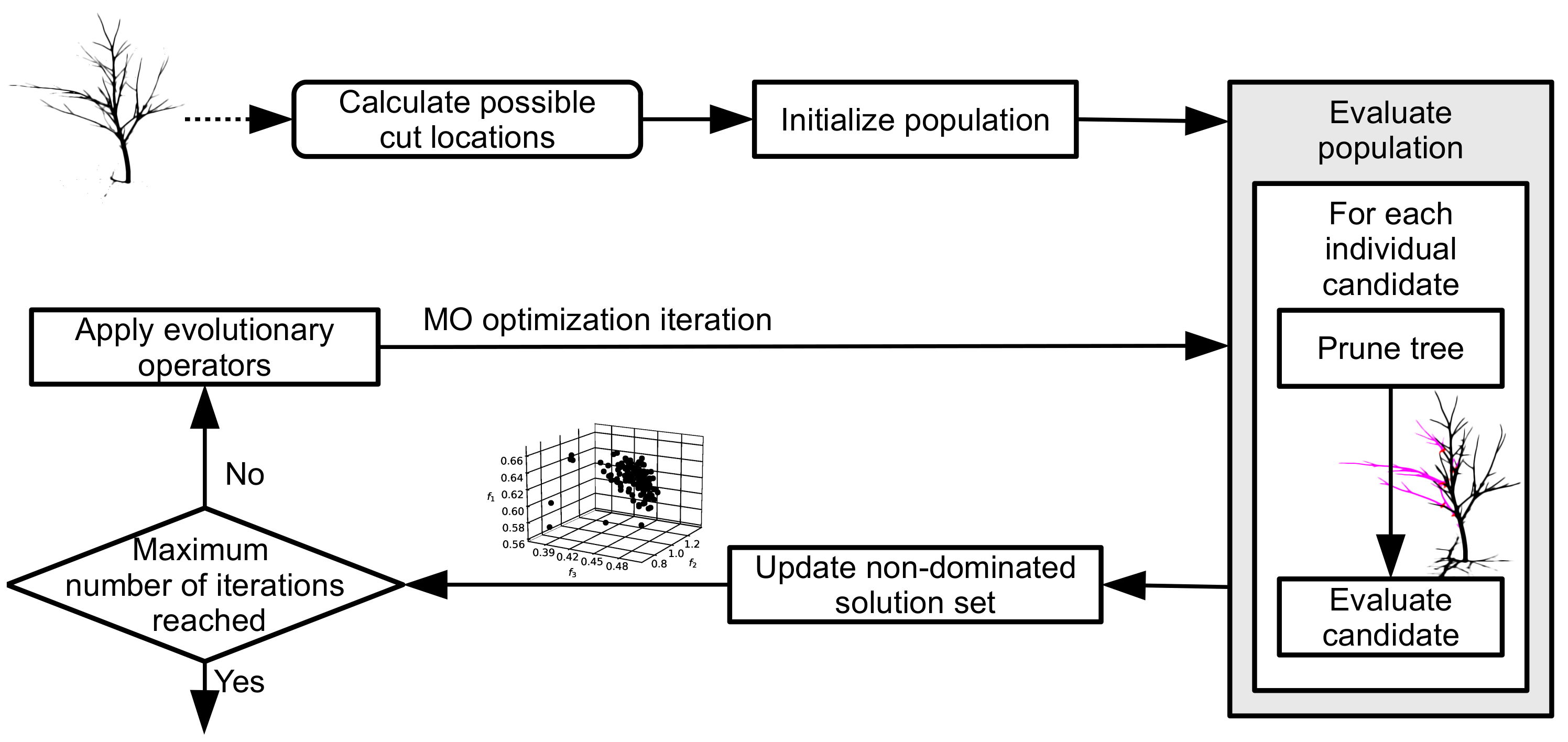
The high-level concept of the proposed multi-objective pruning optimization is outlined in Figure 4 and Algorithm 1. It is an adaptation of a general evolutionary process for the construction of Pareto front approximation. Given a tree model $\mathcal{T}$ as input, a list ${\mathcal{I}}_{\mathrm{cut}}\left(\mathcal{T}\right)\subset \mathcal{I}\left(\mathcal{T}\right)$ of potential cut locations is first built according to the heuristic constraints described above. From this list, the initial population ${\mathcal{P}}^{\left(0\right)}=\left\{{\mathit{x}}_i^{\left(0\right)}\right\}$ of $Ps$ solution vectors is generated. Each solution vector is obtained by sampling d-times randomly and without replacement from ${\mathcal{I}}_{\mathrm{cut}}\left(\mathcal{T}\right)$, where $d\in [d_{\min },d_{\max }]$. The population size $Ps$ is a method meta-parameter.

Algorithm 1. Multi-objective pruning optimization.

Input: Tree model $\mathcal{T}$; heuristic constraints $[d_{\min },d_{\max }]$, $A_{\max }$, and $m_{\min }$; number of objective evaluations M; objective functions $\mathit{f}$; meta-parameters $Ps,Cr,Mr,\mathit{P}$ Output: non-dominated set of solutions $\mathcal{X}$ 1: procedureMO($\mathcal{T},d_{\min },d_{\max },A_{\max },m_{\min },M,\mathit{f},Ps,Cr,Mr,\mathit{P}$) 2:     ${\mathcal{I}}_{\mathrm{cut}}\leftarrow$ list of possible cut locations in $\mathcal{T}$ according to $[d_{\min },d_{\max }]$, $A_{\max }$, and $m_{\min }$ 3:     ${\mathcal{P}}^{\left(0\right)}\leftarrow$ initial population of random vectors ${\mathit{x}}_i^{\left(0\right)}(i=1,\dots ,Ps)$ sampled from ${\mathcal{I}}_{\mathrm{cut}}$ 4:     $\mathcal{X}\leftarrow \varnothing$ 5:     for $k=0\dots M/Ps$ do 6:         for $\forall {\mathit{x}}_i^{\left(k\right)}\in {\mathcal{P}}^{\left(k\right)}$ do 7:            ${\mathcal{T}}_{/\mathit{x}}\leftarrow$ prune $\mathcal{T}$ according to ${\mathit{x}}_i^{\left(k\right)}$ 8:            ${\mathit{f}}_i\left({\mathit{x}}_i^{\left(k\right)}\right)\leftarrow$ evaluate $\mathit{f}$ on ${\mathcal{T}}_{/\mathbf{x}}$ 9:         $\mathcal{Y}\leftarrow$ non-dominated vectors in ${\mathcal{P}}^{\left(k\right)}$ 10:         $\mathcal{Y}\leftarrow$ remove vectors from $\mathcal{Y}$ that violate bounds of constraint objective $f_4$ 11:         update $\mathcal{X}$ using $\mathcal{Y}$ 12:         ${\mathcal{P}}^{(k+1)}\leftarrow$ apply evolutionary operators on ${\mathcal{P}}^{\left(k\right)}$ using $Cr,Mr$ and $\mathit{P}$ 13:     return $\mathcal{X}$

The procedure then enters the optimization loop. The number of iterations N is either specified directly, or calculated from the maximum number of objective evaluations M as $N=\frac{M}{Ps}$. Within the loop, three main steps are performed:

• The current population ${\mathcal{P}}^{\left(k\right)}=\left\{{\mathit{x}}_i^{\left(k\right)}\right\}$ is evaluated according to objectives $\mathit{f}$.
• The set of non-dominated solutions is updated, using the constraint objective $f_4$ to demote unsuitable solutions.
• The next generation of solutions is produced by applying evolutionary operators to the current population.

Evaluation of individual candidate solution ${\mathit{x}}_i$ is performed by pruning the tree model according to ${\mathit{x}}_i$, and computing the values of objectives on the resulting pruned tree. This part of the computation is performed by the simulation model, and is independent of the used optimization algorithm.

The set $\mathcal{X}$ of non-dominated pruning solutions is updated next, which is a step that depends on the evolutionary method used. In NSGA-II, $\mathcal{X}$ is updated with non-dominated solutions from the current population ${\mathcal{P}}^{\left(k\right)}$. In SPEA2 and MOEA/D-EAM, the current archive ${\overline{\mathcal{P}}}^{\left(k\right)}$ is used to update $\mathcal{X}$ in each iteration. In both cases, solutions with objective value $f_4$ below the prescribed limit are not included in $\mathcal{X}$ even if non-dominated.

The last step is the derivation of a new population ${\mathcal{P}}^{(k+1)}$ from the current population ${\mathcal{P}}^{\left(k\right)}$ using a method-dependent procedure. In all of our experiments, the following problem-specific implementations of evolutionary operators are used:

• Selection of two parent vectors from the population (NSGA-II) or the mating pool (SPEA2 and MOEA/D-EAM).
• Uniform crossover of parent vectors with probability $Cr$.
• Mutation of child vectors with change probabilities $\mathit{P}=\langle P_{\mathrm{move}},P_{\mathrm{add}},P_{\mathrm{remove}}\rangle$ and mutation rate $Mr$.

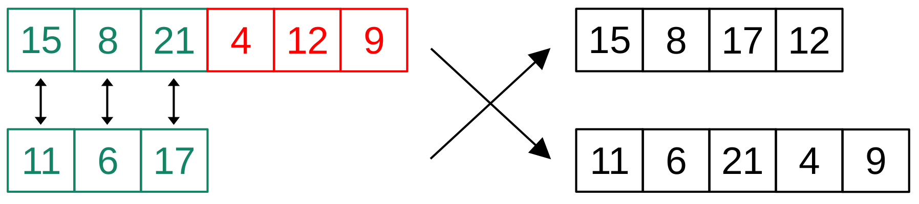
The selection step is method-dependent. In NSGA-II [25] and SPEA2 [26], binary tournaments are used to select the parents from the population and the mating pool, respectively. The mating pool is also used by MOEA/D-EAM [27], but its selection scheme combines random selection with a neighborhood-based one. During crossover, special consideration is necessary when recombining parent vectors of different sizes. In such cases, the surplus genes of the longer parent vector are distributed uniformly between the two child vectors (Figure 5). Mutation of a child vector is performed in two steps. First, a randomly selected cut is relocated to a different valid position from ${\mathcal{I}}_{\mathrm{cut}}\left(\mathcal{T}\right)$ with probability $P_{\mathrm{move}}$, removed from pruning with probability $P_{\mathrm{remove}}$, or added to pruning with probability $P_{\mathrm{add}}$. Cut addition and removal are possible only if the size of the resulting pruning vector remains within the range $[d_{\min },d_{\max }]$. In the second phase, all of the other cuts are replaced by randomly selected alternatives with small probability $Mr$. The complete implementation of crossover and mutation is shown in Algorithm 2.

The exploration/exploitation behavior of the search is regulated through meta-parameters $Cr,Mr$, and $\mathbf{P}$. Sufficient exploration can usually be achieved even with small values of crossover and mutation rates, because local changes of a genotype (i.e., pruning vector) can result in significantly different phenotypes (i.e., pruned tree models).

Algorithm 2. Implementation of crossover and mutation.

Input: parent vectors ${\mathit{x}}_1$ and ${\mathit{x}}_2$, crossover rate $Cr$, mutation rate $Mr$, change probability distribution $\mathit{P}=\langle P_{\mathrm{move}},P_{\mathrm{add}},P_{\mathrm{remove}}\rangle$, vector length constraints $d_{\min }$ and $d_{\max }$ Output: offspring vector $\mathit{y}$ 1: procedureGenerate_child(${\mathit{x}}_1,{\mathit{x}}_2,Cr,Mr,\mathit{P},d_{\min },d_{\max }$) 2:     if rand() < $Cr$ then 3:         $l_1\leftarrow \mathrm{length}\left({\mathit{x}}_1\right)$, $l_2\leftarrow \mathrm{length}\left({\mathit{x}}_2\right)$ 4:         for $i=1\dots \min (l_1,l_2)$ do 5:            $\mathit{y}\left[i\right]\leftarrow \left\{\begin{array}{cc}{\mathit{x}}_1\left[i\right]& \mathrm{if} rand\left(\right)<0.5\hfill \\ {\mathit{x}}_2\left[i\right]& \mathrm{otherwise}\hfill \end{array}\right.$ 6:         for $i=\min \left(l_1,l_2\right)+1\dots \max \left(l_1,l_2\right)$ do 7:            if rand() < 0.5 then 8:                $\mathit{y}[\mathrm{length}\left(\mathit{y}\right)+1]\leftarrow \left\{\begin{array}{cc}{\mathbf{x}}_1\left[i\right]& \mathrm{if} l_1>l_2\hfill \\ {\mathit{x}}_2\left[i\right]& \mathrm{otherwise}\hfill \end{array}\right.$ 9:     else 10:         $\mathit{y}\leftarrow \left\{\begin{array}{cc}{\mathit{x}}_1& \mathrm{if} rand\left(\right)<0.5\hfill \\ {\mathbf{x}}_2& \mathrm{otherwise}\hfill \end{array}\right.$ 11:     $l\leftarrow \mathrm{length}\left(\mathit{y}\right)$ 12:     if $l=d_{\min }$ then 13:         $P_{\mathrm{remove}}\leftarrow 0$ 14:     else if $l=d_{\max }$ then 15:         $P_{\mathrm{add}}\leftarrow 0$ 16:     re-normalize $\mathit{P}$, $r\leftarrow \mathrm{rand}(1,l)$ 17:     if $r<P_{\mathrm{remove}}$ then 18:         remove $\mathit{y}\left[\mathrm{rand}\right(1,l\left)\right]$ from $\mathit{y}$ 19:     else if $r<P_{\mathrm{remove}}+P_{\mathrm{add}}$ then 20:         $\mathit{y}[l+1]\leftarrow {\mathcal{I}}_{\mathrm{cut}}\left[\mathrm{rand}\right(1,|{\mathcal{I}}_{\mathrm{cut}}\left|\right)]$ 21:     else 22:         $j\leftarrow \mathrm{rand}(1,l)$ 23:         $\mathit{y}\left[j\right]\leftarrow {\mathcal{I}}_{\mathrm{cut}}\left[\mathrm{rand}\right(1,|{\mathcal{I}}_{\mathrm{cut}}\left|\right)]$ 24:         for $i=1\dots l,i\ne j$ do 25:            if rand() < $Mr$ then 26:                $\mathit{y}\left[i\right]\leftarrow {\mathcal{I}}_{\mathrm{cut}}\left[\mathrm{rand}\right(1,|{\mathcal{I}}_{\mathrm{cut}}\left|\right)]$ 27:     return $\mathit{y}$

3. Results

The goals of the experiments presented in this section are to:

• Determine the properties of Pareto front approximations obtained from pruning optimization with multiple heterogeneous objectives. In particular, we are interested in the relation of generated pruning solutions to three reference proposals, corresponding to non-pruning, non-selective pruning to cylindrical shape, and distance-based pruning, where the secondary branches are removed if their distance to the primary ones is below the threshold.
• Investigate the pruning patterns produced by MO, and how they reflect the trade-offs between conflicting pruning goals.
• Evaluate the effect of the proposed constraint objectives on the resulting Pareto front approximations and solution characteristics.
• Compare the performance of NSGA-II, SPEA2, and MOEA/D-EAM on this problem, which is important from the perspective of future framework development.

In the continuation, we first describe the configuration and workflow of experiments, and then address the above research questions in order.

The hardware used for the experiments was a desktop computer with Intel i7 CPU, NVIDIA GeForce GTX 1060 GPU, and 16 GB of RAM. The software environment included the Linux operating system (kernel version $5.13.11$) and the GCC compiler version 11.1.

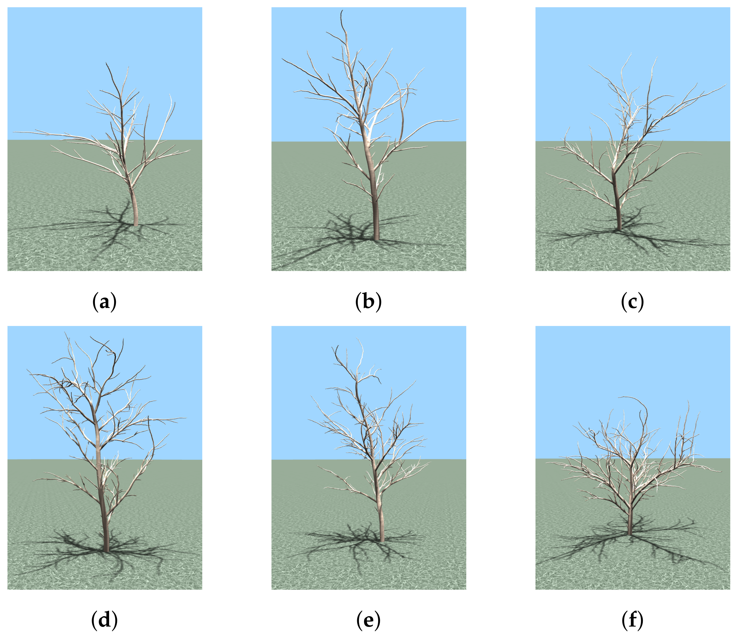
The tree models for experiments were generated by using the simulator with growth parameters $C_1=80,C_2=40,C_3=80,C_4=20$, and $p_f=0.08$. The models are shown in Figure 6, and present different levels of complexity for pruning optimization. Their main structural properties and the corresponding combinatorial search space sizes are reported in

Table 1. Characteristics of experimental tree models.

Tree Model	# of Intermodes	# of Potential Cut Locations	Search Space Size
Figure 6a	1121	161	$1.63\times {10}^{29}$
Figure 6b	1234	145	$9.75\times {10}^{27}$
Figure 6c	1919	253	$2.54\times {10}^{34}$
Figure 6d	2506	341	$5.92\times {10}^{37}$
Figure 6e	2647	354	$1.55\times {10}^{38}$
Figure 6f	3740	429	$2.18\times {10}^{40}$

.

Tuning of methods’ meta-parameters was performed with a grid search using the pools $Ps\in \{20,30,50,100\}$, $Mr\in \{0.01,0.03,0.05,1.0\}$, and $Cr\in \{0.7,0.8,0.9,1.0\}$. The best out of 5 optimization runs with 5000 objective evaluations was selected for each configuration. The configurations were ordered using the hypervolume indicator $I_H$ [31]. For NSGA-II and SPEA2, the configuration $Ps/Mr/Cr=50/0.05/0.8$ was the configuration with the highest $I_H$ value. Its performance was also stable across a selection of tree models, and was therefore used in the final experiments. For MOEA/D-EAM, a smaller $Ps=30$ and $Mr=0.03$ in combination with $Cr=1$ proved to be optimal. The MOEA/D-EAM uses additional neighborhood size $Ns$ parameter, which was set to the recommended value $Ps/10$. A wider neighborhood setting $Ns=Ps/5$ was also experimented with, but performed worse than the default.

In order to analyze the effects of individual meta-parameters in more detail, we used the ratio of non-dominated individuals (RNI) [32], which is computed between solution sets of the selected reference configuration and the modified configurations. The best solutions, in terms of RNI, were selected out of 5 optimization runs and used for configuration comparison. The effects of individual meta-parameters are reported in

Table 2. Analysis of meta-parameter effects on quality of non-dominated solution sets, measured by the RNI metric [32]. For each optimization method, the parameters $Ps$, $Mr$ and $Cr$ were individually modified. The RNI for a configuration with specific value of the observed parameter is computed with respect to other configurations using different values of the same parameter.

Method	Configuration $\mathrm{Ps}/\mathrm{Mr}/\mathrm{Cr}$	Parameter Value / RNI
NSGA-II	$Ps$	20	30	50	100
	$Ps/0.05/0.8$	0.579	0.667	0.971	0.875
	$Mr$	0.01	0.03	0.05	0.1
	$50/Mr/0.8$	0.636	0.679	0.857	0.676
	$Cr$	0.7	0.8	0.9	1.0
	$50/0.05/Cr$	0.750	0.771	0.692	0.696
SPEA2	$Ps$	20	30	50	100
	$Ps/0.05/0.8$	0.644	0.806	0.808	0.684
	$Mr$	0.01	0.03	0.05	0.1
	$50/Mr/0.8$	0.689	0.769	0.885	0.812
	$Cr$	0.7	0.8	0.9	1.0
	$50/0.05/Cr$	0.658	0.962	0.880	0.724
MOEA/D-EAM	$Ps$	20	30	50	100
	$Ps/0.03/1.0$	0.833	0.870	0.750	0.619
	$Mr$	0.01	0.03	0.05	0.1
	$30/Mr/1.0$	0.944	1.000	0.800	0.636
	$Cr$	0.7	0.8	0.9	1.0
	$30/0.03/Cr$	0.720	0.706	0.875	0.879

.

It can be observed that, for NSGA-II and MOEA/D-EAM, the selection of $Cr$ is less sensitive than for SPEA2. For NSGA-II, larger population sizes can be used than for the other two methods, while SPEA2 performs comparatively for population sizes 30 and 50. Because the canonical NSGA-II does not use an external archive, the initial diversity with a small population can be exhausted before a large enough pool of feasible non-dominated solutions can be constructed. MOEA/D-EAM prefers smaller mutation rates than NSGA-II and SPEA2 because the changes are propagated faster across the population via the neighborhood mechanism.

The probability mass function for different mutation types was taken from the study by Strnad et al. [13], where $\mathit{P}=\langle P_{\mathrm{move}},P_{\mathrm{add}},P_{\mathrm{remove}}\rangle =\langle 0.3,0.35,0.35\rangle$ performed well. Using equal probabilities for extending and shortening the solution vectors also encourages searching with mean pruning size. An empirical lower bound value $0.9$ was used for the constraint objective $f_4$, i.e., no more than $10\%$ of the tree’s biomass should be removed by pruning, which is a pragmatical limit. In order to reduce the search space and prevent negligible cuts, the same values for heuristic constraints $A_{\max }=4$ and $m_{\min }=10$ as in [13] were used. The number of cuts in a pruning solution was also constrained empirically to the range $[5,25]$.

The number of objective evaluations in the final experiments was set to $M=\mathrm{10,000}$. The NSGA-II, SPEA2, and MOEA/D-EAM optimization methods were executed $q=11$ times for each tree model. Within each method, the obtained q non-dominated sets were compared in order to determine the number of overall non-dominated solutions in them. The fronts were then sorted by the decreasing number of non-dominated solutions. The best, median, and worst run of both optimization methods were finally used in the analysis of results and method comparison.

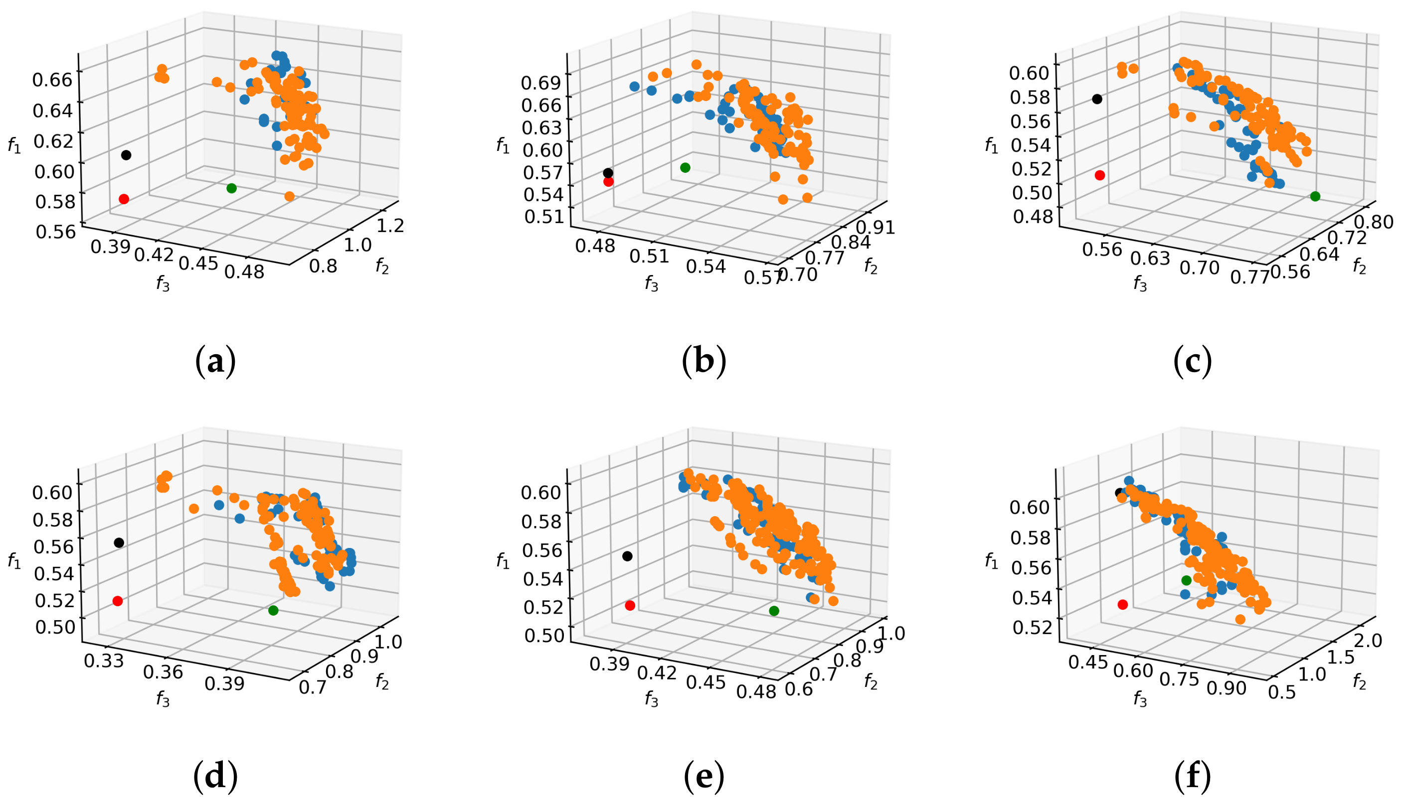
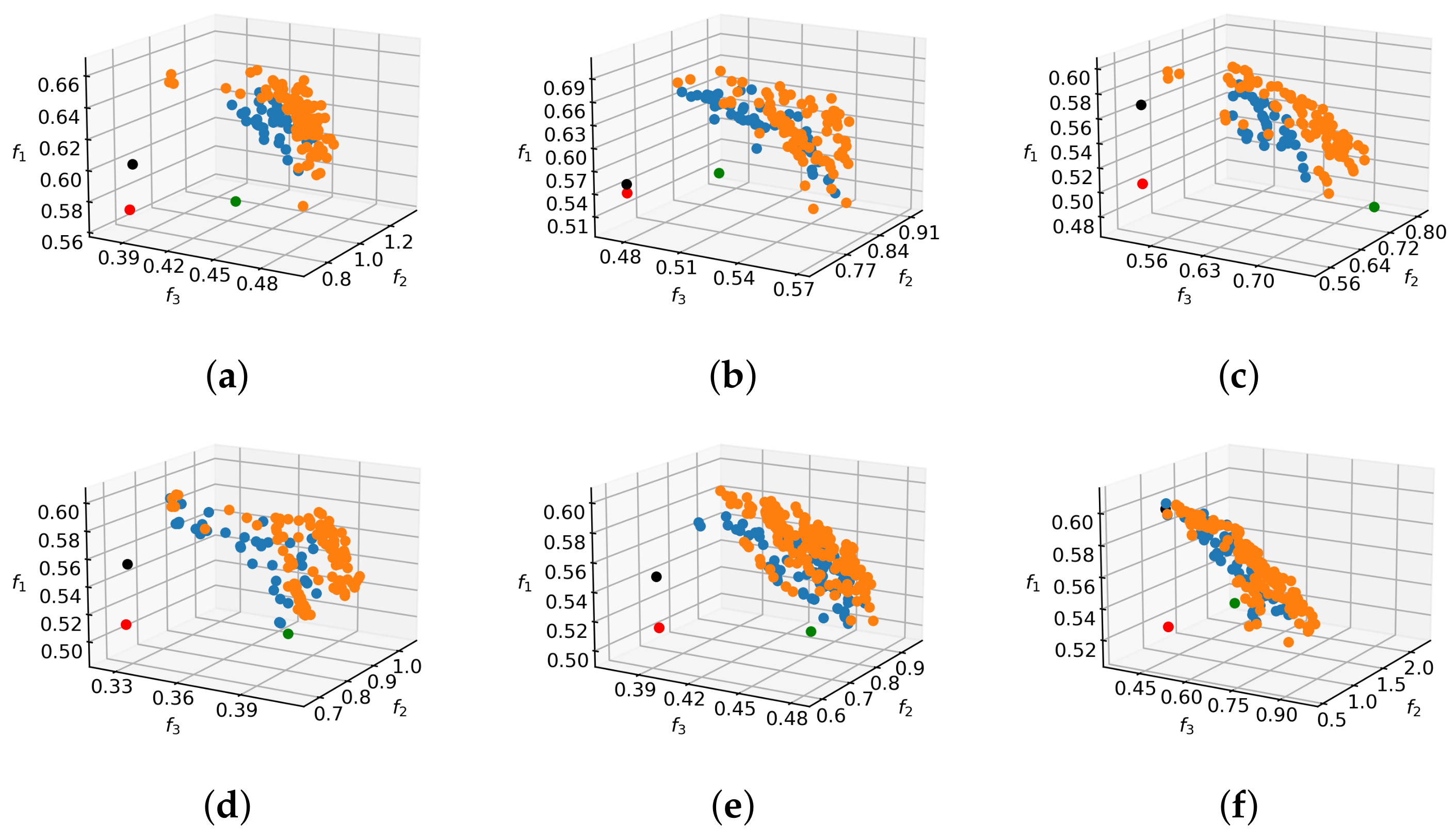
Figure 7 shows 3D approximations of Pareto fronts, obtained by the best runs of NSGA-II and SPEA2 for the tree models from Figure 6. Figure 8 shows the same comparison for MOEA/D-EAM and SPEA2.

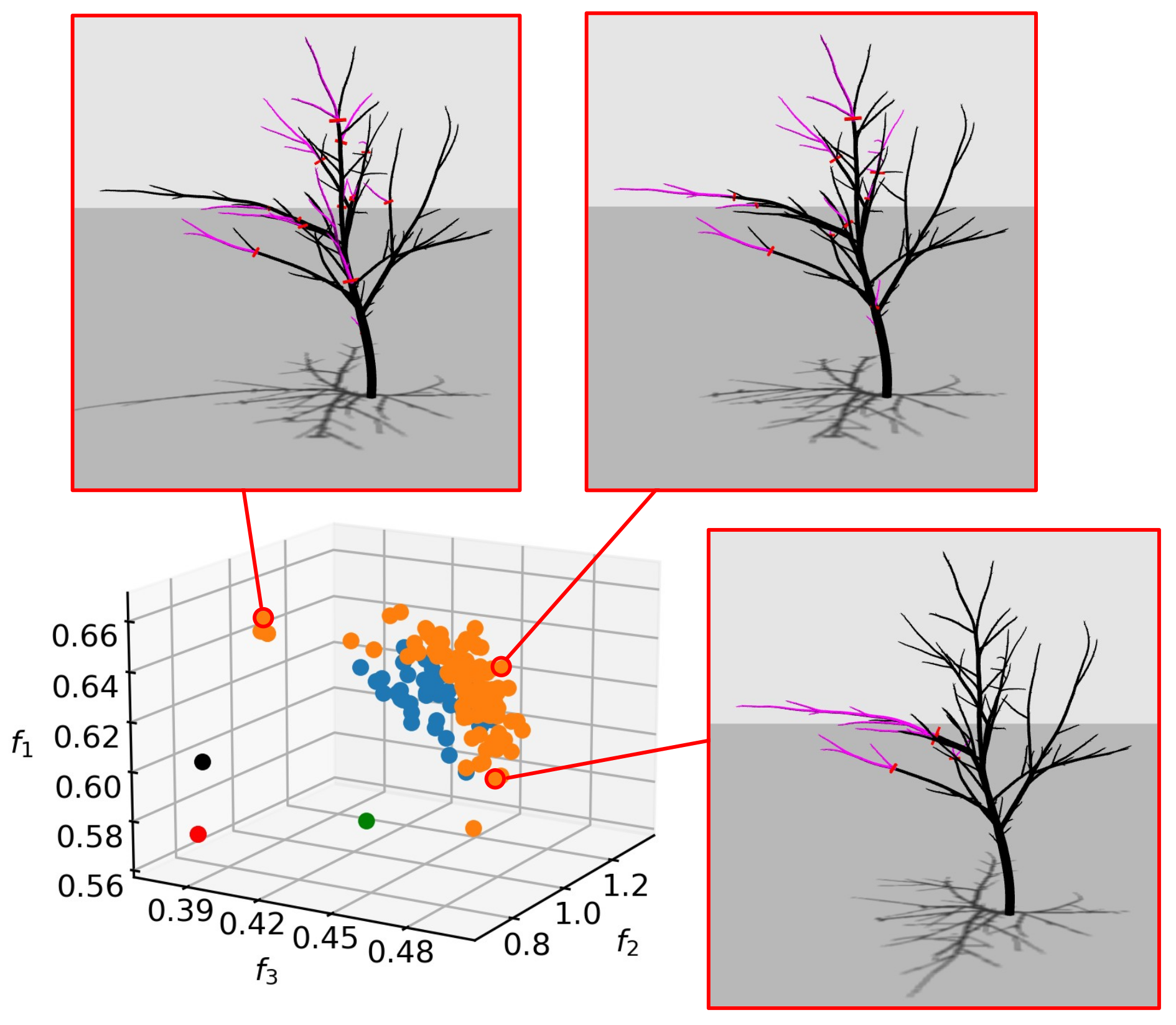
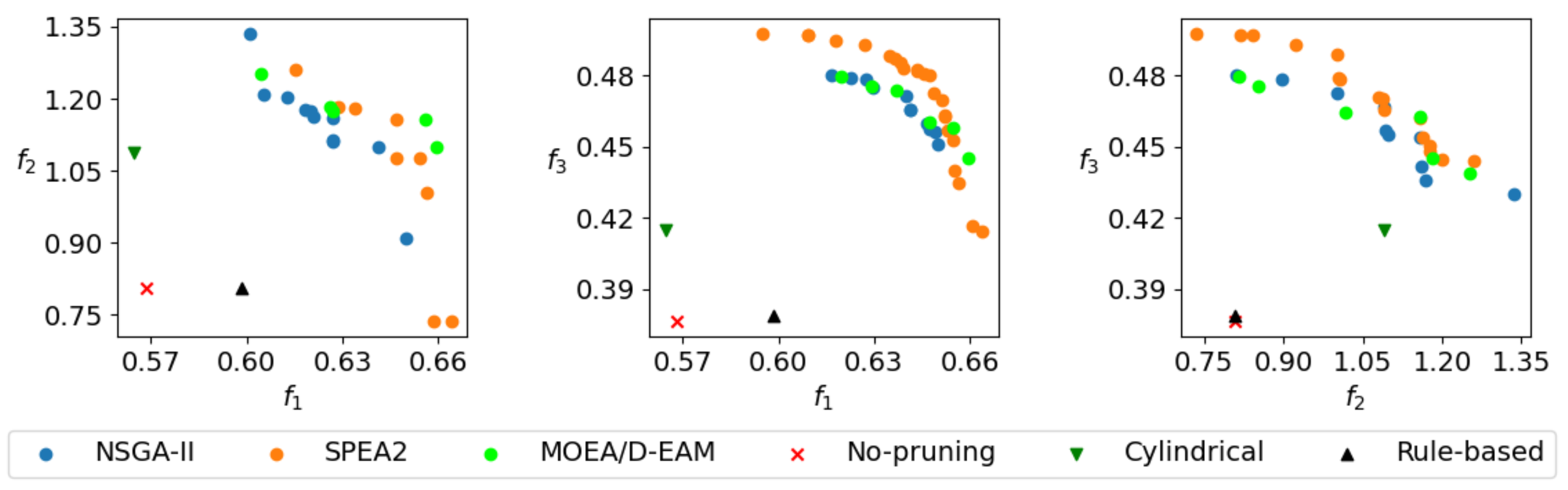
In order to convey a better sense of shape and relation to reference solutions, the 2D projections of the Pareto front approximation for the tree in Figure 6a are shown in Figure 9. The situation is similar for other tree models. It can be observed that all of the reference solutions are dominated by the majority of non-dominated individuals found by MO methods, because their positions in objective space projections are within the dominated regions behind the non-dominated fronts. As expected, the non-selective pruning to cylindrical form improves the value of objectives $f_2$ and $f_3$ with respect to no pruning, while the rule-based pruning increases the value of objective $f_1$. However, the results of pruning optimization demonstrate that simultaneous improvement on all objectives is possible. In relative terms, the hardest improvements to make are with respect to objective $f_1$. This can be explained by analyzing the behavior of that objective, which computes the average light exposure of flower buds. By pruning away branches, the number of buds that contribute to the objective value is reduced, but at the same time the light conditions for the remaining ones are improved and the denominator in Equation (4) is lowered. This gain vs. loss ratio of light intake can be highly discontinuous even for small changes in the solution vector, which results in multiple local optima that make optimization difficult.

Figure 10 shows realizations of pruning vectors from different regions of the non-dominated set on the target tree model. It is informative to compare the pruning solutions that focus on maximization of individual objectives. For example, the pruning that maximizes the light objective tends to remove branches that cast or receive a lot of shadow, whereas the balance-oriented pruning promotes one-sided removal of wood in order to restore tree equilibrium. The pruning solution focusing on shape objective $f_2$ advocates branch removal from multiple sides, but contains elements of the other two prunings in order to improve on objectives $f_1$ and $f3$ as well.

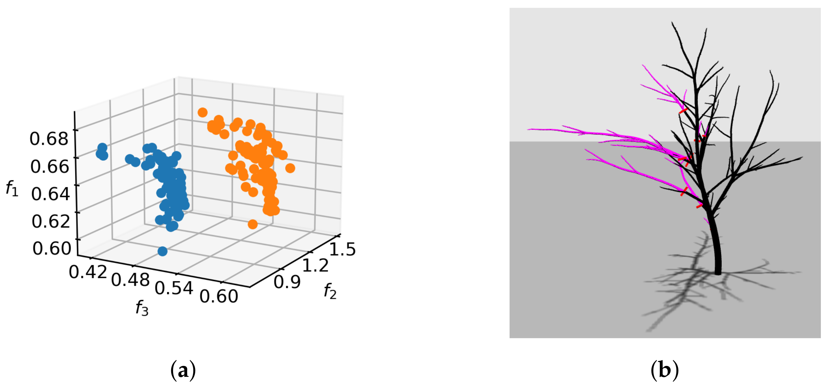
The next question addressed with the experiments was the evaluation of constraint objective $f_4$ importance for regulating the optimization. To this end, we executed the SPEA2 optimization using a relaxed lower bound $0.8$ for $f_4$. The comparison of non-dominated sets for the best SPEA2 run with tight and relaxed bound is shown in Figure 11a. It is evident that further numerical improvement of objective values can be achieved by relaxing the constraint. However, the solutions tend to start overfitting on one or more pruning objectives through extensive biomass removal (Figure 11b). A proper empirical selection of bounds is, thus, necessary to confine the solutions to viable regions.

Figure 11a shows that the effect of the constraint objective is in bounding the feasible region of the objective space. By relaxing the constraint, we allow a wider spread of individual objective values, which increases the possible distance of non-dominated fronts from the origin. Such indirect specification of feasible regions is in contrast to defining constraints in terms of optimization objectives themselves, which is more common in MO [33].

The final goal of experiments is comparison of method performance. Figure 7 suggests that SPEA2 outperformed NSGA-II consistently in our tests, and also performed better than MOEA/D-EAM in general. These conclusions are supported by

Table 3. The RNI values for non-dominated sets produced by best, median, and worst runs of each optimization method. The metric is computed across the combined results of all three methods for a given run.

Run	Method	Tree Model
		Figure 6a	Figure 6b	Figure 6c	Figure 6d	Figure 6e	Figure 6f
best run	NSGA-II	0.04	0.05	0.03	0.05	0.06	0.09
	SPEA2	0.89	0.95	0.99	0.89	0.92	0.87
	MOEA/D-EAM	0.54	0.27	0.28	0.68	0.31	0.44
median run	NSGA-II	0.04	0.0	0.0	0.07	0.02	0.05
	SPEA2	0.98	0.92	0.78	0.83	1.0	0.96
	MOEA/D-EAM	0.33	0.33	0.51	0.55	0.15	0.37
worst run	NSGA-II	0.0	0.0	0.0	0.0	0.01	0.0
	SPEA2	0.95	0.88	0.49	0.97	0.79	0.91
	MOEA/D-EAM	0.54	0.89	0.72	0.32	0.70	0.60

and

Table 4. The $I_H$ values for non-dominated sets produced by best, median, and worst runs of each optimization method. The metric is computed across the combined results of all three methods for a given run.

Run	Method	Tree Model
		Figure 6a	Figure 6b	Figure 6c	Figure 6d	Figure 6e	Figure 6f
best run	NSGA-II	0.907	0.839	0.803	0.840	0.875	0.836
	SPEA2	0.908	0.920	0.915	0.923	0.926	0.935
	MOEA/D-EAM	0.882	0.877	0.847	0.882	0.898	0.898
median run	NSGA-II	0.810	0.791	0.771	0.801	0.848	0.786
	SPEA2	0.891	0.893	0.863	0.891	0.909	0.916
	MOEA/D-EAM	0.871	0.852	0.728	0.854	0.878	0.868
worst run	NSGA-II	0.782	0.775	0.735	0.740	0.790	0.659
	SPEA2	0.823	0.857	0.809	0.864	0.890	0.883
	MOEA/D-EAM	0.844	0.834	0.771	0.843	0.866	0.825

, where the RNI values and the $I_H$ values are reported based on the comparison of best, median, and worst runs of each method. The performance comparison of NSGA-II and MOEA/D-EAM shows that MOEA/D-EAM is always better in terms of RNI, but in some cases, NSGA-II can achieve better results with respect to the hypervolume indicator due to a better spread of solutions in the objective space. The reason for weak performance of MOEA/D-EAM in some cases is in the inherited MOEA/D replacement strategy. It was shown that the employed neighborhood replacement scheme in MOEA/D can result in poor population diversity and premature convergence [34]. While MOEA/D-EAM addresses the reproduction step of MEOA/D, it uses the same replacement strategy, so the problem can persist.

The common feature of SPEA2 and MOEA/D-EAM, which gives them important advantage over NSGA-II, is their use of an external archive. This finding is consistent with recent studies, in which the NSGA-II equipped with external archive was used to improve optimization results of the canonical version [35,36]. In both SPEA2 and MOEA/D-EAM, the archive is used to construct the mating pool for recombination. In the case of SPEA2, the archive is also used to update the current set of non-dominated solutions, while in MOEA/D-EAM the non-dominated set is the external archive itself. Separating the two in SPEA2 may be one reason for the slight performance difference between SPEA2 and MOEA/D-EAM. Another one is that similarity-based selection in MOEA/D-EAM results in a more locally directed search, which requires more time to escape out of large basins of similar pruning solutions. It can be concluded that the exploration mechanism of SPEA2 is better suited to the discrete optimization task at hand, and allows building better Pareto front approximations within the constrained number of fitness evaluations.

The advantage of NSGA-II over the other two methods is faster execution, but the differences are small because the cost of objective evaluations dominates the run-time. The average optimization run-times are reported in

Table 5. Average running time (in seconds) of NSGA-II, SPEA2, and MOEA/D-EAM in pruning optimization problem.

Method	Tree Model
	Figure 6a	Figure 6b	Figure 6c	Figure 6d	Figure 6e	Figure 6f
NSGA-II	26	29	45	63	65	90
SPEA2	29	32	48	65	68	91
MOEA/D-EAM	29	31	49	66	69	93

. The run-time variances between optimization executions of the same method on a single tree model are negligible. The slight differences between methods are in line with the expected time complexities of the methods, which are discussed in more detail in Section 4. Comparison of Table 1 and Table 5 reveals that the run-time grows linearly with tree model complexity, which is expected because the objective functions in Equations (4)–(7) are linear in the number of internodes.

4. Discussion

The experiments demonstrate that diverse sets of non-dominated solutions can be obtained by using heterogeneous pruning objectives, which is valuable for both educational and analytical purposes. However, algorithmic pruning optimization has wider potential applicability to complement rule-based solutions in the developing field of automated pruning [37]. The progress of scanning technology and computer vision allows producing increasingly faithful digital reconstructions of real trees [38,39,40]. A wider availability of relatively low-cost devices equipped with LiDAR scanners should enable further advance of the field, as already demonstrated by some recent research [11,41]. In such scenarios, the multi-objective assessment of pruning effects may need to rely on estimation of tree parameters that are not fully observable, or cannot be captured to a sufficient level of accuracy.

The main limitation of the proposed methodology is the assumption of exact knowledge of tree properties, which are provided by the simulation environment. In order to account for the possibility of missing information, fuzzy objective measures should be incorporated into the optimization process. This would also improve the alignment of the methodology with the human perception of achieved pruning goals.

Another practical drawback of current implementation is its run-time, which needs to be improved for the use of methodology in interactive sessions. The differences between the optimization methods in this respect are small, because the run-time is governed by objective evaluations. The definitions of objectives in Section 2.3 indicate that their evaluation should increase approximately linearly with problem size, i.e., the number of tree internodes. The objective $f_1$ in Equation (4) sums over the flower buds, whose number is linear in the number of internodes. The most time consuming part of the objective $f_2$ computation is the generation of a convex hull. This can be done in $O\left(nh\right)$, where n is the number of branch tips and h is the number of points in the hull. While n increases approximately linearly with the tree size, h was determined to be within a small constant factor for all trees. Objectives $f_3$ and $f_4$ are directly related to the number of internodes, so their computation is also linear. The linear relationship of run-time and problem size has been experimentally confirmed, as presented in Table 5. The small run-time differences between methods arise from their average time complexities, which are $O\left(N^2\right)$ for NSGA-II, $O\left(N^2\log \left(N\right)\right)$ for SPEA2 and $O(N^2+NM)$ for MOEA/D-EAM, where N is the population size and M is the archive size. Further optimization and parallelization of objective value computation is one of priorities for future framework development.

The presented use of additional objective constraints to prevent overfitting of pruning on actual target objectives is a generally applicable concept. It can be used in other MO problems where the bounds are hard to specify on optimization objectives directly. In the proposed approach to pruning optimization, the objective constraints complement heuristic decision constraints in the search space. However, the violations of the latter can be easily detected and corrected within the optimization loop. In this way the waste of computational resources on evaluation of infeasible solutions can be avoided. Violations of objective constraints, on the other hand, can only be established after their evaluation, and it is usually not clear how to resolve them. A strategy for handling the infeasible solutions in the population is therefore required. In the currently implemented strategy, all solutions that violate the constraint objective become equally dominated due to the assignment of low score. However, a finer distinction between nearly feasible solutions and truly bad ones with adaptively increasing constraint violation penalty could improve the exploration efficiency of the method.

5. Conclusions

In the paper, we introduced the use of heterogeneous objectives within an MO framework for virtual tree pruning. We also proposed the use of constraint objectives, which are not the optimization targets, but are employed as heuristic constraints in the objective space of pruning solutions. Finally, a performance analysis of three popular MO methods was performed on the presented discrete optimization problem.

The experiments have shown that, by using additional objectives to place heuristic constraints on search in the fitness space, the overfitting of solutions to individual objectives can be restricted. It was demonstrated that the use of an external archive allows SPEA2 and MOEA/D-EAM to achieve better performance than NSGA-II in the studied problem, while the slight advantage of NSGA-II is the shorter run-time.