Structural Design, Simulation and Experiment of Quadruped Robot

Abstract

This paper carried out a series of designs, simulations and implementations by using the physical-like mechanism of a bionic quadruped robot dog as a vehicle. Through an investigation of the walking mechanisms of quadrupeds, a bionic structure is proposed that is capable of omnidirectional movements and smooth motions. Furthermore, the kinematic and inverse kinematic solutions based on the DH method are explored to lay the foundation for the gait algorithm. Afterward, a classical compound pendulum equation is applied as the foot-end trajectory and inverse kinematic solutions are combined to complete the gait planning. With appropriate foot–ground contact modeling, MATLAB and ADAMS are used to simulate the dynamic behavior and the diagonal trot gait of the quadruped robot. Finally, the physical prototype is constructed, designed and debugged, and its performance is measured through real-world experiments. Results show that the quadruped robot is able to balance itself during trot motion, for both its pitch and roll attitude. The goal of this work is to provide an affordable yet comprehensive platform for novice researchers in the field to study the dynamics, contact modeling, gait planning and attitude control of quadruped robots.

1. Introduction

Currently, mobile robots can be classified as wheeled, footed or tracked robots. Wheeled robots have a structure that makes them efficient and easy to maneuver when moving over gently-sloping ground [1]. However, when travelling over relatively rough and complex surfaces, the speed of movement can be significantly reduced or even difficult [2]. In contrast, tracked robots can move over uneven or loose surfaces due to their special mechanics and are well-adapted to their environment, but they move too slowly over smooth surfaces. Footed robots have relatively good adaptability while maintaining movement speeds. Their trajectory is a discrete segment [3], requiring little continuity of the road surface, so they can work in unstructured environments. At present, the more commonly used footed robots are bipedal, quadrupedal or hexapedal. Among these, quadruped robots not only have good stability and dynamic characteristics, but also reduce the complexity of the mechanism to a certain extent [4], which is more in-line with modern industrial needs, so the research on quadruped bionic robots has received increasing attention.

In general, quadruped robots can be divided into three categories, depending on drive method: hydraulic, electric or pneumatic [5]. Hydraulic drives can drive larger loads but have an excessive overall weight; electric drives offer high precision in control but their load capacity is poor; pneumatic drives have poor linearity characteristics, making them inherently difficult to control [6] and they therefore have few applications.

Currently, the mechanical structure of quadruped robots is relatively mature, with a variety of efficient and stable designs that meet control requirements [7,8]. The challenge with quadruped robotics is the control framework and algorithms used in the robot itself, as opposed to the mechanical structure [9,10]. Since the 1960s, several experimental studies have been carried out by various laboratories on control algorithms, and many mainstream control ideas have been developed, which are briefly summarized here.

The ZMP (Zero Moment Point) control theory takes into account the effect of inertial forces due to the acceleration of the robot’s motion when the robot is walking with a static gait, and proposes the concept of a ZMP [11,12]. The ZMP theory was an effective control method in the early days of robotics, but as experimental research progressed, scholars gradually discovered its shortcomings [13,14]. For instance, a large number of calculations are involved in the robot’s movement, which does not guarantee real-time performance. Moreover, the ZMP theory does not apply to complex terrain [15,16].

The CPG (Central Pattern Generator) algorithm is a neural network capable of producing a specific output [17]. It mimics the neuronal circuits that exist within the central nervous system of some lower organisms and introduces neural networks into the control of the joints of a quadruped robot [18]. A neuron is added at each joint to be controlled, and many neurons form a CPG network within the robot. However, the parameters of the CPG network are relatively complex and not easy to debug [19,20]. In addition, the command control at the upper level requires multiple transformations to reach the joint angle control level, which is not very efficient. This is not fast enough when the robot is facing complex terrain and needs to adjust its posture in realtime [21,22].

The SLIP (Spring-Loaded Inverted Pendulum) model has become the most widely used control idea for footed robots today and it is continually being refined. This model breaks down the control of the robot’s body into three parts: “bounce height-forward speed-body position”. All three are controlled using a PD (proportional derivative) controller [23,24], and the scale and differential coefficients for each can be adjusted individually for easy commissioning. Once the optimal coefficients have been selected, the dynamic balance of the single-legged robot can be achieved by constant jumping [25,26]. Since then, the SLIP model has been further developed to bring out the concept of virtual legs: it simplifies and combines legs with identical motion characteristics in a gait cycle into a single virtual leg, and the virtual leg is controlled separately with a spring-loaded inverted pendulum model [27]. This reduces the complex control of a multi-legged robot to a single-legged control with good dynamic stability [28].

Based on the SLIP model, Pratt et al. further proposed the concept of VMC (virtual model control). The core of this model does not focus on the movement of the legs, but on the movement of the fuselage’s center of mass [29,30]. It assumes virtual spring elements, damping elements, etc., at the center of mass to control its movement: virtual forces in the horizontal direction are assumed to “pull” the fuselage in the desired direction, and virtual forces in the vertical direction are assumed to “support” the fuselage in a specific direction [31,32]. Virtual forces in the vertical direction are assumed to “support” the fuselage at a specific height, and virtual moments in the pitch, roll and yaw axes are assumed to adjust the attitude of the fuselage [33]. However, the PD control parameters involved in the virtual model can only be derived by a trial-and-error method, are sensitive to the model parameters and are not easily tuned [33,34].

Successful implementation of the controls, however, is not possible without appropriate modeling on the complex phenomenon of foot–ground contact [35]. As the robot travels on any terrain, the frictional interaction between the feet and the ground plays an important role in the speed and efficiency of legged locomotion. As a result, slippage between the feet and the ground needs to be modeled and compensated carefully for the system dynamics, as it changes the degrees of freedom of the supporting feet and may even cause instability or toppling on uneven terrain, steep slopes and iced surfaces [36].

This paper contributes to the research field of legged locomotion by introducing a light-weight, affordable yet comprehensive quadruped robot mechanism. It provides novice researchers in the field a resource for studying more advanced problems, such as multi-body dynamics, nonlinear foot–ground contact modeling, gait path planning and attitude control, etc., at lower costs. By a combination of appropriate foot–ground contact modeling and control methodologies, this study uses rudder servos for actuating associated leg joints to control the gait patterns and roll–pitch attitude of the robot on uneven terrain. While the joint angle tracking accuracies may not be ultra-high, especially under large environment disturbances and/or at high speeds, the proposed design further improves the accessibility and practicality of low-cost quadruped robots with various functionalities.

The rest of paper is organized as follows. In Section 2, the structure design of the quadruped robot is described. Section 3 derives the forward and inverse kinematics of the robot. In Section 4, gait planning and motion analysis are introduced. In Section 5, the robot dynamics with foot–ground contact modeling is formulated, and the dynamic behavior for trot gait patterns is simulated by MATLAB and ADAMS. Section 6 focuses on the physical design and experimental validation, where the diagonal trot test results are analyzed and the self-balancing capability is evaluated. Section 7 summarizes the conclusions and potential future work.

2. Structure Designs

A prerequisite for good locomotion in quadruped robots is an extremely stable structure. The internal structure of quadrupeds, such as horses and dogs, which in nature can walk freely over complex terrain and have high load-bearing capacities, has inspired scholars to carry out a series of studies on this subject. The mechanical design of quadruped robots is now largely based on the joint arrangement of quadruped mammals and has been improved to provide a bionic structure that meets the needs of the robot.

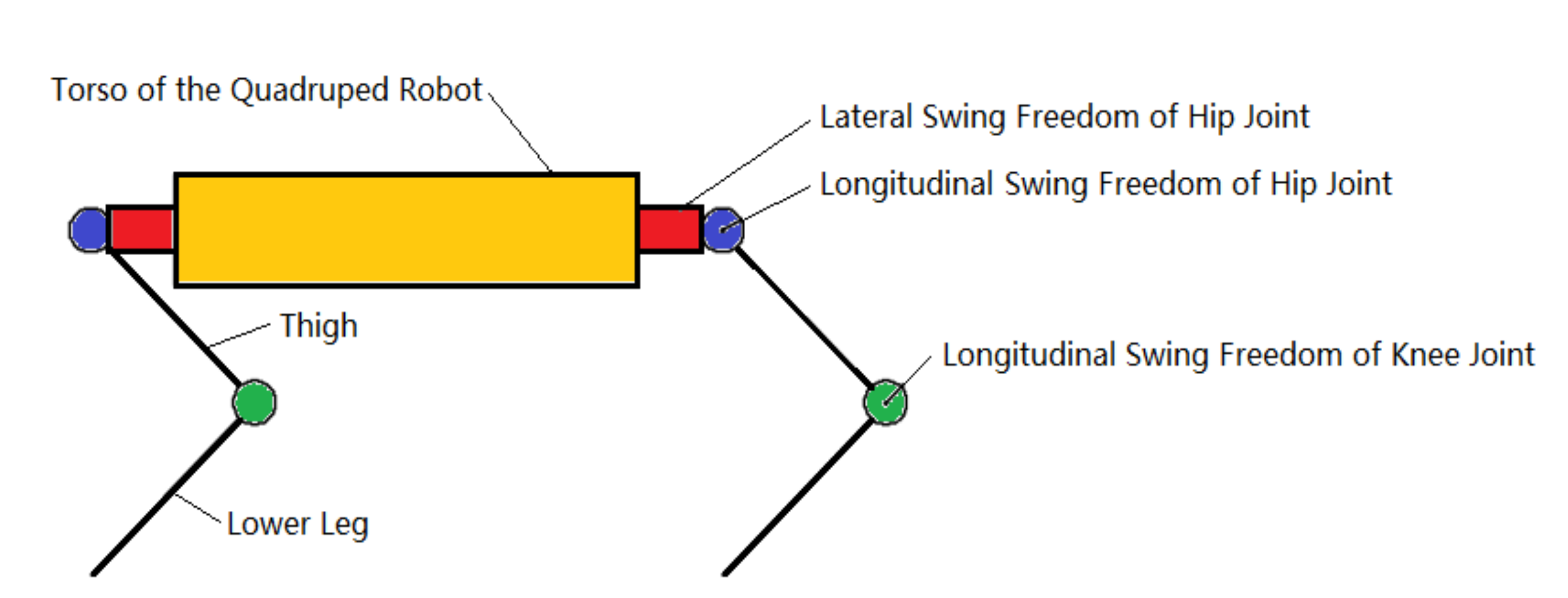
2.1. Topological Structure of the Quadruped Robot

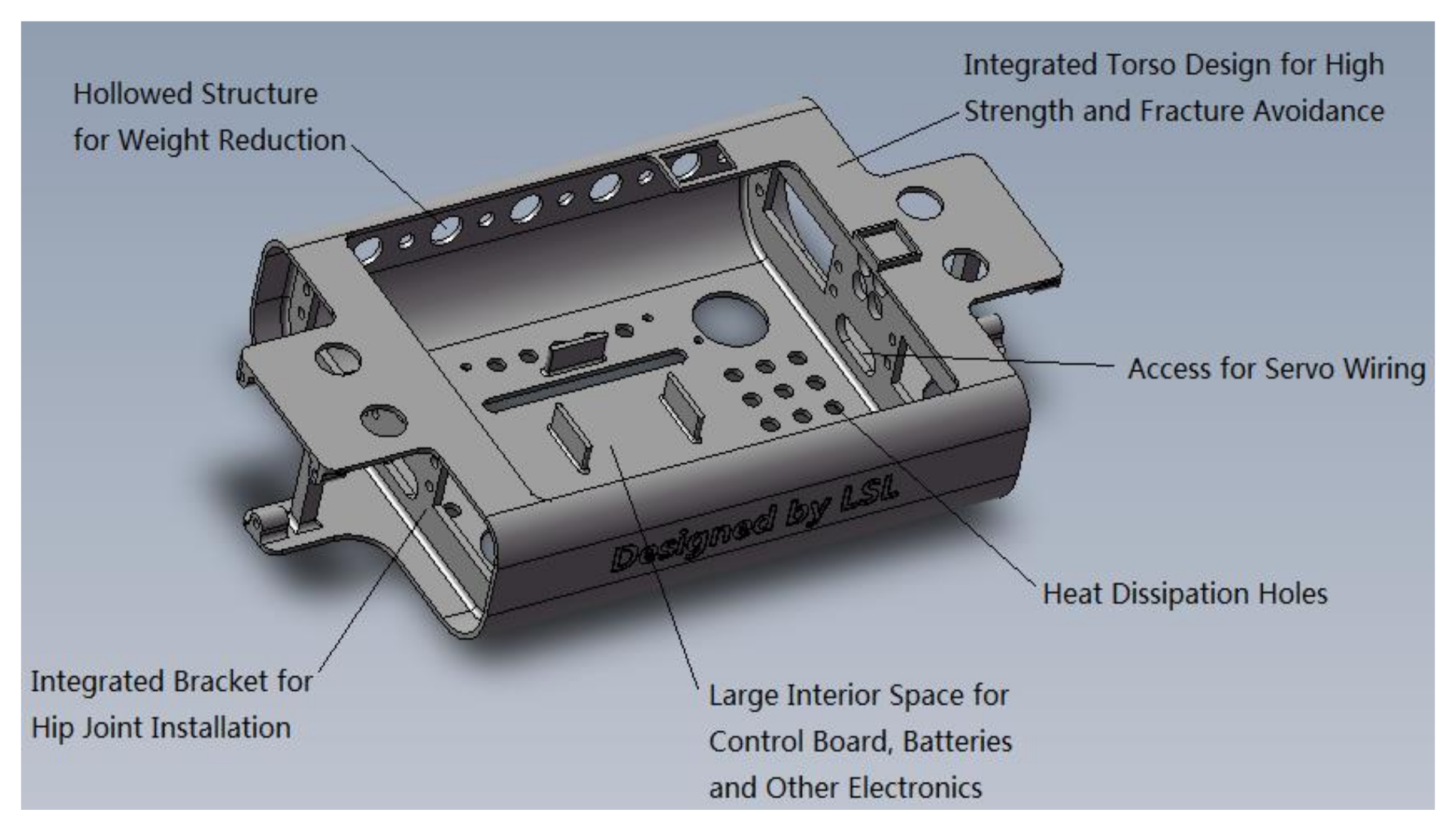
While there is a variety of topology forms for quadruped robot design, the 8, 12 or 16 degrees of freedom (DOF) designs are commonly used. The 8-DOF structure contains four hip joints and four knee joints, with all joint axis parallel to each other. The 8-DOF robot can move forwards or backwards very fast and is relatively easy to control, without the transverse swing freedom of the hip joint. However, the 8-DOF quadruped robot cannot achieve transverse movement and its steering capability is rather limited, leading to poor motion performance. The 16-DOF quadruped robot, on the other hand, has more joints for dexterous locomotion, but it is also more difficult to control. In light of this, the 12-DOF design, with three rotational joints for each leg, is used for our design.

In terms of leg configurations, the inner knee-elbow, outer knee-elbow, full-knee and full-elbow are most popular. The first three leg configurations have a completely symmetrical leg structure, so the robot is more stable, while the last two have more space for movement and are easier to control. Therefore, the full-knee configuration is chosen in this paper. The simplified structural topology is shown below in Figure 1, where the hip joint has both lateral swing and longitudinal swing freedoms, with another swing freedom of the knee joint.

2.2. Torso Design

The torso of the quadruped robot is the central component of the entire robot structure. Four legs are connected together through the torso, so the torso design needs to meet the following requirements. First, sufficient strength is needed to ensure that there will be no deformation, fracture, etc., during the walking process. Next, for dexterous locomotion and energy efficiency, the torso should be designed to be as light as possible. Moreover, there should be sufficient space inside the quadruped robot torso for the installation of servos, batteries, control boards, voltage-converting modules and other components. Finally, the 12 servos mounted on the robot leg joints require a dedicated design and access for wiring, as they are in constant movement, in respect to the torso, when the quadruped robot walks or jogs.

Based on the above requirements, the torso adopts an integrated design, using photosensitive resin with a wall thickness of 2 mm to prevent deformation or fracture. The four corners of the torso are designed to interface with the hip-joint assembly, so that no mechanical interference occurs as the hip joint rotates in any direction. In addition, appropriate hollowing is added at the locations with low load-bearing capacities to reduce weight. The 3D model of the quadruped robot torso structure is shown in Figure 2, below.

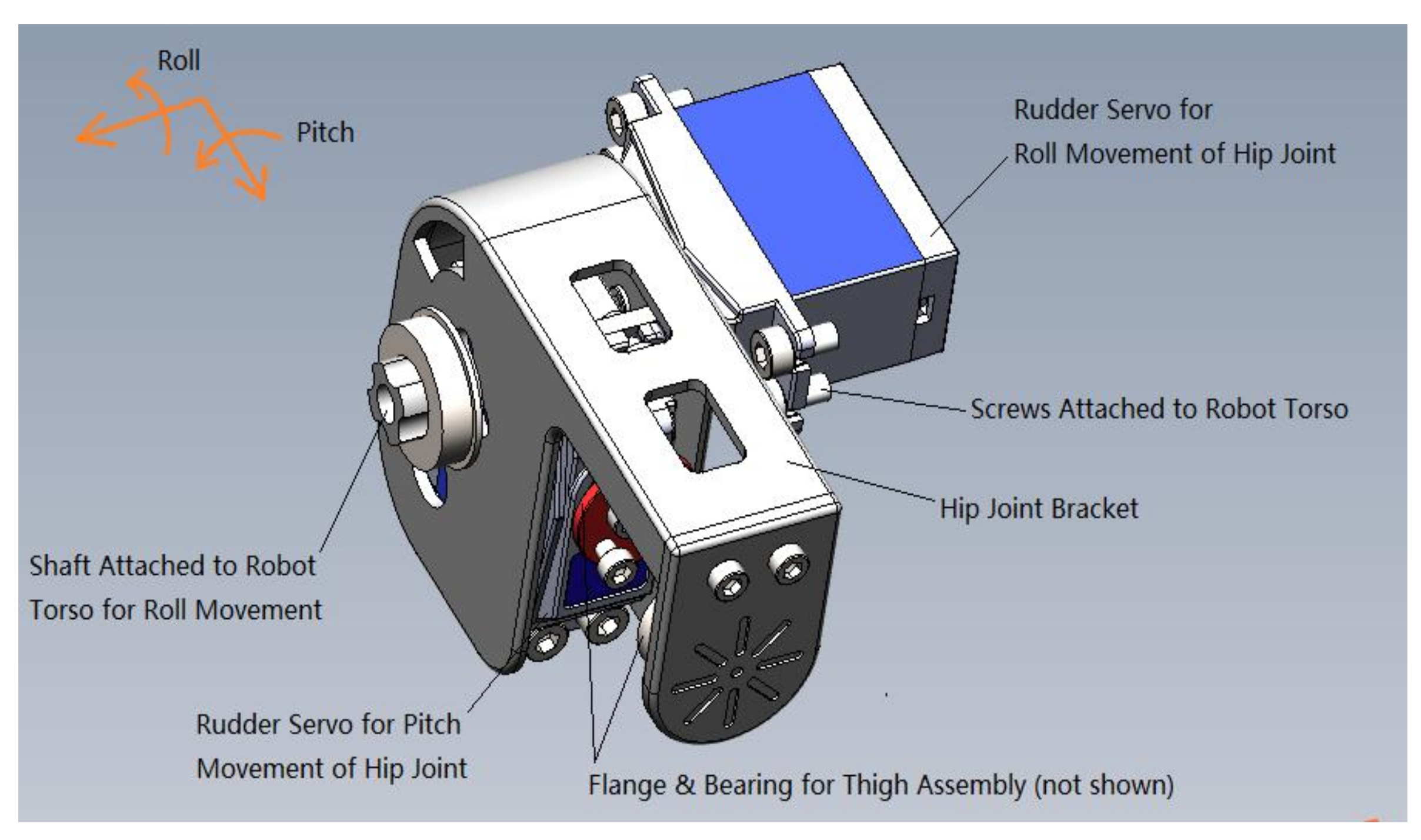
2.3. Hip Joint Design

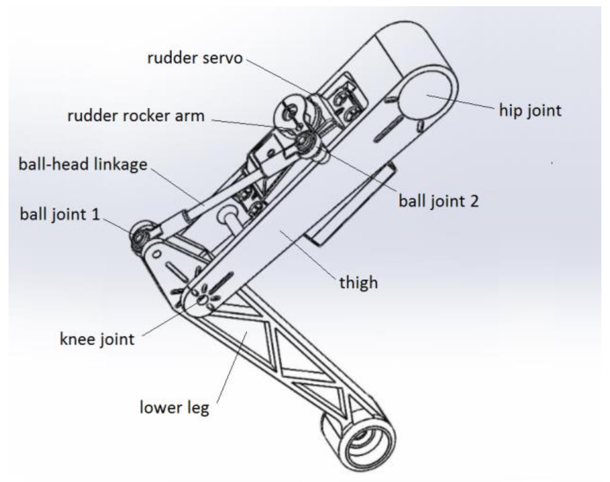
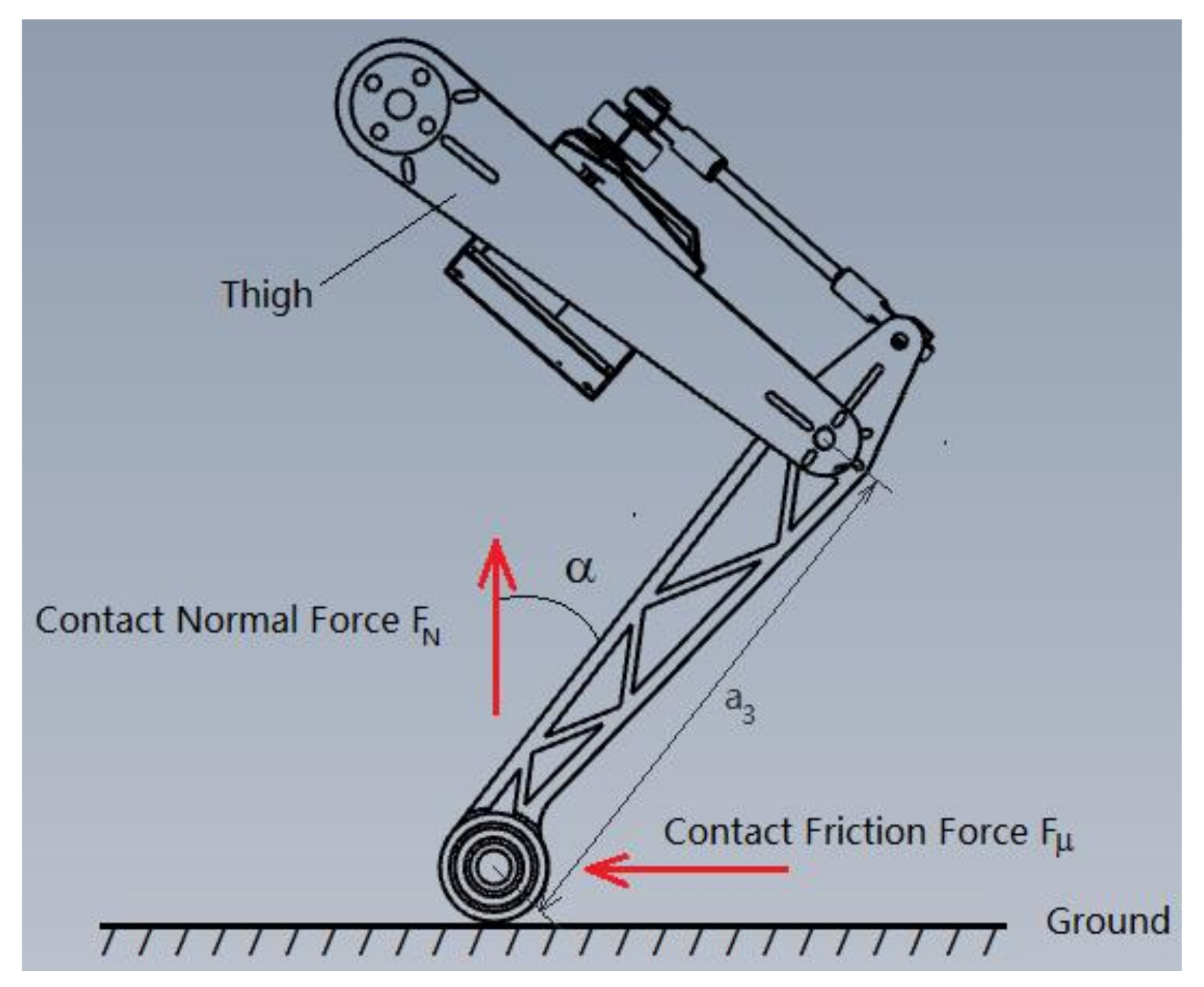
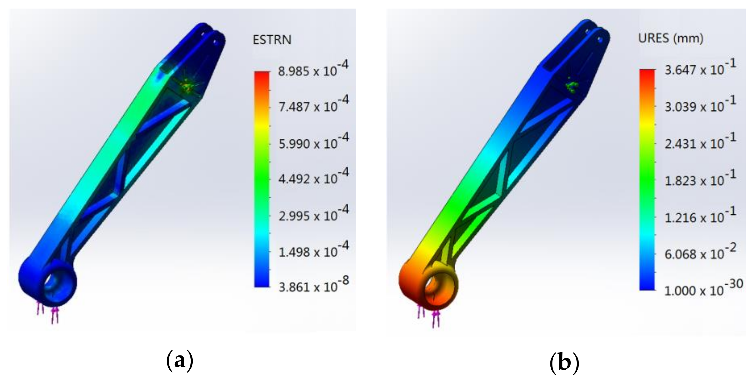
The hip joint of the quadruped robot is designed to generate two degrees of freedom, one for the roll movement and one for the pitch movement. Each movement is actuated by the rudder servo. Since the servo used in our design is a single-axis servo, the F6801zz flange bearings are used on the opposite side of the servo shaft in order to reduce the radial force on it. The shaft end and the hip joint are integrated during fabrication, which facilitates installation and reduces assembly errors. In addition, the servo for the forward swing (i.e., pitch) motion of the hip joint is mounted inside the hip-joint bracket to save space. The 3D model of the hip-joint assembly is shown in Figure 3.

2.4. Leg Design

The legs of the quadruped robot are in frequent contact with the ground as a power source, so leg design is crucial for successful locomotion. The forward swing of the hip joint of the thigh uses bearings to carry axial forces. As the mass of the leg has been ignored in the kinematic calculations presented below, the thigh and lower leg should be designed so that the weight and inertia are as low as possible to reduce theoretical errors. Here, instead of using a direct rudder connection at the knee joint, a ball-head linkage is used with the lower leg being driven indirectly by the rudder rocker arm. This allows for the rudder to be placed on the upper side of the thigh near the hip joint, where the rotational inertia of the leg is relatively low. The single-leg model assembly is shown in Figure 4.

Based on the leg structure of the quadruped robot, it can be seen that the lower leg is most susceptible to fracture and bending as it has to bear the weight of the machine, as well as compact forces, when it touches ground. Here, the ground contact forces are simplified to the normal contact force $F_N$ and tangential contact force $F_{\mu }$ in the vertical plane only, as shown in Figure 5. As the lower leg rotates around the knee-joint axis, ignoring joint friction and contact friction force, the maximum external torque load can be obtained as

$$T_{max}=\eta F_N{a}_3\sin \left(\alpha \right)$$

(1)

where $F_N$ is the normal contact force, a₃ is the length between the knee-joint axis and the ground contact point, $\alpha$ is the angle between the lower leg and the vertical direction and $\eta$ is the dynamic load coefficient. By defining appropriate material properties for each component of the quadruped robot in the SOLIDWORKS model, a total robot weight of approximately $M$ = 2.3 kg is obtained. Assuming the four legs bear the entire weight evenly, the normal contact force F_N is Mg/4 for static situations. Here, a lower leg length of $a_3$ = 0.11 m, a slope angle of $\mathsf{\alpha }$ = 45^°, and a dynamic load coefficient of $\eta$ = 1.2 are used for the numerical strength analysis below.

The load analysis is carried out using the SOLIDWORKS Finite Element Analysis (FEA) simulation plug-in and the strain and displacement diagrams obtained for the lower leg under vertical contact force are shown in Figure 6. Here, the dynamic load coefficient η can always be adjusted (e.g., increased) to account for the influence of the environment, ground–foot contact and the possible movements of the other legs. As can be seen from the results, the strains generated are less than 3.0 × 10⁻⁴ and the maximum displacement under maximum torque is only 0.34 mm, which is in-line with the design requirements.

2.5. Selection of Actuators

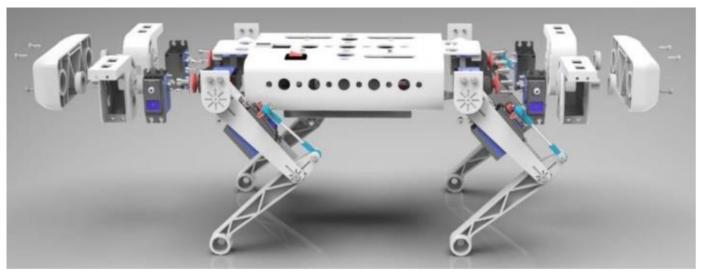
The choice of actuator largely determines the locomotion performance of the quadruped robot. Due to the weight of the robot itself, the actuator has to generate high torque with a fast response and a compact size. Brushless motors are widely used because of their excellent dynamic characteristics, but they are generally less affordable and large in size. Since the main focus of this paper is the implementation and preliminary evaluation of the gait algorithm on the desktop-level model, the rudder servo is selected as the drive source. While the servo does not provide feedback for the angular displacement signal directly, the very high built-in gear ratio of the servo makes it acceptable for low-speed gait and self-balancing tests. The servo model is SPT-5425, as shown in Figure 7, and its specific parameters are shown in

Table 1. Parameters for rudder servo actuator.

Model	Weight	Size (L×W × H)	Operation Voltage	Max Signal Frequency	Range of Rotation	Max Speed	Max Torque
SPT-5425	57 g	40.5 × 20 × 40.5 mm	4.8 V 6 V	330 Hz	10–180°	0.22 s/60° (@4.8 V) 0.18 s/60° (@6 V)	24 kg·cm (@4.8 V) 26 kg·cm(@6 V)

.

To verify the torque rating of the chosen rudder servo, the following analysis is performed. Based on the analysis in Section 2.4, influence of the torque on the lower leg is most significant. Denote the angle between the normal ground contact force $F_N$ and $L_{AB}$ as $\alpha$, and the angle between $L_{DC}$ and $L_{EC}$ (i.e., the length of the ball-head linkage) as $\beta$, shown in Figure 8. Then, the following holds:

$$F_N{L}_{AB}\mathit{sin}\left(\alpha \right)={F^{\prime }}_t{L}_{CB}$$

(2)

where ${F^{\prime }}_t$ is the projection of the ball-head linkage force $F_t$ on $L_{DC}$, namely,

$${F^{\prime }}_t=F_{t}cos\left(\beta \right)$$

(3)

For the given linkage force, when DE is perpendicular to CE, the torque on the servo shaft reaches the maximum, which is calculated by:

$$T_{max}=F{\prime }_t{L}_{DE}$$

(4)

During the low-speed trot gait, there are always two feet contacting the ground as support. Therefore,

$$F_{Nmax}=Mg/2$$

(5)

where $M$ is the total mass of the quadruped robot and $g$ is the gravitational constant.

Substituting Equations (2), (3) and (5) for Equation (4) and considering the dynamic impact contact with the ground yields:

$$T_{max}=\eta Mg{L}_{AB}{L}_{DE}sin\left(\alpha \right)/\left(2L_{CB}\right)$$

(6)

where $\eta$ (>1) is the dynamic load coefficient. By plugging in $M$ = 2.3 kg, $L_{AB}$ = 0.11 m, $L_{DE}$ = 0.024 m, $L_{CB}$ = 0.025 m, $\eta$ = 1.2, $\alpha$ = 45° and $g$ = 9.8 m/s² into the right hand side of Equation (6), $T_{max}$ is found to be 1.01 N·m or 10.3 kg·cm, which is below the rating of the chosen servo (SPT-5425).

2.6. Overall Design

The overall design of the quadruped robot is shown in Figure 9, with a total of 12 degrees of freedom and a full-elbow leg arrangement. Here, all four legs are identical in structure and size for ease of control. The hip joint is directly connected to the rudder in both degrees of freedom to simplify the internal structure, while the knee joint is designed with a rudder rocker plus a linkage to reduce the inertia of the leg. The key parameters are shown in

Table 2. Major parameters of the quadruped robot.

Length	Width	Height	Foot Distance	Thigh Length	Calf Length	Freedom
390 mm	230 mm	180 mm	190 mm	110 mm	110 mm	12

.

3. Forward and Inverse Kinematic Solving

The objective of the robot’s forward kinematics problem is to find the positional representation of the end-effects. In this paper, the most widely used DH coordinate transformation method is explored to solve this problem.

3.1. Establishment of the DH Coordinate System

According to the establishment of the DH coordinate system, the coordinate system $O_b$ is defined as the global coordinate system, which is fixed to the ground. The body coordinate system $O_b$ is located at the geometric center of the torso section of the robot, where $x_b$ is the forward direction of the robot and $z_b$ is the inverse direction of gravitational acceleration. The coordinate systems $O_{k1}$, $O_{k2}$, $O_{k3}$ and $O_{k4}$ (k = 1, 2, 3, 4, respectively) are located at the three rotational joints of each of the four legs and at the ends of the feet. To simplify subsequent calculations, the coordinate system orientations are defined identically for all four legs, with only the positive and negative signs of individual parameters differing. The specific coordinate system orientations are shown in Figure 10.

In the DH method, each linkage can be described by four linkage parameters. When the linkage coordinate system {i} is shown in Figure 4, each linkage parameter is found by the following definition:

• $a_i$ = the distance from $Z_i$ to $Z_{i+1}$ along the $X_i$ axis;
• ${\alpha }_i$ = the angle of rotation around the $X_i$ axis, from $Z_i$ to $Z_{i+1}$;
• $d_i$ = the distance along the $Z_i$ axis, from $X_{i-1}$ to $X_i$;
• ${\theta }_i$ = the angle of rotation around the $Z_i$ axis, from $X_{i-1}$ to $X_i$.

Therefore, using the right front leg of the quadruped robot as an example, the parameters of each linkage are derived as shown in

Table 3. Single-leg joint parameters for quadruped robots.

Linkage	$\mathbf{Linkage}\mathbf{Length}{\mathit{a}}_{\mathbf{i}-1}$		$\mathbf{Linkage}\mathbf{Torsion}\mathbf{Angle}{\mathit{\alpha }}_{\mathbf{i}-1}$	$\mathbf{Linkage}\mathbf{Offset}{\mathit{d}}_{\mathit{i}}$	$\mathbf{Joint}\mathbf{Angle}{\mathit{\theta }}_{\mathit{i}}$
	${\mathit{a}}_{\mathbf{i}-1}$	Value			${\mathit{\theta }}_{\mathit{i}}$	Value
1	0	0	0	0	${\theta }_1$	0
2	0	0	0	$a_1$	${\theta }_2$	90°
3	$a_2$	110	−90°	0	${\theta }_3$	−90°
4	$a_3$	113	0	0	0	/

.

3.2. Forward Kinematics Solving

When solving the forward kinematic equations by the DH method, they are usually decomposed into n sub-problems. The transformation of the linkage coordinate system {i− 1} to the coordinate system {i} creates a coordinate transformation matrix relating only the four linkage parameters ${}_i{}^{i-1}T$. Based on the above definition of each linkage parameter, it follows that:

$${}_i{}^{i-1}T=Tran{s}_x\left\{a_{i-1}\right\}Ro{t}_x\left\{{\alpha }_{i-1}\right\}Tran{s}_z\left\{d_i\right\}Ro{t}_z\left\{{\theta }_i\right\}$$

(7)

Using the right front leg as an example, we have:

$${}_4{}^{0}T=\left[\begin{array}{cccc}c{\theta }_{1}c\left({\theta }_2+{\theta }_3\right)& -c{\theta }_{1}s\left({\theta }_2+{\theta }_3\right)& -s{\theta }_1& a_{2}c{\theta }_{1}c{\theta }_2-a_{1}s{\theta }_1+a_{3}c{\theta }_{1}c\left({\theta }_2+{\theta }_3\right)\\ s{\theta }_{1}c\left({\theta }_2+{\theta }_3\right)& s{\theta }_{1}s\left({\theta }_2+{\theta }_3\right)& c{\theta }_1& a_{1}c{\theta }_1-a_{2}s{\theta }_{1}c{\theta }_2+a_{3}s{\theta }_{1}c\left({\theta }_2+{\theta }_3\right)\\ -s\left({\theta }_2+{\theta }_3\right)& -c\left({\theta }_2+{\theta }_3\right)& 0& -a_{3}s\left({\theta }_2+{\theta }_3\right)-a_{2}s{\theta }_2\\ 0& 0& 0& 1\end{array}\right]$$

(8)

According to Figure 4, the transformation matrix of the coordinate system {$O_{20}$} for {$O_b$} is:

$${}_{20}{}^{b}T=\left[\begin{array}{cccc}0& 0& 1& b\\ 0& 1& 0& -w\\ -1& 0& 0& 0\\ 0& 0& 0& 1\end{array}\right]$$

(9)

Thus, the transformation matrix of the foot-end coordinate system {$O_{24}$} of the right forefoot relative to {$O_b$} is found to be:

$${}_{24}{}^{b}T={}_{20}{}^{b}T{}_4{}^{0}T=\left[\begin{array}{cccc}-s\left({\theta }_2+{\theta }_3\right)& -c\left({\theta }_2+{\theta }_3\right)& 0& b-a_{3}s\left({\theta }_2+{\theta }_3\right)-a_{2}s{\theta }_2\\ s{\theta }_{1}c\left({\theta }_2+{\theta }_3\right)& -s{\theta }_{1}s\left({\theta }_2+{\theta }_3\right)& c{\theta }_1& a_{1}c{\theta }_1+a_{2}s{\theta }_{1}c{\theta }_2+a_{3}s{\theta }_{1}c\left({\theta }_2+{\theta }_3\right)-w\\ -c{\theta }_{1}c\left({\theta }_2+{\theta }_3\right)& c{\theta }_{1}s\left({\theta }_2+{\theta }_3\right)& s{\theta }_1& a_{1}s{\theta }_1-a_{3}c{\theta }_{1}c\left({\theta }_2+{\theta }_3\right)-a_{2}c{\theta }_{1}c{\theta }_2\\ 0& 0& 0& 1\end{array}\right]$$

(10)

This gives the forward kinematic equation for the right front leg.

3.3. Inverse Kinematic Solving

According to:

$${}_4{}^{0}T={}_1{}^{0}T{}_2{}^{1}T{}_3{}^{2}T{}_4{}^{3}T$$

(11)

After simplification, one can get the equations:

$$\left\{\begin{array}{c}\left(x_{0}c{\theta }_1+y_{0}s{\theta }_1\right)c{\theta }_2-z_{0}s{\theta }_2=a_2+a_{3}c{\theta }_3\\ -\left(x_{0}c{\theta }_1+y_{0}s{\theta }_1\right)s{\theta }_2-z_{0}c{\theta }_2=a_{3}s{\theta }_3\\ y_{0}c{\theta }_1-x_{0}s{\theta }_1-a_1=0\end{array}\right.$$

(12)

The solutions are:

$$\left\{\begin{array}{c}{\theta }_1={\mathit{sin}}^{-1}(-\frac{a_1}{\sqrt{x_0^2+y_0^2}})+\varphi \\ {\theta }_2=\pm {\mathit{sin}}^{-1}(\frac{-a_{3}s{\theta }_3}{\sqrt{{(x_{0}c{\theta }_1+y_{0}s{\theta }_1)}^2+z_0^2}}-\alpha )\\ {\theta }_3=\pm {\mathit{cos}}^{-1}(\frac{\left(x_{0}c{\theta }_1+y_{0}s{\theta }_1\right)+z_0^2-a_2^2-a_3^2}{2a_2{a}_3})\end{array}\right.$$

(13)

The above equations are the solutions to the system of inverse kinematic equations for the right front leg, where ${\theta }_2$ is taken as positive and ${\theta }_3$ as negative drawn.

4. Gait Planning and Motion Analysis

Gait planning is central to the stable movement of quadruped robots. In nature, quadruped mammals choose different gaits depending on the desired speed of movement and the ruggedness of the land surface to minimize their energy consumption while achieving their desired movement. On this basis, the common gait patterns of animals have been extracted to provide a basis for gait planning in quadruped robots.

4.1. Common Gait Patterns for Quadruped Robots

Currently, the five most commonly used gaits are the walk, trot, pace, bound and gallop gait. The trot gait is the most common. It is a typical “two-beat” gait, where the two diagonal legs have identical movement characteristics, with the left front leg and right rear leg in unison and the right front leg and left rear leg in unison, as shown in Figure 11. Theoretically, the duty cycle coefficient in this gait is not subject to any restriction, and 0 <β< 1. Thus, the robot has a wide range of speeds and can choose different speeds for different terrains. In addition, some scholars have conducted experiments on the amount of oxygen consumed by horses in different gaits (walk, trot and gallop) using different movement speeds [37], and studies show that the trot gait is relatively low in oxygen consumption over a relatively large range of speeds, which also suggests that this gait has theoretically high energy efficiency [38,39].

Depending on the value of the duty cycle factor, the diagonal trot gait can be divided into three types. When β < 0.5, the robot has a brief vacant phase (the moment when all four legs are in the swing phase) and the speed of movement increases significantly, but the presence of the vacant phase also greatly increases the difficulty of control. When β > 0.5, the robot has four sets of supports when the swing leg switches, which ensures stability but reduces the speed of movement. When β = 0.5, two sets of diagonal legs switch seamlessly between the oscillating and supporting phases, which is somewhere in between; it also provides a balance between speed and robot stability, making it the dominant gait choice.

4.2. Footpath Planning

Once the main gait of the robot has been determined, the individual foot-end trajectories need to be planned to achieve the robot’s motion. The most common method of foot-trajectory planning is to give separate foot trajectory functions for the swing and support feet, and to link them together to form a closed-loop trajectory within a gait cycle. The key to this control method is the state of the foot end at the moment of contact with the ground. The stability of the robot body is determined to a large extent by the contact and friction forces on the foot end when it touches the ground. With these objectives in mind, it is possible to design a variety of foot trajectories.

The most widely used of these should be the composite cycloid function, using the transverse pendulum coordinate system of each leg as the base coordinate system. Setting ($x_0,y_0,z_0$) as the swing foot starting coordinates, ($x_f,y_f,z_f$) are the coordinates of the desired landing point. The equation of the trajectory is shown below:

$$\left\{\begin{array}{c}{x}_{sw}=\left(x_f-x_0\right)\frac{\left(\varphi -\sin \varphi \right)}{2\pi }+x_0\\ y_{sw}=\left(y_f-y_0\right)\frac{\left(\varphi -\sin \varphi \right)}{2\pi }+y_0\\ z_{sw}=\Delta h_d\frac{\left(1-\cos \varphi \right)}{2\pi }+z_0\end{array}\right.$$

(14)

Here, $\varphi =\frac{2\pi t}{T_{sw}}$, $\Delta h_d$ is the desired lift height of the swing leg and $T_{sw}$ is the swing phase time within a gait cycle. Since the chosen diagonal trot gait duty cycle factor is β = 0.5, $T_{sw}$ = 0.5T. t is the time differentiation and 0 ≤ t ≤ $T_{sw}$.

For the desired landing point coordinates ($x_f,y_f,z_f$), which are not available for the real-time velocity of the robot, they are simply set to:

$$\left\{\begin{array}{c}{x}_f=\frac{1}{2}{\dot{x}}_d{T}_{st}\\ y_f=\frac{1}{2}{\dot{y}}_d{T}_{st}\\ z_f=z_0\end{array}\right.$$

(15)

where T_st is the support phase time within a gait cycle and ${\dot{x}}_d$ and ${\dot{y}}_d$ are the desired velocities of motion in the x and y directions, respectively. The step length of each step increases as the desired velocity of motion increases. In this paper, ($x_0,y_0,z_0$) = (0, 0, 0), ($x_f,y_f,z_f$) = (10, 0, 0), $\mathsf{\Delta }{h}_d$ = 5 cm and $T_{sw}$ = 1 s are used.

5. Dynamics and Simulation Based on ADAMS and MATLAB

In this paper, the dynamic model of the quadruped robot is formulated using the Newton–Euler methods, with the consideration of foot–ground contact. The dynamics of a quadruped robot are then simulated using a combination of ADAMS and MATLAB. The virtual prototype model is first built in SOLIDWORKS and imported into ADAMS to add various constraints, contact forces, friction and other parameters. The Simulink module in MATLAB is used to complete the design and simulation of the control system. The simulation results are then analyzed and compared.

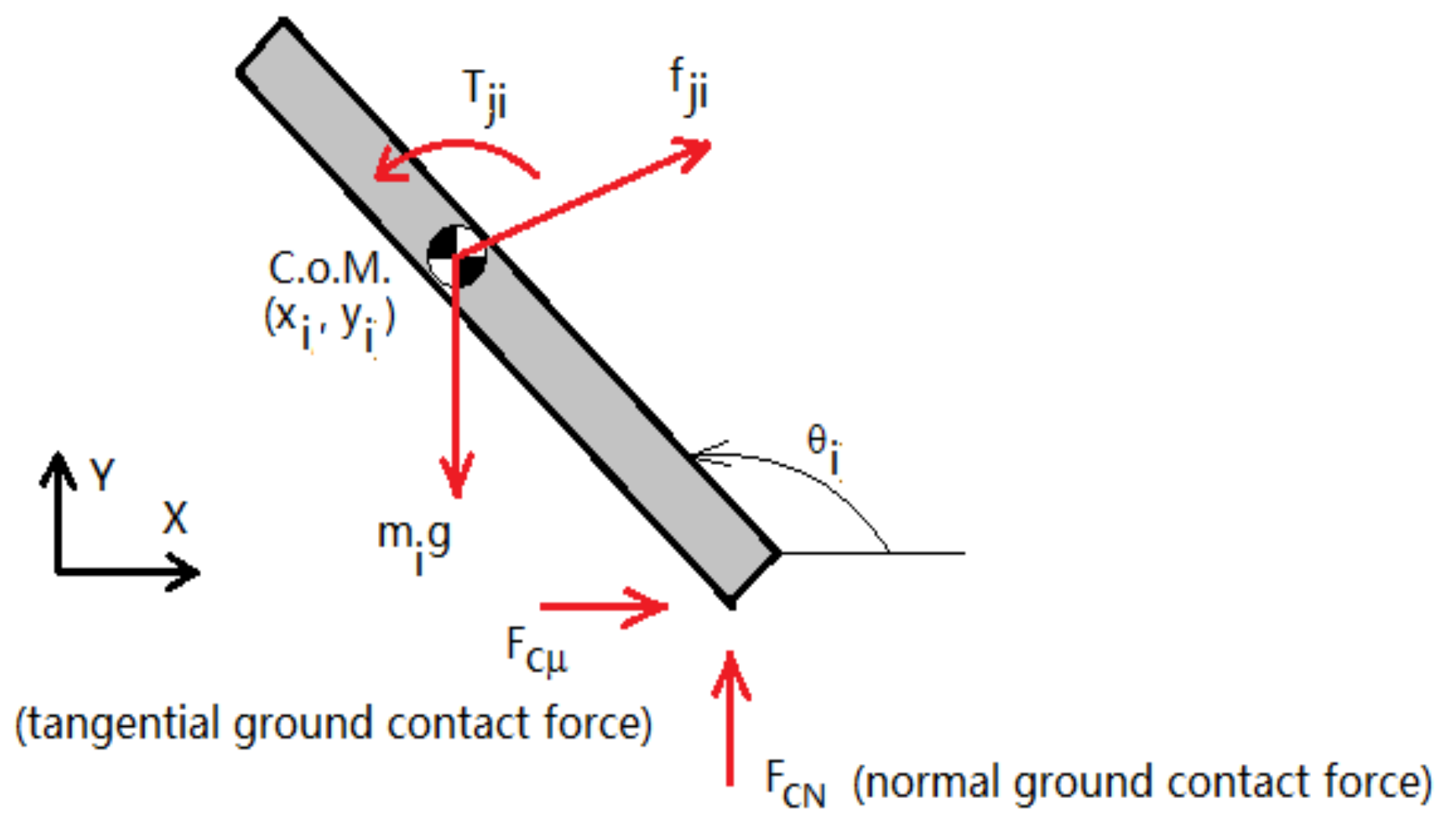
5.1. Dynamic Modeling

When the quadruped robot is in operation, forces and torques from adjacent links and/or the ground act on each individual link i, as shown in Figure 12. Using the Newton–Euler method, for any general link i of the quadruped robot, the dynamic equations for the motion of its center of mass (C.o.M.) and for the rotation of the rigid body can be written as [35]

$$\left\{\begin{array}{c}{\displaystyle {\displaystyle \sum }_i}{F}_i=m_i{a}_i\\ f_{ij}=-f_{ji}\\ {\displaystyle {\displaystyle \sum }_i}{T}_i=I_i{\ddot{\theta }}_i\end{array}\right.$$

(16)

Equation (16) can be further written in joint space [40], namely,

$$M\left(q\right)\ddot{q}+C\left(q,\dot{q}\right)\dot{q}+G\left(q\right)=F_S-J^T\left(q\right)F_C$$

(17)

where $M\left(q\right)$ is the generalized inertial matrix, $C\left(q,\dot{q}\right)$ is the Coriolis and centrifugal force vector, $G\left(q\right)$ is the gravity vector, $F_S$ is the force vector of joint servos and $J^T\left(q\right)$ is the Jacobian matrix for the lower legs. Here, $F_C$ is the ground contact force vector and is calculated by the Ristow model [35]:

$$F_{CN}=K{\delta }^{1.5}+\chi m_{eff}\dot{\delta }$$

(18)

where $K$ is the stiffness coefficient, $\delta$ is the indentation of contact, $m_{eff}$ is the equivalent mass of two bodies of contact and $\chi$ is the correction factor based on experimental results.

5.2. Virtual Prototyping

The creation of the virtual prototype model is done in the 3D modeling software SOLIDWORKS. To improve the efficiency of the simulation in ADAMS, the 3D model is idealized as follows:

(1)

Deletion of parts that are not relevant to the simulation, such as control plates, bolts, nuts, etc.;

(2)

Appropriate reduction of part features, such as rounded corners, chamfers, hollowing, etc.;

(3)

Reducing the number of parts in the assembly by combining parts that can be considered as a whole into a single part using Boolean operations.

After the above operations, the final model consists of only 13 parts: the body, the hip joints of the four legs, the thighs and the lower legs. The model was then imported into ADAMS and the virtual prototype model in ADAMS is shown in Figure 13. The initial angles of the joints are: ${\theta }_1$ = 0°, ${\theta }_2$ = 45° and ${\theta }_3$ = −90°.

5.3. ADAMS and MATLAB Simulation

The control system, designed using the Simulink toolbox in MATLAB, consists of two major sub-modules:

(1)

The gait function generates foot-end trajectory functions for the swing and support phases in a single cycle;

(2)

The inverse-kinematics function converts the pre-planned foot-end trajectory function into a function of the joint angles using the inverse kinematic solution.

The simulation time is T_sim = 30 s, the gait period is 0.5 s, the swing leg lift height is 10 mm and the distance travelled in one gait period is 70 mm.The joint curves are then imported into ADAMS to create spline curves as joint drivers.

To investigate the performance of the quadruped robot in rough terrain, the ground shape was set as shown in Figure 14. The entire simulation was divided into 3 stages: (1) planar advance, (2) up a 5° slope, and (3) down a 5° slope. For a successful simulation of the quadruped robot jogging on the terrain, proper contact modeling between the feet and ground is crucial for minimizing foot–ground slippage and ensuring numerical convergence. Here, the impact-function-based contact model is used in ADAMS, and the detailed contact model parameters are shown in

Table 4. Parameters for foot–ground contact model.

Normal Force	Stiffness	Force Exponential	Damping	Penetration Depth	Friction	Static Coefficient	Dynamic Coefficient	Friction Transition Velocity	Stiction Transition Velocity
Impact	2855 N/m	1.1	10 N·s/mm	0.57 mm	Coulomb	0.8	0.75	0.1	10

. More details and in-depth analyses on modeling foot–ground contact with slippage can be found in [35,36]. The simulation was then carried out with a simulation time of T_s = 25 s and a simulation step size of 0.07 s.

5.4. Analysis of Simulation Results

As can be seen from Figure 15, the pitch angle fluctuates within a gait cycle of around 3° on level ground. The mean value of the pitch angle varies with the terrain during the ascent and descent, with the difference between the maximum and minimum values being around 10°. According to Figure 16, the value of the roll angle also varies during a gait cycle, remaining largely within 6°. The variation in gait angle is a general indication of the stability of the robot’s motion, and the algorithm will continue to be optimized in subsequent work to reduce the range of gait angle fluctuations.

6. Physical Design and Experimental Validation

6.1. Description of the Prototype

After completing the above, a prototype was designed, fabricated and commissioned. The prototype has 12 degrees of freedom and uses the SCS0009 bus servo as the drive for each joint. To reduce the complexity and weight of the mechanism, the servo is fixed in a direct connection to each joint and a miniature bearing is added to the other side of the servo output shaft to improve the radial force capacity on the servo shaft. The entire robot is 3D printed and made from PLA, with a total weight of 1.2 kg.

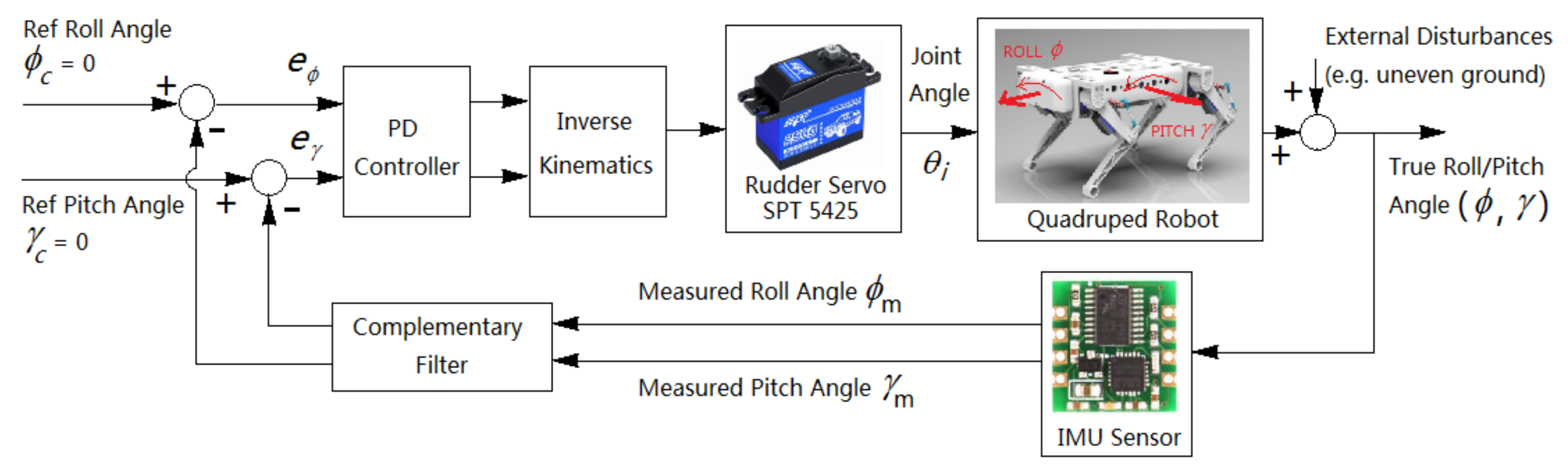
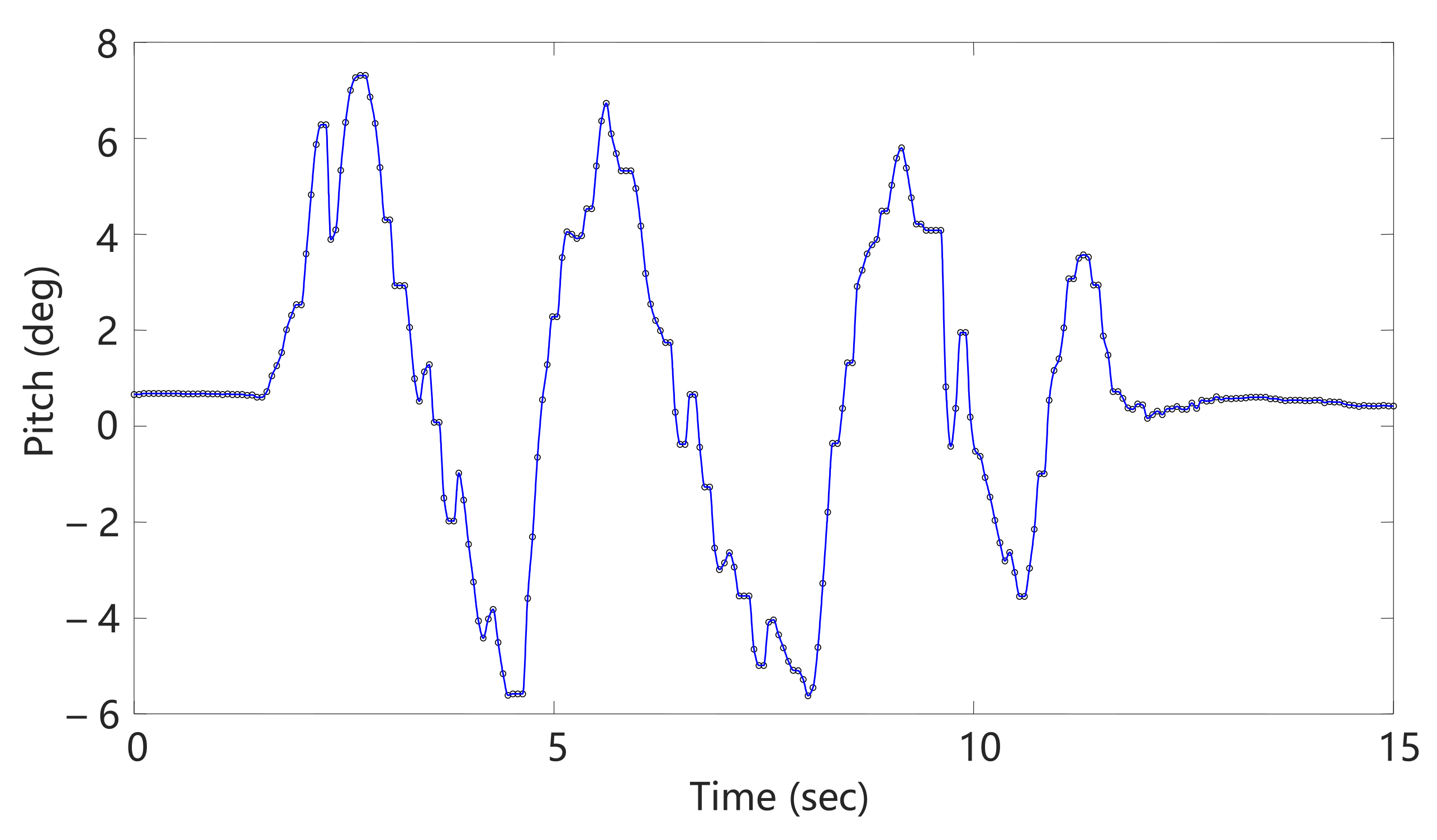
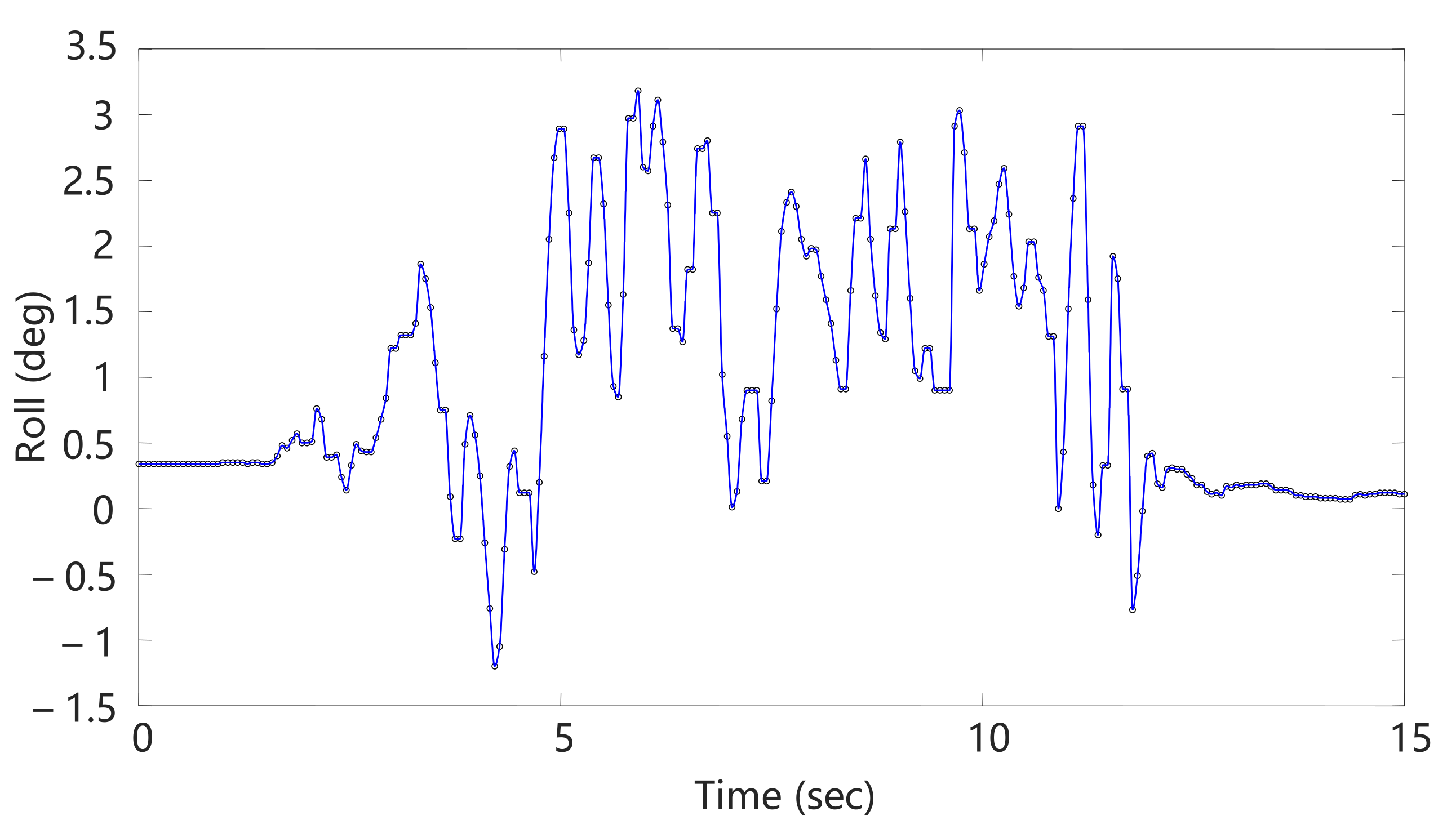
6.2. Diagonal Trot Gait Experiment

To investigate the fluctuation of the body during the movement, the gyroscope module inside the body was used to obtain the attitude angle data and plot the pitch and roll angles, respectively. The pitch and roll curves are shown in Figure 17 and Figure 18. The angles fluctuate regularly within a specific range, where the fluctuation range of the pitch angle is around 7° and the roll angle around 10°, with a large disturbance at the moment of start and stop of the robot’s trot motion.

As the quadruped robot performs the trot gait, it has to maintain self-balance. Figure 19 shows the block diagram of the self-balancing controller of the quadruped robot. When the ground underneath is uneven or tilts, it causes the quadruped robot to tilt. The roll and pitch angles (φ, γ) are measured by the gyroscope and accelerometer modules on the IMU sensor board, which are further processed by using the complementary filter. The filtered roll and pitch angles are then compared with the reference/desired roll and pitch, both of which are 0 for the self-balancing purpose. Here, an elementary yet effective PD controller is used to process error signals from the roll and pitch. The inverse kinematics solver further converts the results to joint angle rudder servos (SPT 5425), which subsequently adjusts the length of each leg of the quadruped robot. The feedback control loop is fighting to bring both the quadruped robot’s roll and pitch angles to zero whenever the body of the quadruped robot tilts in real time, so that the quadruped robot maintains self-balance.

To verify the self-balancing capability of the robot, it was placed on a freely rotating disc (Figure 20) and the Euler angular variation output from the gyroscope was extracted as the disc angle was continuously changed, as shown in Figure 21 and Figure 22. It can be seen that the robot can adjust its attitude by adjusting the support height of the four legs as the body tilts due to the tilting of the support surface of the disc, with the pitch angle fluctuating between +7° and 5° and the roll angle fluctuating between +3° and −1.2°. Due to the hardware limitations of the gyroscope and the speed of the servo, the response time of the quadruped robot to external disturbances is not very fast and the robot’s attitude angles can sometimes be over-adjusted.

7. Conclusions

This paper focuses on the structural design, kinematic modeling, gait planning, dynamics simulation, physical fabrication and experimental verification of a quadruped robot. The Ristow model is used to characterize the nonlinear dynamic phenomenon of foot–ground contact. A composite cycloidal foot trajectory equation is developed to reduce the ground impact at the moment of touchdown to a certain extent, which is beneficial to the stability of the robot. A physical model of the quadruped robot is designed and implemented. STM32 microcontroller is chosen as the controller and a FreeRTOS system is used as the control framework. In the diagonal trot gait experiment and self-balancing test, the quadruped robot is able to control the roll and pitch angles of its torso. A certain amount of slippage is observed between the robot foot and the ground, which limits the quadruped robot’s locomotive speed. Possible causes include inadequate modeling and control of the foot–ground contact and interaction, as well as the use of hobby servos without feedback, which will be the focus of our future research. The design of this work provides an affordable yet comprehensive platform for novice researchers in the field to study the complex problems of dynamics, contact modeling, gait planning and attitude control for quadruped robots.

References

1. Zhang, F.; Teng, S.; Wang, Y. Design of Bionic Goat Quadruped Robot Mechanism and Walking Gait Planning. Int. J. Agric. Biol. Eng. 2020, 13, 32–39. [Google Scholar] [CrossRef]
2. Rajat, K.; Kanaiya, G.; Nikhil, K. Overview of Different Techniques Utilized in Designing of a Legged Robot. Glob. J. Enterp. Inf. Syst. 2017, 9, 1–6. [Google Scholar]
3. Priyaranjan, B.; Mohanty, K. Development of Quadruped Walking Robots: A Review. Ain Shams Eng. J. 2021, 12, 2017–2031. [Google Scholar]
4. Zhang, S.; Fan, M.; Li, Y. Generation of a Continuous Free Gait for Quadruped Robot over Rough Terrains. Adv. Robot. 2019, 33, 74–89. [Google Scholar] [CrossRef]
5. Meng, X.; Wang, S.; Cao, Z. A Review of Quadruped Robots and Environment Perception. In Proceedings of the 35th Chinese Control Conference (CCC), Chengdu, China, 27–29 July 2016; pp. 6350–6356. [Google Scholar]
6. Liu, H.; Zhang, X.; Fu, C.; Ma, H. Compliant Gait Generation for a Quadruped Bionic Robot Walking on Rough Terrains. Robot 2014, 36, 584–591. [Google Scholar]
7. Srinivas, T. Valkyrie—Design and Development of Gaits for Quadruped Robot Using Particle Swarm Optimization. Appl. Sci. 2021, 11, 7458. [Google Scholar] [CrossRef]
8. Raza, F. Balance Stability Augmentation for Wheel-Legged Biped Robot through Arm Acceleration Control. IEEE Access 2021, 9, 54022–54031. [Google Scholar] [CrossRef]
9. Kim, J. Design and Control of a Open-Source, Low Cost, 3D Printed Dynamic Quadruped Robot. Appl. Sci. 2021, 11, 3762. [Google Scholar] [CrossRef]
10. Li, Y.; Li, B.; Ruan, J.; Rong, X. Research of Mammal Bionic Quadruped Robots: A Review. In Proceedings of the 5th International Conference on Robotics, Automation and Mechatronics (RAM), Qingdao, China, 17–19 September 2011; pp. 166–171. [Google Scholar]
11. Xing, B.; Feng, P.; Feng, X. Improved ZMP Crawling Gait Algorithm for Quadruped Robot Based on Intelligent Decision Making. Comput. Eng. Appl. 2019, 55, 206–257. [Google Scholar]
12. Min, I.; Yoo, D.; Min, S. Body Trajectory Generation Using Quadratic Programming in Bipedal Robots. In Proceedings of the 20th International Conference on Control, Automation and Systems (ICCAS), Busan, Korea, 13–16 October 2020; pp. 251–257. [Google Scholar]
13. Han, B.; Wang, Q.; Jia, Y. Trot Gait Planning Method for Improving the Stability of Quadruped Robot. Beijing LigongDaxueXuebao/Trans. Beijing Inst. Technol. 2018, 38, 917–920. [Google Scholar]
14. Gianluca, P. Maicol and Belfiore. Quadrupedal Robots’ Gaits Identification via Contact Forces Optimization. Appl. Sci. 2021, 11, 2102. [Google Scholar]
15. Liu, Y.; Zhou, C.; Guo, J. Single-Step Emergency Stop Stability Control Strategy for Quadruped Robot. J. Nanjing Univ. Sci. Technol. 2020, 44, 259–265. [Google Scholar]
16. Xu, J.; Ge, L.; Wang, J. ZMP Preview Control Based Compliance Control for a Walking Quadruped Robot. In Proceedings of the 2015 IEEE International Conference on Information and Automation, Lijiang, China, 8–10 August 2015; pp. 7–12. [Google Scholar]
17. Zhang, D.; Zheng, W.; Yang, Y. CPG-Based Gait Control Method for Quadruped Robot Jumping Movement. In Proceedings of the 7th International Conference on Control, Automation and Robotics (ICCAR), Singapore, 23–26 April 2021; pp. 41–45. [Google Scholar]
18. Liu, M. Local CPG Self Growing Network Model with Multiple Physical Properties. Appl. Sci. 2020, 10, 5497. [Google Scholar] [CrossRef]
19. Zhang, D.; Zheng, W. Design and Gait Optimization of Quadruped Robot Based on Energy Conservation. In Proceedings of the 3rd International Conference on Control and Robots (ICCR), Tokyo, Japan, 26–29 December 2020; pp. 112–119. [Google Scholar]
20. Shang, L.; Li, Z. Smooth Gait Transition Based on CPG Network for a Quadruped Robot. In Proceedings of the 2019 IEEE/ASME International Conference on Advanced Intelligent Mechatronics (AIM), Hong Kong, China, 8–12 July 2019; pp. 358–363. [Google Scholar]
21. Takahiro, F. Autonomous Gait Transition and Galloping over Unperceived Obstacles of a Quadruped Robot with CPG Modulated by Vestibular Feedback. Robot. Auton. Syst. 2019, 111, 1–19. [Google Scholar]
22. Liu, C.; Chen, Q.; Wang, D. CPG-Inspired Workspace Trajectory Generation and Adaptive Locomotion Control for Quadruped Robots. IEEE Trans. Syst. ManCybern. Part B: Cybern. 2011, 41, 867–880. [Google Scholar]
23. Lu, G.; Chen, T.; Liu, Q. A Novel Multi-Configuration Quadruped Robot with Redundant DOFs and Its Application Scenario Analysis. In Proceedings of the 2021 International Conference on Computer, Control and Robotics (ICCCR), Shanghai, China, 8–10 January 2021; pp. 14–20. [Google Scholar]
24. Gong, D. Bionic Quadruped Robot Dynamic Gait Control Strategy Based on Twenty Degrees of Freedom. IEEE/CAA J. Autom. Sin. 2018, 5, 382–388. [Google Scholar] [CrossRef]
25. Yang, J.; Sun, H.; Wu, D. SLIP Model-Based Foot-to-Ground Contact Sensation via Kalman Filter for Miniaturized Quadruped Robots. In Proceedings of the Intelligent Robotics and Applications: 12th International Conference, ICIRA 2019, Shenyang, China, 8–11 August 2019; p. 3. [Google Scholar]
26. Hiroshi, T.; Masato, D.; Jun, U. Slip-Adaptive Walk of Quadruped Robot. Robot. Auton. Syst. 2005, 53, 124–141. [Google Scholar]
27. Seo, J.; Kim, J. A SLIP-Based Robot Leg for Decoupled Spring-like Behavior: Design and Evaluation. Int. J. Control. Autom. Syst. 2019, 17, 2388–2399. [Google Scholar] [CrossRef]
28. Chen, T.; Rong, X.; Li, Y.; Ding, C. A Compliant Control Method for Robust Trot Motion of Hydraulic Actuated Quadruped Robot. Int. J. Adv. Robot. Syst. 2018, 15, 1729881418813235. [Google Scholar] [CrossRef] [Green Version]
29. Chen, G. Dynamic Balance and Trajectory Tracking Control of Quadruped Robots Based on Virtual Model Control. In Proceedings of the 39th Chinese Control Conference (CCC), Shenyang, China, 27–29 July 2020; pp. 3771–3776. [Google Scholar]
30. Zhao, J. Fractional-Order Virtual Model Control for Trotting Motion of Quadruped Robot. In Proceedings of the Chinese Control And Decision Conference (CCDC) 2020, Hefei, China, 22–24 August 2020; pp. 4935–4942. [Google Scholar]
31. Lin, G.; Jia, W.; Ma, S. Research and Analysis of Comprehensive Optimization Method for Energy Consumption and Trajectory Error of the Leg Structure Based on Virtual Model Control. In Proceedings of the 2021 IEEE International Conference on Mechatronics and Automation (ICMA), Takamatsu, Japan, 8–11 August 2021; pp. 1094–1099. [Google Scholar]
32. Zhang, G. Torso Motion Control and Toe Trajectory Generation of a Trotting Quadruped Robot Based on Virtual Model Control. Adv. Robot. 2016, 30, 284–297. [Google Scholar] [CrossRef]
33. Meng, J. A Dynamic Balancing Approach for a Quadruped Robot Supported by Diagonal Legs. Int. J. Adv. Robot. Syst. 2015, 12, 10. [Google Scholar] [CrossRef] [Green Version]
34. Zhang, Y.; Guo, Z.; Chen, D. Gait Control of Quadruped Robot Driven by Pneumatic Muscle Based on Kimura Oscillator and Virtual Model. Acta Armamentarii 2018, 39, 1411–1418. [Google Scholar]
35. Corral, E.; Moreno, R.G.; García, M.G.; Castejón, C. Nonlinear Phenomena of Contact in Multibody Systems Dynamics: A Review. Nonlinear Dyn. 2021, 104, 1269–1295. [Google Scholar] [CrossRef]
36. Corral, E.; Meneses, J.; Castejon, C.; Garcia-Prada, J. Forward and Inverse Dynamics of the Biped PASIBOT. Int. J. Adv. Robot. Syst. 2014, 11, 109. [Google Scholar] [CrossRef]
37. Hoyt, D.; Taylor, C. Gait and the Energetics of Locomotion in Horses. Nature 1981, 292, 239–240. [Google Scholar] [CrossRef]
38. Lei, J.; Wang, F. Energy Consumption Analysis of Quadruped Robot with Trot Gait. Appl. Mech. Mater. 2013, 271, 1531–1535. [Google Scholar] [CrossRef]
39. Gao, F.; Lei, J.; Xu, G. Trot Gait and Energy Consumption Simulation of a Quadruped Robot. J. Beijing Univ. Aeronaut. Astronaut. 2007, 33, 719–722. [Google Scholar]
40. Chenkun, Q.; Feng, G.; Xianchao, Z.; Qiao, S.; Xinghua, T.; Xianbao, C. Dynamic Model Based Ground Reaction Force Estimation for a Quadruped Robot Without Force Sensor. In Proceedings of the 34th Chinese Control Conference (CCC), Hangzhou, China, 28–30 July 2015; pp. 6084–6089. [Google Scholar]
Figure 1. Structure topology of the 12-DOF quadruped robot design (front view).
Applsci 11 10705 g001
Figure 2. Integrated torso design for high strength and light weight.
Applsci 11 10705 g002
Figure 3. Hip-joint assembly for the lateral and longitudinal swing motions.
Applsci 11 10705 g003
Figure 4. Single leg assembly.
Applsci 11 10705 g004
Figure 5. Force diagram for lower leg tip of the quadruped robot as it contacts ground.
Applsci 11 10705 g005
Figure 6. Load analysis of the lower leg: (a) cloud diagram for strain analysis; (b) cloud diagram for total displacement analysis.
Applsci 11 10705 g006
Figure 7. Servo actuator (model SPT-5425) for quadruped robot.
Applsci 11 10705 g007
Figure 8. Torque analysis of the lower leg servo actuator.
Applsci 11 10705 g008
Figure 9. 3D exploded view of the quadruped robot assembly.
Applsci 11 10705 g009
Figure 10. Diagram of the DH coordinate system.
Applsci 11 10705 g010
Figure 11. Trot gait timing diagram β = 0.5 (where β = Tst/T and Tst is the support phase time.).
Applsci 11 10705 g011
Figure 12. Force analysis on a general link i (note: ground contact forces exist only if link i is one of the lower legs).
Applsci 11 10705 g012
Figure 13. Virtual prototype models.
Applsci 11 10705 g013
Figure 14. Terrain setting.
Applsci 11 10705 g014
Figure 15. Pitch angle curve. The pitch angle fluctuates within a gait cycle of around 3° on level ground. The mean value of the pitch angle varies with the terrain during the ascent and descent, with the difference between the maximum and minimum values being around 10°.
Applsci 11 10705 g015
Figure 16. Roll angle curve. The value of the roll angle also varies during a gait cycle, remaining largely within 6°.
Applsci 11 10705 g016
Figure 17. Pitch angle curve during trot gait. The pitch angle of the quadruped robot fluctuates in the range of 3° to 12° on uneven sections of uphill and downhill. It follows the desired trajectory steadily by incorporating a control algorithm for the foot-end trajectory.
Applsci 11 10705 g017
Figure 18. Roll angle curve during trot gait. The quadruped robot roll angle fluctuates in the range of −6° to 6° on uneven sections of uphill and downhill slopes. The roll angle has a certain offset caused by friction.
Applsci 11 10705 g018
Figure 19. Block diagram of the self-balancing controller of the quadruped robot.
Applsci 11 10705 g019
Figure 20. Screenshot of IMU self-stabilizing experiment.
Applsci 11 10705 g020
Figure 21. Pitch angle curve in IMU self-stabilizing experiment. The pitch angle of the quadruped robot varies periodically, gradually decreasing in amplitude due to controller control, and eventually remaining stable.
Applsci 11 10705 g021
Figure 22. Roll angle curve in IMU self-stabilizing experiment. The roll angle of the quadruped robot varies between −1.5° and 3.5° and is ultimately stable under the control of the controller.
Applsci 11 10705 g022