An Efficient Stochastic Constrained Path Planner for Redundant Manipulators

Abstract

This brief proposes a novel stochastic method that exploits the particular kinematics of mechanisms with redundant actuation and a well-known manipulability measure to track the desired end-effector task-space motion in an efficient manner. Whilst closed-form optimal solutions to maximise manipulability along a desired trajectory have been proposed in the literature, the solvers become unfeasible in the presence of obstacles. A manageable alternative to functional motion planning is thus proposed that exploits the inherent characteristics of null-space configurations to construct a generic solution able to improve manipulability along a task-space trajectory in the presence of obstacles. The proposed Stochastic Constrained Optimization (SCO) solution remains close to optimal whilst exhibiting computational tractability, being an attractive proposition for implementation on real robots, as shown with results in challenging simulation scenarios, as well as with a real 7R Sawyer manipulator, during surface conditioning tasks.

1. Introduction

Mapping the path of an end-effector onto a configuration trajectory for the robot to accomplish a desired collision-free task is a well-known problem in robotics [1]. The consideration of redundancy, where the actuated degrees of freedom of the manipulator exceed the end-effector variables defining its functionality in the task space, adds an interesting dimension to the planning problem. It effectively facilitates a scheme where additional objectives can also be incorporated along the way. Beyond obstacle avoidance, constraints such as minimal energy, jerk-free paths, anthropomorphism and so forth can thus be considered. A particularly attractive scenario in motion planning is the avoidance of undesirable singularities in joint space [2], which limits the ability to move in certain task space directions. Increasing the manipulability of the robotic system at each time step is regarded as an effective means of moving away from the neigborhood of such configurations [3], thus reducing the hazardous condition whereby small task space movements may translate to large joint velocities. Avoiding near-singular regions is also a particularly concerning situation when the manipulator might be operating in close proximity to human operators. Moreover, operating away from singularity regions also relaxes the effect of undesirable dynamics that otherwise impose additional perturbances to the robot controllers, hence permitting superior end-effector precision whilst executing the desired task.

This brief proposes a stochastic method that exploits the particular kinematics of closed-chain mechanisms with redundant actuation and a well-known manipulability measure [4] to track the desired end-effector task-space motion in an efficient manner. The approach departs from global solutions with high computational costs, or optimal formulations that can only be solved numerically, without any guarantee of success except for simple obstacle-free problems. The approach has been tested through simulation on a number of redundant multibody topologies, and via experimental deployment on the Rethink Robotics 7R Sawyer arm.

The rest of the paper is organised as follows: Section 2 provides broad coverage of techniques in relation with this motion planning for redundant manipulators in the presence of obstacles. Next, Section 3 describes the kinematics of redundant manipulators and the exploitation of the null space. The stochastic algorithm to generate collision-free trajectories is described in Section 4. Section 5 presents a set of experiments carried out both in simulation and with a real platform. Finally, the main conclusions are described in Section 6.

2. Related Work

A robotic manipulator is considered to be redundant when it exhibits more degrees of freedom than those needed to perform the task. Typical examples of these redundant robots include serial manipulators with seven or eight degrees of freedom, mobile robots equipped with serial arms, humanoid robots and many others.

Several authors have formulated strategies to exploit the redundant degrees of freedom to improve the quality of the task being carried out. In this manner, a main task can be accomplished by the robot while the other redundant degrees of freedom are used to solve other sub-tasks [3,5] that may include: avoiding joint limits, eluding kinematic singularities and preventing the collision with obstacles in the workspace [6].

Kinematic singularities are often avoided by trying to maximize the volume of the end-effector’s velocity ellipsoid [4]. When the robot is placed at a kinematic singularity, the volume of this ellipsoid is zero and the robotic manipulator loses one or more degrees of freedom. Maximizing the volume of this ellipsoid is regarded as an effective means to avoid singularities and expand on the robot’s motion capabilities at a given configuration. Moreover, the optimization of the manipulability allows for faster end effector velocities (linear and angular speed), which in turn benefits the applicability of the chosen control strategies and, given the reciprocity between manipulabity and force ellipsoids, it also procures access to more precise forces and contacts. On the other hand, sub-optimal reduced manipulability often means that the contact of the end effector with the surface cannot be assured.

A global optimal control of redundancy is formulated in [7] based on Pontryagin’s maximum principle. The method employs the redundant degrees of freedom to optimize manipulability or joint smoothness while attaining the same position and orientation along a trajectory. However, though reliable and fast, the method cannot be applied if the gradient of the cost function with respect to the obstacles cannot be computed. Another off-line technique along a given path is presented in [8],where a novel combination with a smoothing interpolation based on Bezier curves is proven able to avoid sharp edges and high accelerations. The method also confers the robot with the ability to avoid collisions, by accounting for the velocity of dynamic obstacles and previewing its next position in order to plan the optimal correction of the trajectory. This method was further extended to the case where redundant manipulators operate in a spatial workspace, with the added capability of avoiding sphere-like obstacles [9]. Finally, [10] deals with an optimization problem in the case where the robot is redundant along the end effector’s tool axis. The technique allows the finding of a sequence via points in order to minimize the time between target points whilst avoiding obstacles.

A number of authors have proposed planning algorithms based on the discretization of the workspace. This discretization usually implies that kinematic constraints cannot be exactly satisfied and often lack in the quality of the paths produced. In [6], a deterministic approach to path planning is presented. The solution is based on the discretization of the Jacobian null-space and a backtracking strategy to prevent the incursion into kinematic singularities.

A technique based on gradient descent is presented in [11]. The method relies on computing a gradient for a cost function based on smoothness and obstacles. The trajectory of the robot inside the workspace is free and the planned position and orientation is based on a potential-based cost function.

Stochastic optimization is presented in [12]. The planner is based on a stochastic method that iteratively optimizes non-smooth cost functions, most distinctly when they cannot be easily represented by closed functions. The algorithm defines a cost function as the sum of obstacle and torque costs, plus errors in the position and orientation of the end effector. Being a sum of factors, however, entails that the optimization of the cost function cannot ensure that the end effector achieves a given position and orientation exactly.

A significant branch of stochastic planners is based on Rapidly-exploring Random Trees (RRTs) [13]. These efficient algorithms usually work by building two trees rooted at the beginning and end configurations of the trajectory. A simple greedy heuristic is presented in [14,15] to grow the trees and explore the high dimensional space while trying to connect both trees. The planner has been successfully applied to a variety of path planning problems for the computation of collision-free grasping and manipulation tasks. The growing phase of the tree considers a random generation of new samples in order to explore new solutions in the joint space, but does not include any feature that enables the optimization of the generated trajectories that are, essentially, random. A problem that arises in some of these RRT-based planning algorithms is that, often, a continuous cyclic path in task space does not correspond to a closed path in joint space. As a result, the behavior is not predictable and constitutes a risk if, for instance, a human agent is operating in the vicinity of the robot. In [16,17], a variation of an RRT-based planning algorithm is proposed that satisfies the constrains of the path and, additionally, ensures the attainment of joint trajectories that are cyclic.

The method presented here presents the following characteristics:

• Handles kinematic restrictions on the end effector exactly and does not rely on a discretization of the task space or configuration space;
• Exploits the null-space at each configuration along the path to maximize the manipulability of the robot while avoiding obstacles;
• Produces smooth trajectories that can be directly commanded to the robot without the need for a posterior smoothing phase;
• Delivers a fitting experimental performance for challenging motion problems.

3. Kinematics of Redundant Manipulators

A task generally requires a given number of degrees of freedom to be described and solved. In this sense, a manipulator is considered redundant when it possesses more degrees of freedom than those required to complete the task. For example, placing the robot’s end effector at a given position and orientation inside the robot’s workspace typically require six degrees of freedom. This is a main requirement, for example, during polishing applications, where the tool must keep close contact with the surface being treated [18]. As a result, two different spaces can be defined:

• The task space $\mathrm{I}{\mathrm{R}}^{\mathrm{m}}$: In our case we have six Degrees of Freedom (DoF) in our polishing application;
• The join space $\mathrm{I}{\mathrm{R}}^{\mathrm{n}}$, as the number of DoF of the robotic manipulator. In this case we have 7DoF.

The degrees of redundancy of the manipulator is $n-m$, which means that infinite solutions $\mathbf{q}$ allow reaching the same position/orientation in space. Thus, in a polishing application, 6DoF are needed to place the end effector at a particular position and orientation, while controlling the pressure on the surface. The usage of a robot with additional DoF (in our case is $n-m=1$) may be justified by the need to avoid obstacles in the workspace when performing the task or attaining specific poses.

The inverse kinematic problem in a redundant manipulator possesses, in general, infinite solutions. This means that, if we require the end-effector to be placed at a given position and orientation inside its workspace, a self-motion of the kinematic chain can be performed. This implies that the arm joints can be reconfigured while the end effector maintains the same position and orientation in space. This fact gives these kinds of manipulators the ability to find different poses that attain dissimilar characteristics, while still complying with the task requirements. Well-known examples include, for instance, the Rethink Robotics Sawyer robot or the Willow Garage PR2 arms, with 7DoF available through a set of seven rotational joints. Additionally, combinations of robotic arms with mobile platforms can be considered within this category of redundant manipulators.

The relationship between the position and orientation of the end effector can be expressed as:

$$\mathbf{x}=\mathbf{f}\left(\mathbf{q}\right),$$

(1)

where $\mathbf{x}$ is the $(m\times 1)$ vector of task variables defining the position and orientation of the end effector, $\mathbf{f}$ represents a known nonlinear transformation vector and $\mathbf{q}$ is the $(n\times 1)$ vector of joint variables. The robot must then reach a set of goals defined as $G=\{{\mathbf{x}}_1,{\mathbf{x}}_2,\dots {\mathbf{x}}_N\}$ sampled from the desired surface to be tracked defined in the task space.

The above Equation (1) can be differentiated with respect to time as:

$$\dot{\mathbf{x}}=J\left(\mathbf{q}\right)\dot{\mathbf{q}},$$

(2)

where J represents the $(m\times n)$ manipulator Jacobian matrix (also defined as $\partial \mathbf{f}/\partial \mathbf{q}$). The upper dot denotes time derivative. For simplicity $J\left(\mathbf{q}\right)$ is written as J. As a result, Equation (2) defines the direct kinematics of the manipulator in terms of the end effector’s velocity.

Our particular path planning problem can be posed as follows. Considering a given trajectory $\mathbf{x}\left(t\right)$ as known in the task space, find a joint space trajectory $\mathbf{q}\left(t\right)$ that satisfies $\mathbf{f}\left(\mathbf{q}\right(t\left)\right)=\mathbf{x}\left(t\right)$ for any t. In our case, we try to find a set of joint vectors $Q=\{{\mathbf{q}}_1,{\mathbf{q}}_2,\dots {\mathbf{q}}_N\}$ such that $\mathbf{f}\left({\mathbf{q}}_i\right)={\mathbf{x}}_i$ for any of the points of the trajectory G. In this sense, finding an optimal trajectory with respect to the manipulability index can be stated as in Algorithm 1, which essentially proposes the optimization of the manipulability along the whole trajectory, considering that the manipulability can be expressed in a differential form with respect to the joint coordinates. Solutions to this problem have been proposed ([7,19]) at significant computational expense, becoming intractable in the presence of complex obstacle settings.

Algorithm 1 Global Manipulability Optimization.

1: Optimize: ${\sum }_{i=1}^N{\omega }_i={\sum }_{i=1}^{N}det\left(J_i{J}_i^T\right)$ 2: s.o. ${\mathbf{q}}_{i+1}={\mathbf{q}}_i+{\dot{\mathbf{q}}}_i\ast \Delta t$. 3: s.o. ${\dot{\mathbf{q}}}_i=J_i^{†}\dot{\mathbf{x}}+k_i\ast (I-J_i^{†}{J}_i){\dot{\mathbf{q}}}_0$ 4: RETURN $Q=\{{\mathbf{q}}_1,{\mathbf{q}}_2,\dots ,{\mathbf{q}}_N\}$ the joint path

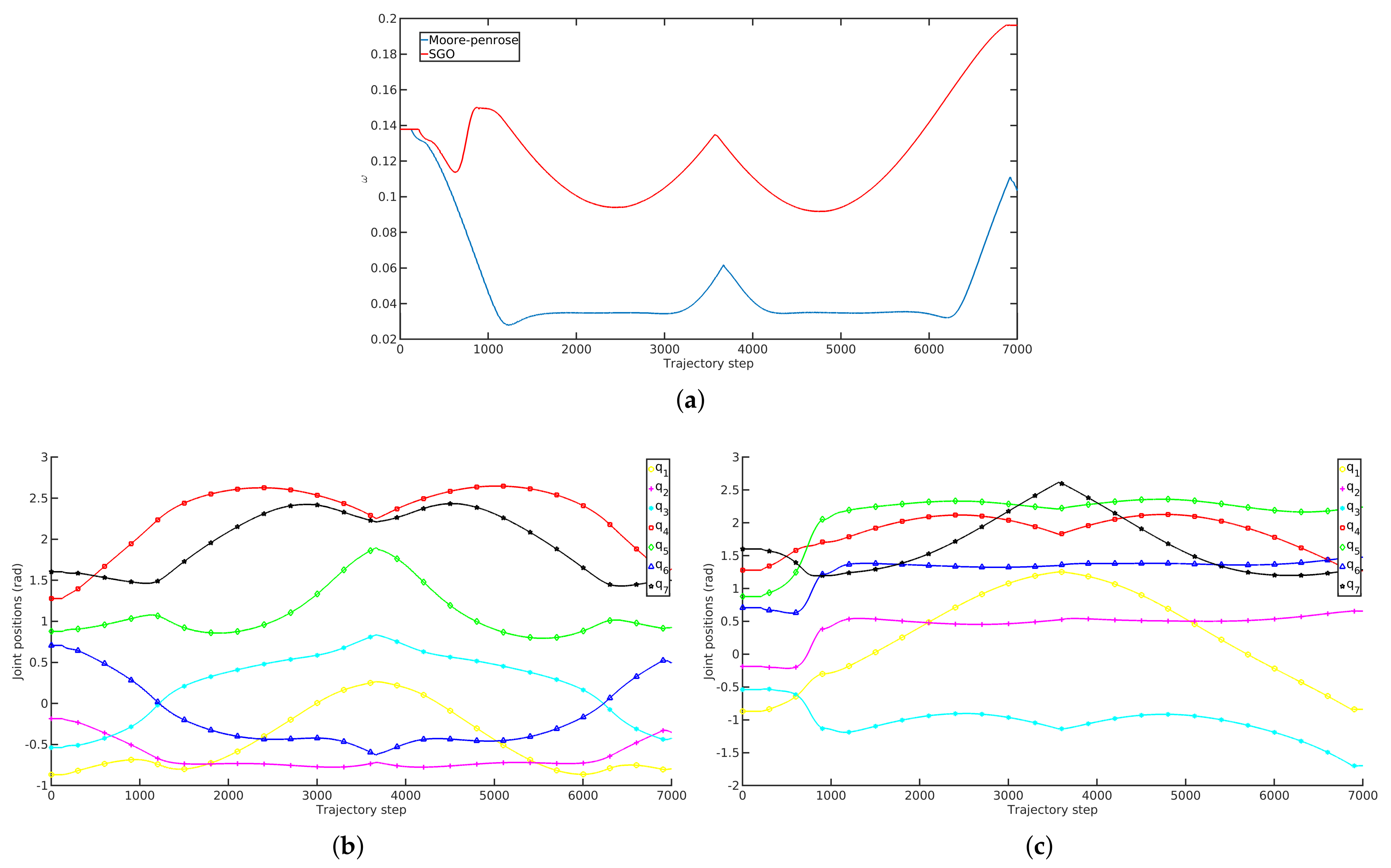
A well-known solution to invert the kinematic Equation (2) is:

$$\dot{\mathbf{q}}=J^{†}\dot{\mathbf{x}},$$

(3)

where $J^{†}$ is the Moore–Penrose pseudo-inverse [20], defined as $J^{†}=J^T{\left(J{J}^T\right)}^{-1}$. This pseudo-inverse has nice properties, since it minimizes the norm $|{\dot{\mathbf{q}}}^T\dot{\mathbf{q}}|$. Thus, given an initial joint position ${\mathbf{q}}_r$, the length of the computed joint trajectory is, by nature, minimal. This equation allows us to compute the joint positions required to reach a set of positions and orientations $G=\{{\mathbf{x}}_1,{\mathbf{x}}_2,\dots ,{\mathbf{x}}_N\}$ of the end effector. This minimum square solution is represented in Algorithm 2. The algorithm, for each time step, generates a joint speed that brings the solution $\mathbf{x}$ closer to the desired goal ${\mathbf{x}}_i$. The final solution of the algorithm depends on the initial seed used ${\mathbf{q}}_r$, thus, infinite solutions can be obtained by initializing ${\mathbf{q}}_r$ randomly. However, this solution may produce a path that includes kinematic singularities [3] or collides with obstacles in the environment. This simple planner makes use of Algorithm 3, computing at each time step the inverse kinematics solution from a given random joint position ${\mathbf{q}}_r$ along the initial trajectory.

Algorithm 2 Simple Planner (G, ${\mathbf{q}}_r$)

INPUT:$G=\{{\mathbf{x}}_1,{\mathbf{x}}_2,\dots {\mathbf{x}}_N\}$, set of positions and orientations

${\mathbf{q}}_r$, an initial random seed for joint positions

OUTPUT:$\{{\mathbf{q}}_1,{\mathbf{q}}_2,\dots ,{\mathbf{q}}_N\}$, the joints configuration path

1: functionSimple_Planner(G) 2:     $\mathbf{q}={\mathbf{q}}_r$ 3:     for $i=1,2,\dots ,N$ do 4:         ${\mathbf{x}}_i$ = $G\left\{i\right\}$ 5:         ${\mathbf{q}}_i$ = Inverse_Kinematics$({\mathbf{x}}_i,\mathbf{q})$ 6:         $\mathbf{q}={\mathbf{q}}_i$ 7:     end for       return $Q=\{{\mathbf{q}}_1,{\mathbf{q}}_2,\dots ,{\mathbf{q}}_N\}$ (the joint path) 8: end function

Algorithm 3 Inverse Kinematics(${\mathbf{x}}_i$, ${\mathbf{q}}_r$)

INPUT:

${\mathbf{x}}_i$, the position and orientation of the end effector

${\mathbf{q}}_r$, the initial seed of the algorithm

OUTPUT:

$\mathbf{q}$, joint positions

1: functionInverse_Kinematics(${\mathbf{x}}_i$, ${\mathbf{q}}_r$) 2:     ${\mathbf{q}}_{\mathbf{i}}={\mathbf{q}}_{\mathbf{r}}$ 3:     while $\mathbf{x}\ne {\mathbf{x}}_i$ do 4:         $\dot{\mathbf{x}}=Compute\_VW({\mathbf{x}}_i,\mathbf{x})$ 5:         $J_i$ = Jacobian(${\mathbf{q}}_i$) 6:         ${\dot{\mathbf{q}}}_i=J_i^{†}\dot{\mathbf{x}}$ 7:         $\mathbf{q}=\mathbf{q}+{\dot{\mathbf{q}}}_i\ast \Delta t$ 8:         $\mathbf{x}=f\left(\mathbf{q}\right)$ 9:     end while 10: return$\mathbf{q}$ 11: end function 12: functionCompute_VW(${\mathbf{x}}_i$, $\mathbf{x}$) 13:     //Computes linear and angular speed 14:     //to reduce the error in $\mathbf{x}-{\mathbf{x}}_i$ 15:     $\dot{\mathbf{x}}=(\mathbf{x}-{\mathbf{x}}_i)/\Delta t$ return $\dot{\mathbf{x}}$ 16: end function

A more general solution to (3) can be written as:

$$\dot{\mathbf{q}}=J^{†}\dot{\mathbf{x}}+(I-J^{†}J){\dot{\mathbf{q}}}_0,$$

(4)

where I is an $(n\times n)$ identity matrix and ${\dot{\mathbf{q}}}_0$ is an arbitrary $(n\times 1)$ joint velocity vector. This solution includes the projector operator $(I-J^{†}J)$, which allows us to project a vector ${\dot{\mathbf{q}}}_0$ on the null space of the initial solution provided by $J^{†}\dot{\mathbf{x}}$. Gradient projection methods exploit this property and compute a joint speed vector $\dot{\mathbf{q}}$ as:

$$\dot{\mathbf{q}}=J^{†}\dot{\mathbf{x}}+(I-J^{†}J)\frac{\partial p_0}{\partial \mathbf{q}}$$

(5)

$p_0$ being an arbitrary cost function that needs to be optimized and $\frac{\partial p_0}{\partial q}$ its gradient. Equation (5) indicates that the redundant degrees of freedom can be used to attain additional constraints, such as obtaining greater manipulability along the trajectory or avoiding collisions with the environment. Usually, manipulability is measured with the index introduced by Yoshikawa [4]:

$$\omega =\sqrt{det\left(J{J}^T\right)}$$

(6)

Additionally, using the manipulability has a strong impact when trying to avoid kinematic singularities. In particular, that situation happens whenever the matrix J, at some joint position $\mathbf{q}$, has a rank less than m. This situation can be easily detected, since the manipulability index $\omega$ becomes null and the manipulator loses, at least, one degree of freedom, which jeopardizes its ability to complete the task.

4. Trajectory Tracking Optimisation

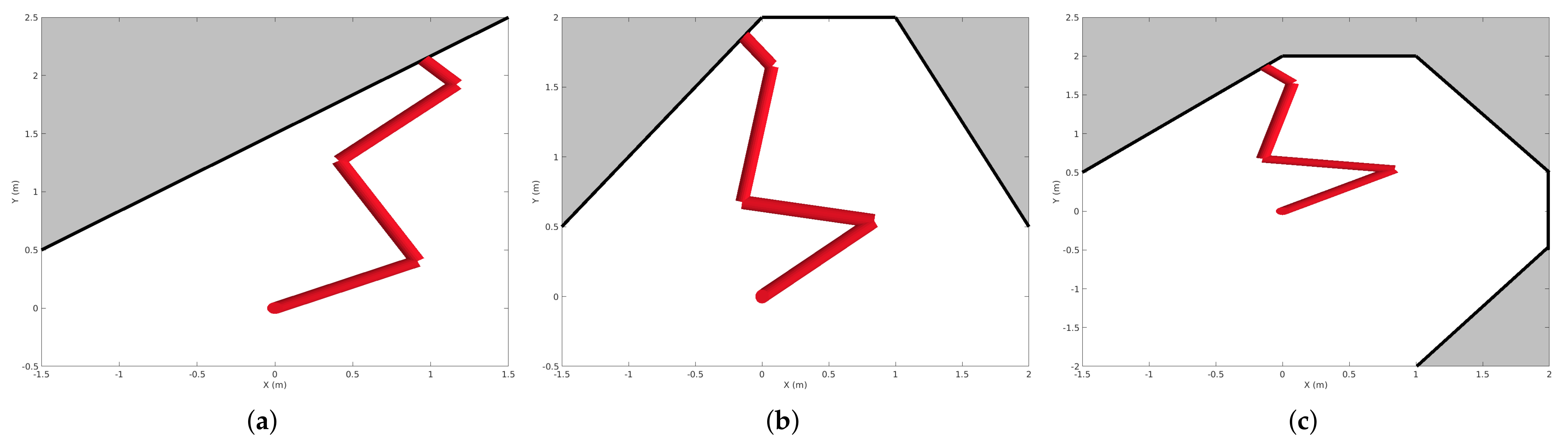
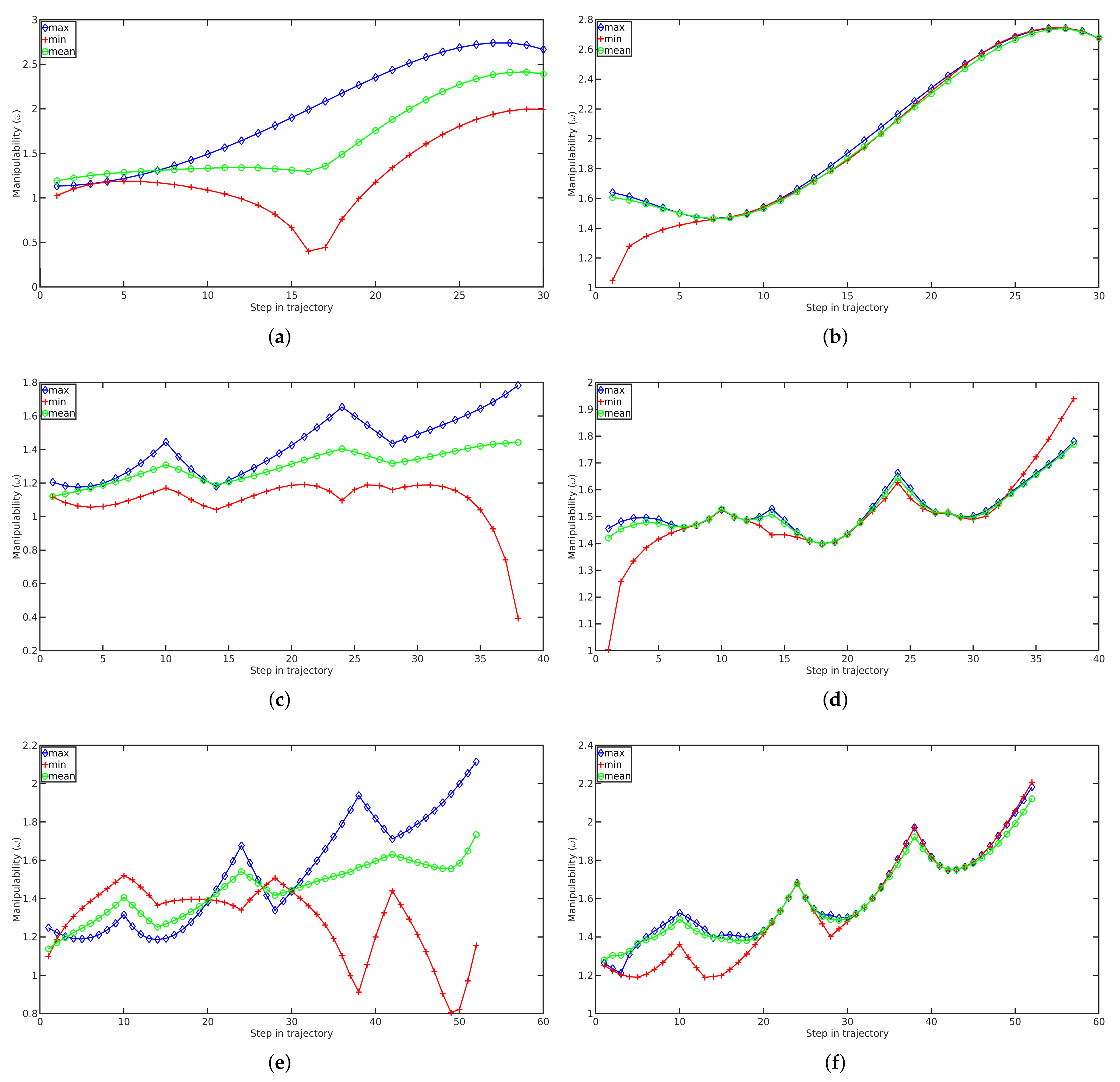
The manipulator task studied in this work corresponds to a tracking problem, whereby an end-effector task space trajectory needs to be mapped to a corresponding joint space trajectory. Given ${\mathbf{x}}_i$, representing the position and orientation of the end effector with respect to a base reference system, the proposed methodology can be regarded as a trajectory optimisation problem for the set of N waypoint goals $G=\{{\mathbf{x}}_1,{\mathbf{x}}_2,\dots {\mathbf{x}}_N\}$ defining the contact surface that the robot must follow with precision. Maximising the manipulability index along the trajectory whilst avoiding obstacles allows us to move away from singularities whilst facilitating the desired motion along the desired surface for the contact/visiting task being pursued.

The method starts by generating a set of K hypotheses on the path:

$$Q_k=\{{\mathbf{q}}_1,{\mathbf{q}}_2\dots {\mathbf{q}}_N\}.$$

(7)

Each hypothesis K of the path ensures that the robot’s end effector reaches the goal ${\mathbf{x}}_i$ for $i=1,\dots N$, and utilises an inverse kinematic method based on the Moore–Penrose pseudo inverse as described in Algorithm 2. The initial joint positions ${\mathbf{q}}_r$ of the manipulator are initialized randomly and, as a result, the resulting K paths $Q_k=\{{\mathbf{q}}_1,{\mathbf{q}}_2\dots {\mathbf{q}}_N\}$ are completely random with the property of $|{\dot{\mathbf{q}}}^T\dot{\mathbf{q}}|$ being minimal for each different trajectory at each time step.

This set of K joint paths form a set of hypotheses that start from different and arbitrary initial ${\mathbf{q}}_1$ joint configurations. Each of the generated trajectories is optimized at each time step $i=1,\dots N$ in order to increase its manipulability index indicated in Equation (6) and, at the same time, avoid obstacles. For each of the K hypotheses over the trajectory, our method performs a sampling on the null space at each step i of the trajectory. The sampling is achieved by generating H samples around each joint configuration ${\mathbf{q}}_i$. To generate each new sample, we compute a vector belonging to the null space as:

$${\dot{\mathbf{q}}}_h=(I-J^{†}J){\dot{\mathbf{q}}}_0,$$

(8)

where ${\dot{\mathbf{q}}}_0$ represents an arbitrary vector that generates a sample of the null space. Next, H random movements are generated as:

$${\mathbf{q}}_h={\mathbf{q}}_i+\alpha ·{\dot{\mathbf{q}}}_h\Delta t.$$

(9)

Any of these new samples ${\mathbf{q}}_h$ around each joint configuration ${\mathbf{q}}_i$ does not alter the position and orientation of the end effector since ${\dot{\mathbf{q}}}_h$ is only a self-motion and thus $J{\dot{\mathbf{q}}}_h=\mathbf{0}$. The variable $\alpha$ is chosen from a normal distribution and $\Delta t$ is an integration time. The time integration step $\Delta t$ and $\alpha$ are parameters of the algorithm.

At each time step, each of the new ${\mathbf{q}}_h$ (for $h=1,\dots H$) is a self motion around the joint positions ${\mathbf{q}}_i$ that can potentially improve its manipulability index while avoiding obstacles. For each ${\mathbf{q}}_h$, we then compute a weight that accounts for the manipulability:

$$\begin{array}{c}\hfill \omega =\sqrt{J{J}^T}\end{array}$$

(10)

$$\begin{array}{c}\hfill c=1/(\omega +\delta )\end{array}$$

(11)

$$\begin{array}{c}\hfill W_{\omega }=e^{\frac{-c}{{\omega }_{max}}},\end{array}$$

(12)

where ${\omega }_{max}$ is the maximum observed manipulability of the mechanism. The parameter $\delta$ avoids the division by zero if the mechanism incurs in a singularity.

In order to consider the presence of obstacles, for each sample ${\mathbf{q}}_h$, we compute the closest distance d of all the points of the robot arm to obstacles and with itself. The distance d is negative whenever any point of the manipulator lies inside an obstacle. We then compute:

$$\begin{array}{c}\hfill x=max(ϵ-d,0)\end{array}$$

(13)

$$\begin{array}{c}\hfill W_o=exp(-x/\lambda ).\end{array}$$

(14)

$ϵ$ is the minimum required distance to the obstacles and $\lambda$ is a parameter that smooths the computed weights. During the experiments we have used $ϵ=0.2$ m and $\lambda =0.5$ m.

A weight is computed that accounts for the manipulability index and the distance to obstacles as:

$$W_{q_h}=W_{\omega }·W_o.$$

(15)

Finally, a sample ${\mathbf{q}}_h$ from the null-space is selected that maximizes the weight $W_{q_h}$. The final path of the robot is obtained by selecting the path with the higher weight $W_{q_h}$. The complete algorithm is described in Algorithm 4.

Algorithm 4 Stochastic Planner(G, O)

INPUT:

$G={\mathbf{x}}_1,{\mathbf{x}}_2,\dots {\mathbf{x}}_N$, set of positions and orientations.

OUTPUT:

$Q={\mathbf{q}}_1,{\mathbf{q}}_2,\dots {\mathbf{q}}_N$, path of the robot.

1: functionStochasticPlanner(G, O) 2:     //Build K initial random paths. 3:     for $k=1,2,\dots ,K$ do 4:         ${\mathbf{q}}_r=uniform(1,m)$ 5:         for $i=1,2,\dots ,N$ do 6:            ${\mathbf{q}}_{i+1}$ = InverseKinematics(${\mathbf{x}}_i$, ${\mathbf{q}}_i$) 7:         end for 8:         //Store a random path for the K particle. 9:         $Q_k=\{{\mathbf{q}}_1,{\mathbf{q}}_2,\dots ,{\mathbf{q}}_N\}$ 10:     end for 11:     while convergence of $\sum W_k$ do 12:         for $k=1,2,\dots ,K$ do 13:            $p_k$ = $G_k$ 14:            for $i=1,2,\dots ,N$ do 15:                $q_i$ = SampleFromNullSpace($G_{k,i}$) 16:                $w_h$ = ComputeWeights($q_h$) 17:                //Find $\mathbf{q}$ that maximizes $W=\{w_1,\dots w_H\}$ 18:                $\widehat{\mathbf{q}}$ = $argma{x}_{q_h}\left(W_h\right)$ 19:                //Add $\widehat{\mathbf{q}}$ to the path 20:            end for 21:         end for 22:     end while 23: return$Q=\{{\mathbf{q}}_1,{\mathbf{q}}_2,\dots ,{\mathbf{q}}_N\}$, the joint path 24: end function 25: functionSampleFromNullSpace($G_{k,i}$) INPUT: Current joint position i at path k. OUTPUT: H samples $q_h$ from null space. 26:     for $h=1,2,\dots ,H$ do 27:           ${\dot{\mathbf{q}}}_h=(I-J^{†}J){\dot{\mathbf{q}}}_0$ 28:           ${\mathbf{q}}_h={\mathbf{q}}_i+ϵ·{\dot{\mathbf{q}}}_h\Delta t$ 29:     end for       return $q_h=\{q_1,q_2,\dots ,q_H\}$, samples from null space. 30: end function

5. Results

The proposed approach is hereby demonstrated through both simulation with a 4DoF planar manipulator, and experimentally on a real robot—the 7R Rethink Robotics Sawyer manipulator. The simulations have been performed in Matlab using the ARTE toolbox (freely available at https://arvc.umh.es/arte, last accessed on 11 November 2021).

5.1. Preliminaries

During all the experiments, the robot’s end effector must be able to achieve a given position and orientation inside the workspace thus ensuring a precise contact with the surface that allows us to complete a hypothetical surface treatment task (polishing, deburring etc.). The details of the two different robots are given next.

• A simulated 4DoF planar robot (shown in Figure 1 in the three simulated workspaces first considered): This robot is composed of four rotational joints and four links of lengths $l_1=l_2=l_3=1$ m and $l_4=0.3$ m. The robot is used to track a line defined in the workspace. The robot end effector must thus reach a set of goal points in the workspace ${\mathbf{x}}_i=(x_i,y_i,{\varphi }_i)$ with $i=1,\dots ,N$ representing the different task goals $(x_i,y_i)$, and a given orientation ${\varphi }_i$ set to remain always perpendicular to the 1D surfaces (lines) to be traced. Since the robot has 4DoF, there exists a free degree of freedom. At each step i, our proposed algorithm will compute the robot’s path q exploiting the null space of the previous task point as described in Section 4.
• A real 7DoF manipulator: The Sawyer robot, by Rethink Robotics, is composed of seven rotational joints. The manipulator is made to follow a virtual straight path that lies exactly on a surface. Thus, the robot end effector must be capable of visiting a set of positions defined by ${\mathbf{x}}_i$ with $i=1,\dots N$ that sit on the surface, and do so with an orientation of the end effector perpendicular to the surface. Since the robot has 7DoF, there exists a free degree of freedom. Again, at each time step i, our proposed algorithm will compute the robot’s path ${\mathbf{q}}_i$, exploiting the null space of the previous task point just visited.

During the experiments, our proposed algorithm will be used to find a trajectory that is able to complete the required task while, at the same time, optimising the manipulability at each time step and avoiding collisions.

5.2. Simulation Study

Three different case studies have been carried out in simulation with the same 4DoF planar manipulator. The workspace has been made to be increasingly challenging to test the effectiveness of the scheme under controlled but demanding conditions:

• Case study I: In order to complete the task, the robot must follow a trajectory perpendicular to the given surface shown in Figure 1a. During the trajectory the robot must not collide with the surface or with itself. This restriction imposes that any point belonging to links 1, 2 and 3 must be at a distance higher than $\delta =0.2$ m to the surface. In addition, any joint in the robot must be at a distance higher than $\delta =0.2$ m from any other joint center;
• Case study II: In this simulation, the same restrictions considered in case study I apply. However, the surface path to be tracked is made more demanding, as can be seen in Figure 1b. The changes in the normal to the surfaces are accomplished by a set of smooth changes;
• Case study III: As above, but a workspace with a near-full overhang around the robot makes tracking particularly challenging for collision checking during the surface following task, almost encroaching the robot fully by its surroundings and severely limiting its mobility, as depicted in Figure 1c.

An extensive set of runs has been carried out in order to compare the outcome of our proposed approach. For each trajectory produced by the algorithm, the mean manipulability value is computed as $\widehat{\omega }=(1/N)\sum w_i$, considering that the trajectory has N different waypoints. In addition, the whole trajectory is computed to check for collisions with the environment and self-collisions. The success rate accounts for the number of generated trajectories that do not collide with any obstacle.

Figure 2 presents the results in terms of manipulability at each time step along the single line environment (case studies I, II and III). For all graphs, the blue line represents the joint trajectory that possesses the higher mean manipulability that the algorithm can achieve. The trajectory with minimum mean manipulability is also shown in red, whilst green presents a trajectory that lies in the mean value of all the manipulabilities obtained. We compare the results of the proposed Stochastic Constrained Optimization (SCO) method on the right (Figure 2b,d,f) with the output of Algorithm 2 on the left (Figure 2a,c,e), representing the path solution recovered from an inverse kinematic solution based on the Moore–Penrose pseudo inverse. The initial position ${\mathbf{q}}_r$ used for this algorithm is selected randomly. It is clearly apparent how SCO is able to consistently produce trajectories that attain a higher degree of manipulability along the trajectory, while, at the same time, accomplishing the task at hand. Please, note also the low dispersion achieved in the manipulabilities represented in Figure 2b,d,f, indicative of the dependable ability of SCO to produce high manipulability regardless.

Table 1. Results of case studies I, II and III.

Case	K	N	Success Rate (%)	Manip. Mean $\widehat{\mathit{\omega }}$	Manip. Max.	Comp. Time (Sec.)
I A
( Simple_Planner)	-	2000	44	1.64 ± 0.48	1.95	0.99 ± 0.01
I B	1	30	76	1.96 ± 0.16	2.04	4.32 ± 0.11
I B	5	30	90	1.98 ± 0.11	2.04	13.38 ± 0.17
I B	10	30	96	2.01 ± 0.05	2.04	24.27 ± 0.62
I B	20	30	100	2.02 ± 0.03	2.04	45.92 ± 2.13
I B	50	30	100	2.03 ± 0.02	2.28	114.18 ± 2.25
II A
( Simple_Planner)	-	2000	26	1.29 ± 0.21	1.41	0.56 ± 0.01
II B	1	30	56	1.47 ± 0.12	1.52	4.99 ± 0.12
II B	5	30	80	1.49 ± 0.13	1.52	17.18 ± 0.19
II B	10	30	100	1.50 ± 0.06	1.52	34.66 ± 0.74
II B	20	30	100	1.52 ± 0.02	1.53	64.74 ± 3.33
II B	50	30	100	1.53 ± 0.006	1.53	156.64 ± 4.62
III A
( Simple_Planner)	-	2000	12	1.20 ± 0.43	1.61	0.77 ± 0.01
III B	1	30	33	1.58 ± 0.05	1.60	6.37 ± 0.18
III B	5	30	80	1.58 ± 0.06	1.61	23.63 ± 0.66
III B	10	30	97	1.60 ± 0.05	1.61	44.85 ± 0.77
III B	20	30	100	1.60 ± 0.03	1.61	88.99 ± 3.15
III B	50	30	100	1.61 ± 0.009	1.61	219.88 ± 4.68

presents the results of case studies I, II and III. The first row of each simulation, named “Simple Planner”, represents the results obtained using Algorithm 2 when applied to each of the workspaces represented in Figure 1. The following rows, represent the results of the SCO algorithm with varying number of samples K. In order to evaluate the success rate, we check that the robot does not collide with obstacles or derives in self-collision during the resulting trajectory. As expected, the success rate of this algorithm is low during the three simulations. In addition, it also produces trajectories that exhibit low manipulability overall along the path. The first row of simulation IB uses the proposed SCO Algorithm 4 using a single hypothesis on the path ($K=1$). In this case, the planner is able to produce a significantly higher success rate (76%) compared to Algorithm 2 (simple planner). In addition, the trajectory is optimized, both avoiding obstacles and increasing the mean manipulability. As the number of hypotheses K increases, we observe a higher success rate, while, at the same time, increasing the manipulability along the whole trajectory. It is worth noting that, for $K=10$ hypotheses, the proposed algorithm achieves a success rate of 100%. Further increasing $K=20,50$ hypotheses maintains the same success rate and allows us to obtain an even higher manipulability index along the trajectories.

Table 1 also presents the results of case study II. As before, the “Simple Planner” in the first row refers to the results of the path obtained with Algorithm 2, where the simulation samples the path at a total of $N=2000$ and, for a successful run, collisions with itself and the environment for a given trajectory must be avoided. The success rate of this algorithm is, again, very low. Given the increased complexity of the task when compared to run IA, the success rate is even lower. The results with SCO are collected under case study IIB, and as below different cases are investigated with varying initial hypotheses along the path: $K=\{1,5,10,20,30\}$. It can be observed how the proposed SCO is successful in producing a 56% of feasible solutions for $K=1$ and 80% for $K=5$, a marked improvement over the “Simple Planner” even with these low number of hypotheses. Moreover, as the number of hypotheses K increases, so does the success rate, while, at the same time, increasing the manipulability along the length of the trajectory. It is worth noting that, for $K=10$, the proposed algorithm is able to achieve full success (rate of 100%). Further increasing K to 20 or 50 maintains flawless success and allows us to obtain even marginally higher manipulability along the trajectories. Table 1 also collects the results of case study III. As before, “Simple Planner” in the first row refers to the results of the path obtained with Algorithm 2. The success rate of this algorithm is, again, very low. The task in case study III is more demanding, which explains the low success rate, compared to case studies IA and IIA. Again, the results with SCO are collected under simulation IIIB with $K=\{1,5,10,20,30\}$. Following the same trends observed before, the proposed SCO produces a 33% of successful solutions for $K=1$ and 80% for $K=5$. The proposed algorithm also succeeds in this more demanding scenario, and as the number of hypotheses K increases, the success rate and the manipulability are increased. It is worth noting that for $K=20$ the proposed algorithm is able to achieve full success (rate of 100%). As observed earlier, further increasing K beyond this point (to the maximum of 50 hypotheses in this case) only slightly increases the optimized manipulability while maintaining the same success rate.

Table 1 also presents computation times of each simulation carried out on an Intel^™ Core i7 CPU @ 2.90GHz × 16 running Ubuntu 20.04 and Matlab^™ R2018a. Mean computation times (seconds) and $2\sigma$ intervals are collected. As expected, a linear trend is observed in the computational effort.

5.3. Real Experiments

An experiment has been conducted on a physical manipulator to verify the performance of the proposed method under realistic settings. Figure 3 presents the real experimental setup with the 7R Rethink Robotics Sawyer cobot. The experiment consists of tracking a reference linear path on a flat surface whist keeping the tool in an orientation perpendicular to the surface throughout the motion. A force controller developed to maintain contact with the surface was implemented [18] to aid with the task at hand of simulating a surface conditioning assignment such as polishing, whilst the pose adopted along the path is set by the proposed SCO path planning strategy. The experimental setup is depicted in Figure 3a, consisting of a 7R Rethink Robotics Sawyer cobot, a force sensor Nano25 SI-25-25 attached to the robot end-effector, a small polishing tool proxy attached to the sensor (a cylinder of 43 × 43 × 10 mm), and a target flat surface to polish.

As per the test methodology adopted in the simulation cases to show the capabilities of the proposed method, the routine undertaken includes a comparison with the standard “Simple Planner” derived from the the Moore–Penrose solution (Algorithm 2). The initial conditions are set to be the same in both cases: an obstacle-free initial pose with average manipulability established prior. This was the initial condition fed to both trajectory planners. A video is supplied (https://arvc.umh.es/arte/AppliedSciences21.mp4, accessed on 11 November 2021) to visualise the full experimental setting and resulting motion, with several stills depicting the starting, mid- and end-points of the test trajectories also being collected in Figure 3. It can be observed how the optimality in manipulability being sought out by the SCO proposed planners derives configurations that keep the elbow link down, whereas in the “Simple Planner” case that is not the case, ultimately even compromising stability by traversing near-singular regions. The reader is referred to the video linked in the manuscript where the undesirable dynamic disturbances induced in the controller are clearly apparent with vibrations at compromised locations along the path, most notably at the mid-point (Figure 3e).

The final manipulability attained in both instances, shown in Figure 4, corroborates the ability of the algorithm to seek areas with higher manipulability, hence permitting operations with manipulator configurations away from singularity regions, ultimately leading to superior end-effector precision, less energy expenditure and overall safer trajectories whilst seeking to abide by the desired end effector path during execution.

6. Conclusions

An efficient stochastic algorithm able to produce obstacle-free configuration trajectories for a given workspace has been proposed. The random process exploits the particular kinematics of closed-chain mechanisms with redundant actuation to increase manipulability along a desired end-effector task-space motion in an iterative process. The stochastic solution remains close to optimal whilst affording computational tractability, being an attractive proposition for implementation on real robots. Results from tests in challenging simulation scenarios, as well as with a 7R manipulator constrained to undertake surface treatment tasks, have been presented to show the suitability of the proposed Stochastic Constrained Optimization (SCO) trajectory planner for redundant manipulators to be able to track arbitrary task-space paths. The challenging aspect of planning trajectories, where the robot must remain in close contact with non-smooth irregular surfaces whilst optimizing the manipulability index at each time step, represents an on-going research effort continuing with the line of work presented in this manuscript.

References

1. Sciavicco, L.; Siciliano, B. Modelling and Control of Robot Manipulators, 2nd ed.; Springer: London, UK, 2000. [Google Scholar]
2. Zlatanov, D.; Fenton, R.G.; Benhabib, B. Singularity analysis of mechanisms and robots via a motion-space model of the instantaneous kinematics. In Proceedings of the 1994 IEEE International Conference on Robotics and Automation, San Diego, CA, USA, 8–13 May 1994; pp. 980–985. [Google Scholar] [CrossRef]
3. Siciliano, B.; Slotine, J. A general framework for managing multiple tasks in highly redundant robotic systems. In Proceedings of the Fifth International Conference on Advanced Robotics (ICAR’91), Pisa, Italy, 19–22 June 1991; pp. 1211–1216. [Google Scholar]
4. Yoshikawa, T. Manipulability of Robotic Mechanisms. Int. J. Robot. Res. 1985, 4, 3–9. [Google Scholar] [CrossRef]
5. Solanes, J.E.; Gracia, L.; Muñoz-Benavent, P.; Valls Miro, J.; Girbés, V.; Tornero, J. Human-robot cooperation for robust surface treatment using non-conventional sliding mode control. ISA Trans. 2018, 80, 528–541. [Google Scholar] [CrossRef] [PubMed]
6. Quispe, A.H.; Stilman, M. Deterministic Motion Planning for redundant robots along End-Effector Paths. In Proceedings of the 2012 IEEE-RAS International Conference on Humanoid Robots, Osaka, Japan, 29 November–1 December 2012; pp. 785–790. [Google Scholar] [CrossRef]
7. Nakamura, Y.; Hanafusa, H. Optimal Redundancy Control of Robot Manipulators. Int. J. Robot. Res. 1987, 6, 32–42. [Google Scholar] [CrossRef]
8. Scoccia, C.; Palmieri, G.; Palpacelli, M.C.; Callegari, M. A Collision Avoidance Strategy for Redundant Manipulators in Dynamically Variable Environments: On-Line Perturbations of Off-Line Generated Trajectories. Machines 2021, 9, 30. [Google Scholar] [CrossRef]
9. Palmieri, G.; Scoccia, C. Motion Planning and Control of Redundant Manipulators for Dynamical Obstacle Avoidance. Machines 2021, 9, 121. [Google Scholar] [CrossRef]
10. Bottin, M.; Rosati, G. Trajectory Optimization of a Redundant Serial Robot Using Cartesian via Points and Kinematic Decoupling. Robotics 2019, 8, 101. [Google Scholar] [CrossRef] [Green Version]
11. Ratliff, N.; Zucker, M.; Bagnell, J.A.; Srinivasa, S. CHOMP: Gradient optimization techniques for efficient motion planning. In Proceedings of the 2009 IEEE International Conference on Robotics and Automation, Kobe, Japan, 12–17 May 2009; pp. 489–494. [Google Scholar] [CrossRef] [Green Version]
12. Kalakrishnan, M.; Chitta, S.; Theodorou, E.; Pastor, P.; Schaal, S. STOMP: Stochastic trajectory optimization for motion planning. In Proceedings of the 2011 IEEE International Conference on Robotics and Automation, Shanghai, China, 9–13 May 2011; pp. 4569–4574. [Google Scholar] [CrossRef]
13. LaValle, S.M.; Kuffner, J.J. Randomized kinodynamic planning. In Proceedings of the IEEE International Conference on Robotics and Automation, Detroit, MI, USA, 10–15 May 1999; pp. 473–479. [Google Scholar]
14. Kuffner, J.; LaValle, S. RRT-connect: An efficient approach to single-query path planning. In Proceedings of the 2000 ICRA—Millennium Conference—IEEE International Conference on Robotics and Automation, Symposia Proceedings (Cat. No.00CH37065), San Francisco, CA, USA, 24–28 April 2000; Volume 2, pp. 995–1001. [Google Scholar] [CrossRef] [Green Version]
15. Berenson, D.; Srinivasa, S.; Kuffner, J. Task Space Regions: A framework for pose-constrained manipulation planning. Int. J. Robot. Res. 2011, 30, 1435–1460. [Google Scholar] [CrossRef]
16. Cefalo, M.; Oriolo, G.; Vendittelli, M. Planning safe cyclic motions under repetitive task constraints. In Proceedings of the 2013 IEEE International Conference on Robotics and Automation, Karlsruhe, Germany, 6–10 May 2013; pp. 3807–3812. [Google Scholar] [CrossRef]
17. Oriolo, G.; Cefalo, M.; Vendittelli, M. Repeatable Motion Planning for Redundant Robots Over Cyclic Tasks. IEEE Trans. Robot. 2017, 33, 1170–1183. [Google Scholar] [CrossRef]
18. Solanes, J.E.; Gracia, L.; Muñoz-Benavent, P.; Esparza, A.; Valls Miro, J.; Tornero, J. Adaptive robust control and admittance control for contact-driven robotic surface conditioning. Robot.-Comput.-Integr. Manuf. 2018, 54, 115–132. [Google Scholar] [CrossRef]
19. Mayorga, R.V.; Wong, A.K.C. On the Optimal Path Planning for Robot Manipulators. In Kinematic and Dynamic Issues in Sensor Based Control; Taylor, G.E., Ed.; Springer Berlin Heidelberg: Berlin/Heidelberg, Germany, 1990; pp. 179–200. [Google Scholar]
20. Moore, E.H. On the Reciprocal of the General Algebraic Matrix. Bull. Am. Math. Soc. 1920, 26, 394–395. [Google Scholar] [CrossRef]
Figure 1. Workspaces for simulation experiments. Experiment I (a), Experiment II (b) and Experiment III (c). The manipulator fixed base is located at the ( 0 , 0 ) coordinates. The dark grey sections define the obstacle walls, with its surface identifying the contact line to be tracked by the manipulator end effector.
Applsci 11 10636 g001
Figure 2. A comparison of the manipulability metric evolution for case studies I, II and III. Cases IA, IIA and IIIA were carried out over a total of N = 2000 sample waypoints along the desired task-space trajectory. The blue line represents the trajectory that presents the maximum value in terms of mean manipulability along the line that the algorithm is able to achieve, red is the minimum and green the mean value across all the runs. The corresponding simulations IB, IIB and IIIB were obtained by using SCO with K=20 samples. (a) Case study I A, (b) Case study I B, (c) Case study II A, (d) Case study II B, (e) Case study III A, (f) Case study III B.
Applsci 11 10636 g002
Figure 3. Sawyer polishing task experiment: (a) setup: 7R manipulator with a force sensor attached to the robot end-effector, a tool consisting of a cylinder of 43 × 43 × 10 mm attached to the sensor and a flat surface target, (b) initial pose with minimal manipulability for both tests, (c,d) proposed SCO algorithm, (e,f) “Simple Planner” case.
Applsci 11 10636 g003
Figure 4. Real polishing experiment with the Sawyer robot: (a) Manipulability comparison: attained manipulability evolution of the traversed path illustrated in Figure 3, with the proposed SCO scheme shown in red (top line), and the “Simple Case” Moore–Penrose solution depicted in blue (bottom line). Corresponding (b) “Simple Planner” trajectory evolution, and (c) Evolution of joint trajectories using the SCO algorithm.
Applsci 11 10636 g004