
Buckling Analysis of Piles in Multi-Layered Soils


Abstract
:1. Introduction
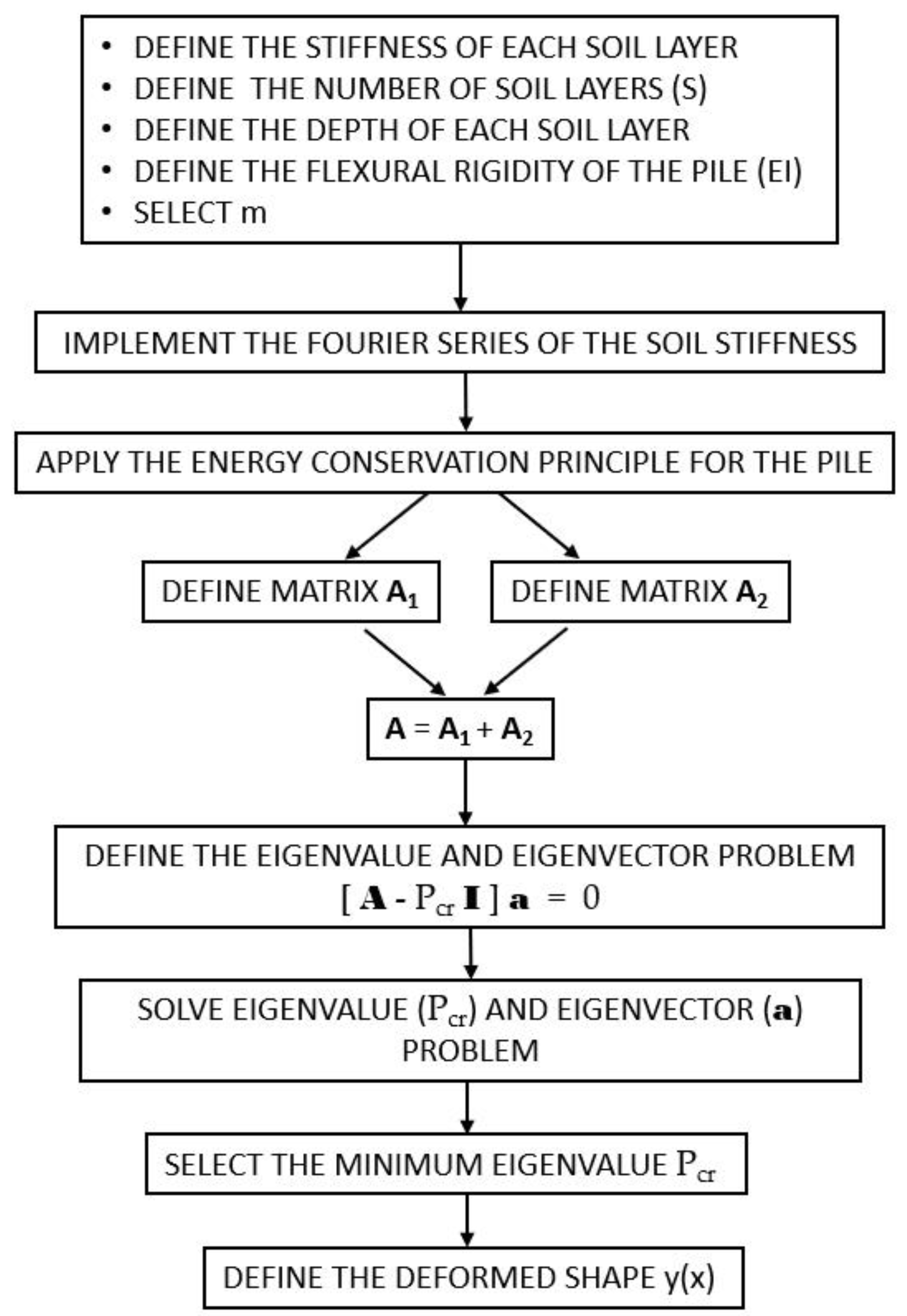
2. Methodology
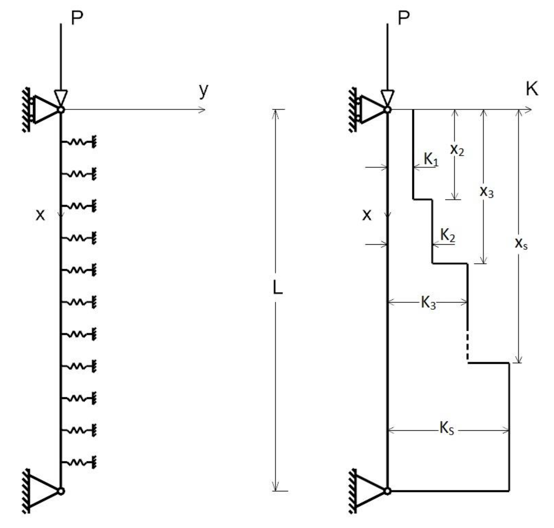
2.1. Formulation of the Problem
2.2. Conditions for Minimum P
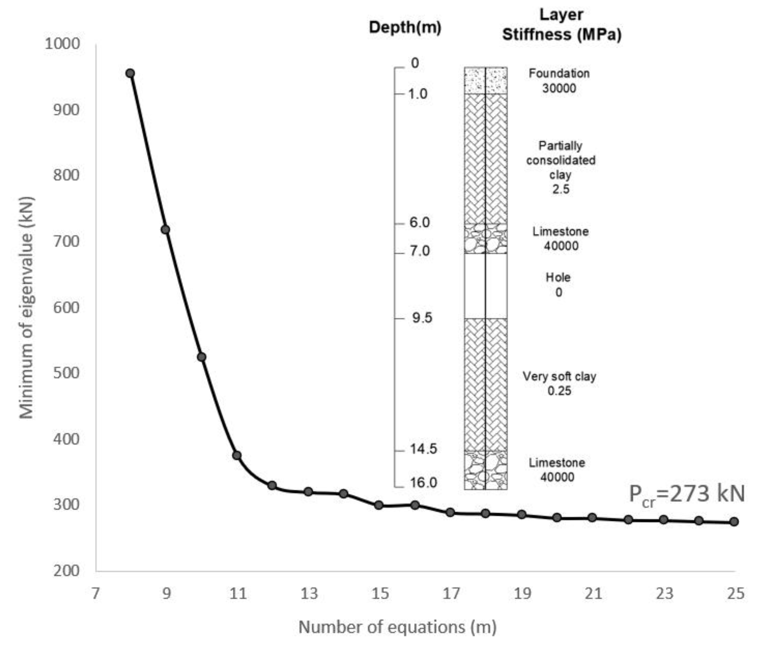
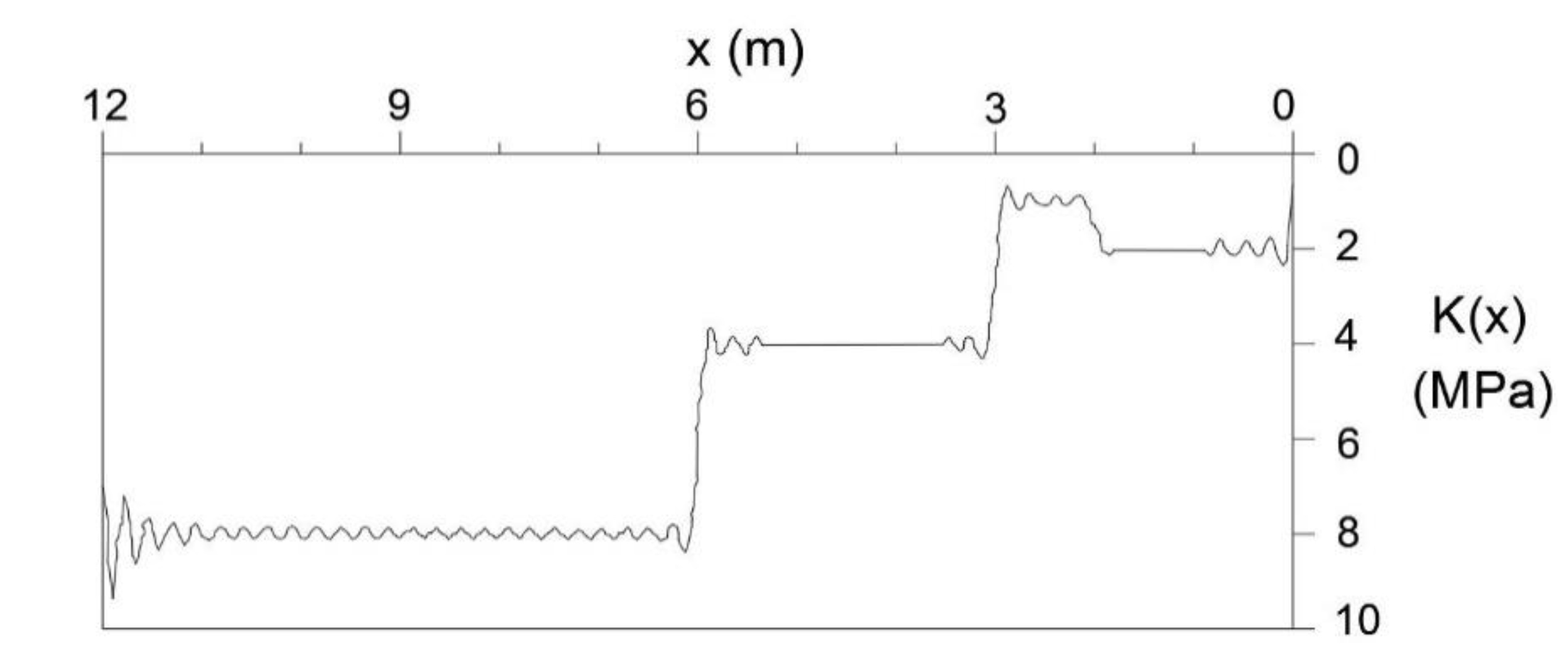
3. Discussion and Results
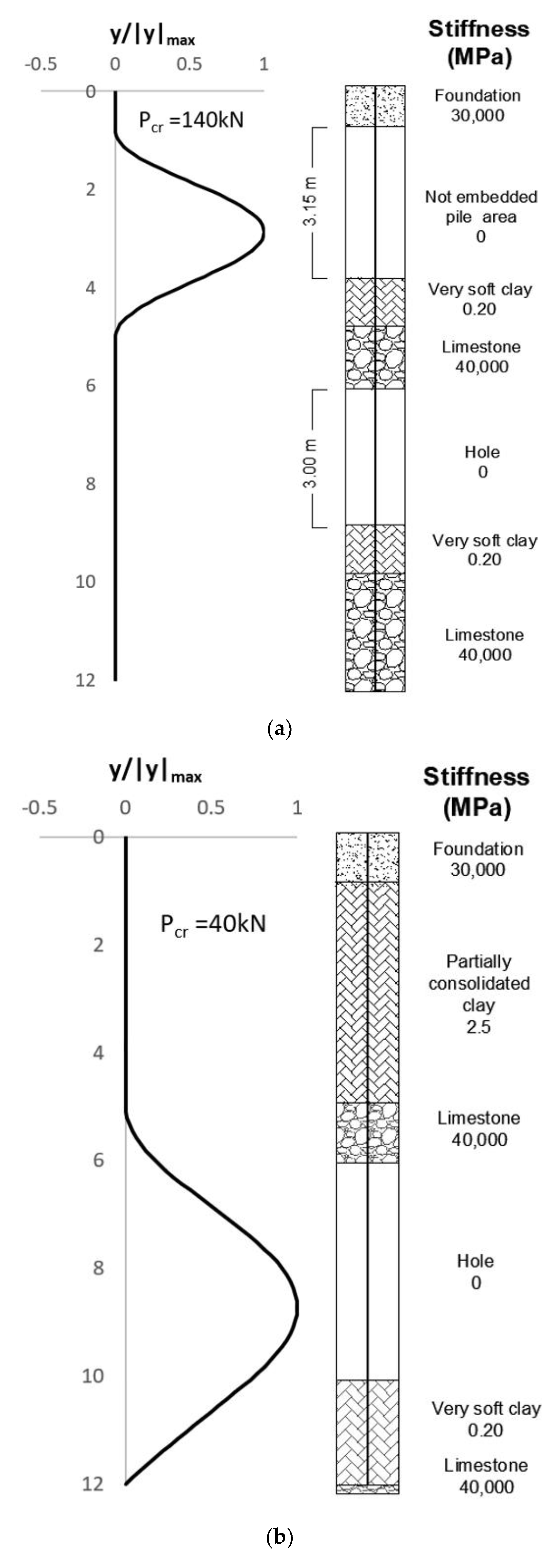
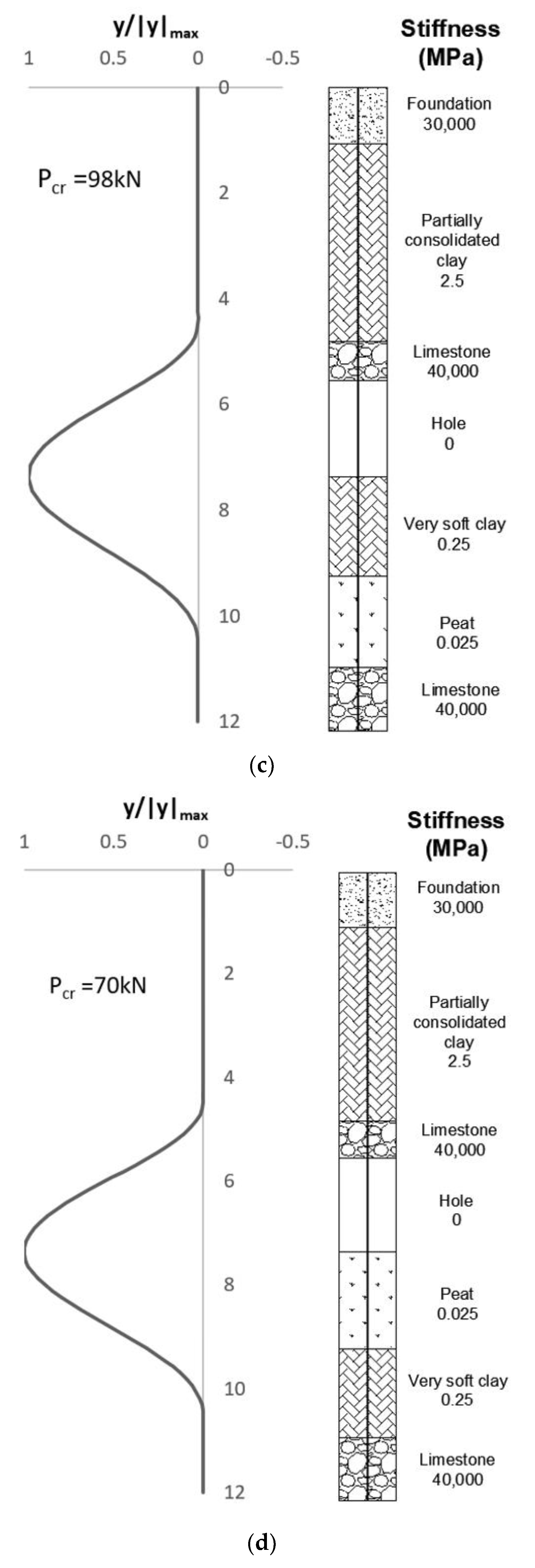
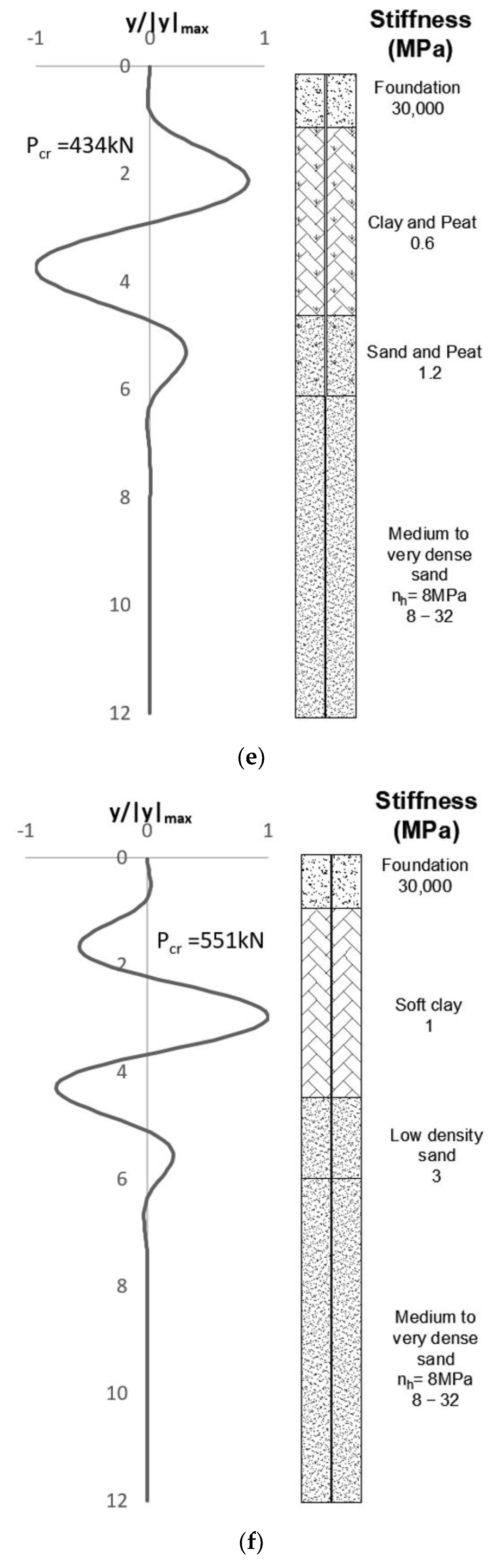
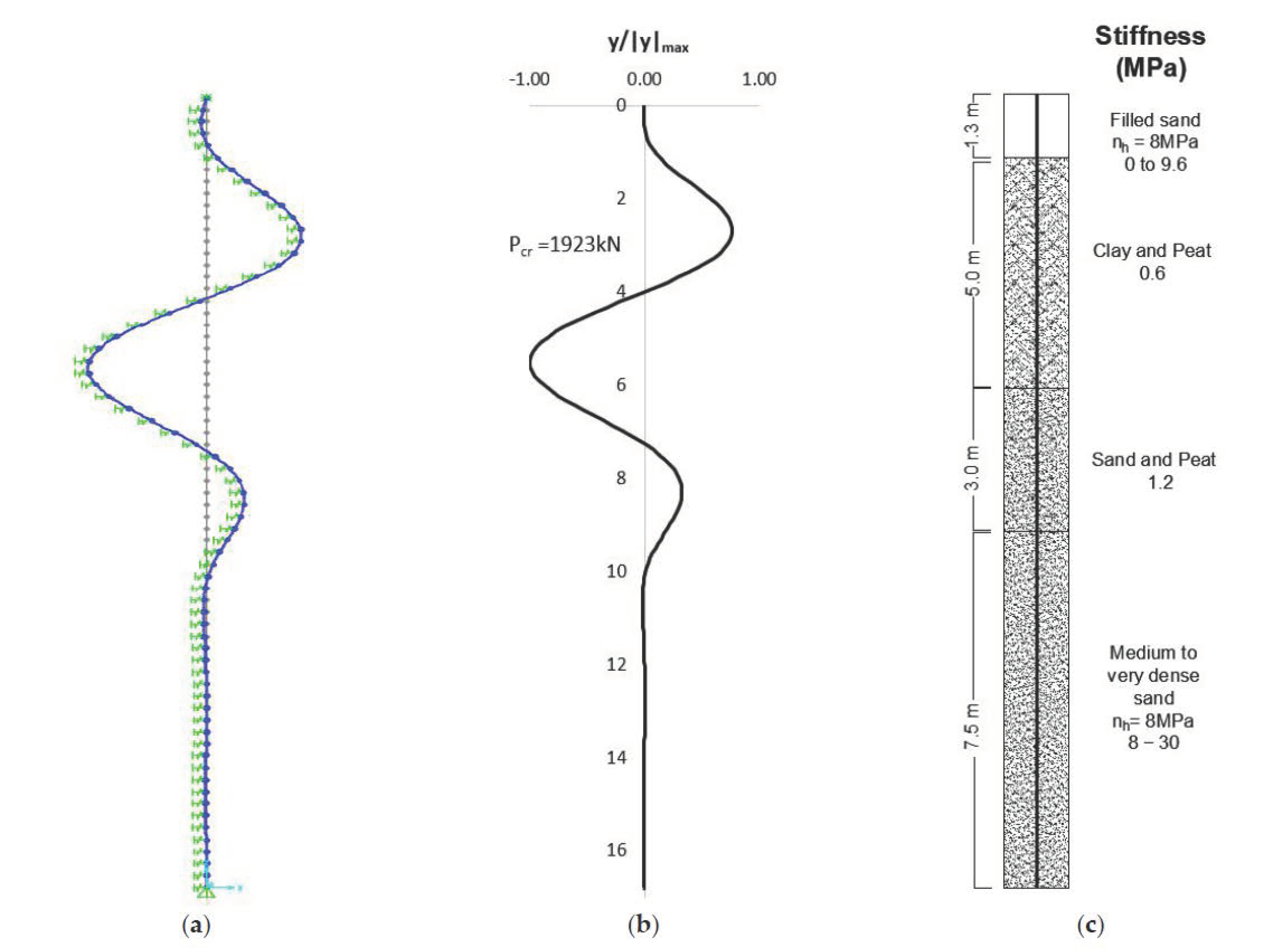
3.1. Applications and Validations
4. Conclusions
Author Contributions
Funding
Conflicts of Interest
References
- Madhav, M.R.; Davis, E.H. Buckling of Finite Beams in Elastic Continuum. ASCE J. Eng. Mech. Div. 1974, 100, 1227–1236. [Google Scholar] [CrossRef]
- Poulos, H.G.; Davis, E.H. Pile Foundation Analysis and Design; John Wiley & Sons, Inc.: New York, NY, USA, 1980. [Google Scholar]
- Timoshenko, S.P.; Gere, J.M.; Prager, W. Theory of Elastic Stability, Second Edition. J. Appl. Mech. 1962, 29, 220–221. [Google Scholar] [CrossRef]
- Gabr, M.; Wang, J.J.; Zhao, M. Buckling of Piles with General Power Distribution of Lateral Subgrade Reaction. J. Geotech. Geoenviron. Eng. 1997, 123, 123–130. [Google Scholar] [CrossRef]
- Shields, D.R. Buckling of Micropiles. J. Geotech. Geoenviron. Eng. 2007, 133, 334–337. [Google Scholar] [CrossRef]
- Bergfelt, A. The axial and lateral load bearing capacity, and failure by buckling of piles in soft clay. In Proceedings of the 4th International Conference on Soil Mechanics and Foundation Engineering, London, UK, 12–24 August 1957; Butterworths Scientific Publications: London, UK, 1957; pp. 8–13. [Google Scholar]
- U.S. Department of Transportation. Federal Highway Administration Micropile Design and Construction Guidelines FHWA-SA-97-070; U.S. Department of Transportation: Washington, DC, USA, 2005. [Google Scholar]
- Hegazy, A.A.E. Analysis of buckling load micropiles embedded in a weak soil under vertical axial loads. Int. J. Civ. Eng. (IJCE) 2014, 3, 155–166. [Google Scholar]
- Ofner, R.; Wimmer, H. Buckling resistance of micropiles in varying soil layers. Bautechnik 2007, 84, 881–890. [Google Scholar] [CrossRef]
- British Standards Institution. EN 1993 Eurocode 3: Design of Steel Structures; British Standards Institution: London, UK, 2005; Volume 1. [Google Scholar]
- British Standards Institution. EN 1997 Eurocode 7: Geotechnical Design—Part 1: General Rules; British Standards Institution: London, UK, 2011; Volume 1. [Google Scholar]
- Vogt, N.; Vogt, S.; Kellner, C. Buckling of slender piles in soft soils. Bautechnik 2009, 86, 98–112. [Google Scholar] [CrossRef]
- Bhattacharya, S.; Goda, K. Probabilistic buckling analysis of axially loaded piles in liquefiable soils. Soil Dyn. Earthq. Eng. 2013, 45, 13–24. [Google Scholar] [CrossRef]
- Dash, S.R.; Bhattacharya, S.; Blakeborough, A. Bending-buckling interaction as a failure mechanism of piles in liquefiable soils. Soil Dyn. Earthq. Eng. 2010, 30, 32–39. [Google Scholar] [CrossRef]
- Zhang, X.; Tang, L.; Li, X.; Ling, X.; Chan, A. Effect of the combined action of lateral load and axial load on the pile instability in liquefiable soils. Eng. Struct. 2020, 205, 110074. [Google Scholar] [CrossRef]
- Tang, L.; Man, X.; Zhang, X.; Bhattacharya, S.; Cong, S.; Ling, X. Estimation of the critical buckling load of pile foundations during soil liquefaction. Soil Dyn. Earthq. Eng. 2021, 146, 106761. [Google Scholar] [CrossRef]
- Bhattacharya, S.; Adhikari, S.; Alexander, N.A. A simplified method for unified buckling and free vibration analysis of pile-supported structures in seismically liquefiable soils. Soil Dyn. Earthq. Eng. 2009, 29, 1220–1235. [Google Scholar] [CrossRef]
- Vega-Posada, C.A.; Gallant, A.P.; Areiza-Hurtado, M. Simple approach for analysis of beam-column elements on homogeneous and non-homogeneous elastic soil. Eng. Struct. 2020, 221, 111110. [Google Scholar] [CrossRef]
- Khedmatgozar Dolati, S.S.; Mehrabi, A. Review of available systems and materials for splicing prestressed-precast concrete piles. Structures 2021, 30, 850–865. [Google Scholar] [CrossRef]
- Farhangi, V.; Karakouzian, M.; Geertsema, M. Effect of micropiles on clean sand liquefaction risk based on CPT and SPT. Appl. Sci. 2020, 10, 3111. [Google Scholar] [CrossRef]
- Farhangi, V.; Karakouzian, M. Design of Bridge Foundations Using Reinforced Micropiles. In Proceedings of the International Road Federation Global R2T Conference & Expo, Las Vegas, NV, USA, 19–22 November 2019. [Google Scholar]
- Lan, C.; Briseghella, B.; Fenu, L.; Xue, J.; Zordan, T. The optimal shapes of piles in integral abutment bridges. J. Traffic Transp. Eng. 2017, 4, 576–593. [Google Scholar] [CrossRef]
- Fenu, L.; Briseghella, B.; Marano, G.C. Optimum shape and length of laterally loaded piles. Struct. Eng. Mech. 2018, 68, 121–130. [Google Scholar] [CrossRef]
- Davisson, M.T. Lateral Load Capacity of Piles. Highw. Res. Rec. 1970, 333, 104–112. [Google Scholar]
- Terzaghi, K. Evalution of Conefficients of Subgrade Reaction. Géotechnique 1955, 5, 297–326. [Google Scholar] [CrossRef]
- Engesser, F. Uber Knickfestigkeit Gerader Stabe; Verlag Von Wilhelm Ernst & Sohn: Berlin, Germany, 1889. [Google Scholar]
- Ischebeck GmbH. TITAN Injection Pile an Innovation Prevails. Design and Construction; Ischebeck GmbH: Ennepetal, Germany, 2014; pp. 1–44. [Google Scholar]
- Computers and Structures Inc. SAP2000 Integrated Software for Structural Analysis and Design; Computers and Structures Inc.: Berkeley, CA, USA, 2021. [Google Scholar]


| Geometry and Material Properties | Units | |
|---|---|---|
| Length (L) | m | 12 |
| Outer diameter (D) | mm | 49 |
| Inner diameter (d) | mm | 26 |
| Cross-section area (A) | mm2 | 1352 |
| Modulus of elasticity (E) | GPa | 210 |
| Yield strength (fy) | MPa | 500 |
| Cross-section moment of inertia (I) | mm4 | 250,000 |
| Geometry and Material Properties | Units | |
|---|---|---|
| Length (L) | m | 16.8 |
| Outside diameter (D) | mm | 98 |
| Inside diameter (d) | mm | 51 |
| Cross-section area (A) | mm2 | 5500 |
| Modulus of elasticity (E) | GPa | 210 |
| Yield strength (fy) | MPa | 500 |
| Cross-section moment of inertia (I) | mm4 | 4,200,000 |
Publisher’s Note: MDPI stays neutral with regard to jurisdictional claims in published maps and institutional affiliations. |
© 2021 by the authors. Licensee MDPI, Basel, Switzerland. This article is an open access article distributed under the terms and conditions of the Creative Commons Attribution (CC BY) license (https://creativecommons.org/licenses/by/4.0/).
Share and Cite
Fenu, L.; Congiu, E.; Deligia, M.; Giaccu, G.F.; Hosseini, A.; Serra, M. Buckling Analysis of Piles in Multi-Layered Soils. Appl. Sci. 2021, 11, 10624. https://doi.org/10.3390/app112210624
Fenu L, Congiu E, Deligia M, Giaccu GF, Hosseini A, Serra M. Buckling Analysis of Piles in Multi-Layered Soils. Applied Sciences. 2021; 11(22):10624. https://doi.org/10.3390/app112210624
Chicago/Turabian StyleFenu, Luigi, Eleonora Congiu, Mariangela Deligia, Gian Felice Giaccu, Alireza Hosseini, and Mauro Serra. 2021. "Buckling Analysis of Piles in Multi-Layered Soils" Applied Sciences 11, no. 22: 10624. https://doi.org/10.3390/app112210624
APA StyleFenu, L., Congiu, E., Deligia, M., Giaccu, G. F., Hosseini, A., & Serra, M. (2021). Buckling Analysis of Piles in Multi-Layered Soils. Applied Sciences, 11(22), 10624. https://doi.org/10.3390/app112210624