SAT-Hadoop-Processor: A Distributed Remote Sensing Big Data Processing Software for Earth Observation Applications

Abstract

Nowadays, several environmental applications take advantage of remote sensing techniques. A considerable volume of this remote sensing data occurs in near real-time. Such data are diverse and are provided with high velocity and variety, their pre-processing requires large computing capacities, and a fast execution time is critical. This paper proposes a new distributed software for remote sensing data pre-processing and ingestion using cloud computing technology, specifically OpenStack. The developed software discarded 86% of the unneeded daily files and removed around 20% of the erroneous and inaccurate datasets. The parallel processing optimized the total execution time by 90%. Finally, the software efficiently processed and integrated data into the Hadoop storage system, notably the HDFS, HBase, and Hive.

1. Introduction

Remote Sensing (RS) refers to the technique of observing atmospheric objects remotely. Conventionally, RS was used for satellite and airborne platforms, obtaining data from optical and radar sensors [1]. Formerly, more than 3000 satellites in orbit were used in several applications. These satellites are equipped with various instruments within different temporal, spatial, and spectral resolutions oscillating from low to high. Satellites’ sensors measure variables and then diffuse data into ground data centers over downlink networks [2].

The significant growth of industrial, transport, and agricultural activities has directed many environmental matters, notably outdoor Air Pollution (AP) [3]. Therefore, AP can excessively disturb human health and cause climate change. For this purpose, Air Quality (AQ) now merits special consideration from many scientific communities [4]. Continuous AQ monitoring is one of the propositions helping decision-makers [5]. It’s a Near-Real-Time (NRT) monitoring of Aerosol Optical Depths (AOD), offers obstinate input data for AQ models, and tracks the pollutant plumes emitted from industrial and agricultural sources [6].

The acquired data are stored in a complicated scientific file format precisely: The Binary Universal Form for the Representation of meteorological data (BUFR), the Network Common Data Form (NetCDF), the Hierarchical Data Format (HDF5), and so on. The daily size of the downloaded RS data is approximately 55 gigabits (GB) and sumps up to 17 terabits (TB) per year [7]. Additionally, the velocity with which information is transmitted is fast, with a rate of 40,000 files per day. Hence, RS data are complex, have huge volumes, high velocity, and veracity, confirming that satellite data are BD. So, the processing is complicated and takes a long execution time, and the existing platforms for RS data processing are limited and face many challenges [8].

Two main approaches are used to deal with RS data. Firstly, satellite images are generally processed with software and libraries like ENVI, Geographic Information System (GIS) programs, or other image processing algorithms. This method is excellent with optical sensors. However, it cannot deal with other scientific file formats, notably the NetCDF, HDF5, Binary (BIN), GRIB, etc. It is also less efficient because it does not support multisource data with high velocity, veracity, and huge volume. Thus, the limitation is evident: the processing does not support Remote Sensing Big Data (RSBD), which is not compatible with distributed and scalable computing. Secondly, RS data can be pre-processed in batch processing software for ingestion and then integrated into a scalable framework for processing, such as Hadoop for extra processing. This method is more efficient because it supports RSBD and makes them semi-structured and compatible with MapReduce (MR) and Structured Query Language (SQL) languages. It could also be run in a distributed and scalable cluster to optimize the execution time and keep its freshness.

In our previous works, we achieved many pieces of research to identify the nature and the features of the used satellite data. We also proposed SAT-ETL-Integrator: BD batch processing ingestion software for RSBD. The suggested ingestion tool acquires, decompresses, filters, converts, and extracts refined datasets from massive RSBD input. JAVA, Python, and Shell were the fundamental programming languages used in the development. We also came up with SAT-CEP-Monitor, innovative software for RS data processing in streaming using Complex Event Processing (CEP).

This work aimed to benefit from the strengths of the previous proposal, including cloud and Hadoop technologies and to optimize the execution time, guarantee the NRT aspect for some Earth Observation (EO) applications, and integrate the RS data in Hadoop to apply Artificial Intelligence (AI) models for prediction. In light of the above, we propose the following Research Questions (RQs):

RQ 1: Is it possible to process the RSBD data in NRT to keep their freshness?

RQ 2: Can we optimize the execution time with cloud and parallel computing tools?

RQ 3: Can we integrate the pre-processed data in Hadoop for extra processing?

We firmly believe we can handle RS data’s complexity due to our RSBD analytics expertise in batch, streaming, cloud, and parallel computing. Hence, this paper explains the ingestion layer, which is regarded as an essential part of the proposed BD architecture. The developed SAT-Hadoop-Processor enables us to pre-process heterogeneous satellite data and extracts only useful and potential datasets with high exactness and low volume related to the EO application, such as AP mapping, natural hazard supervision, climate change monitoring, etc. Secondly, we optimized the total execution time of processing by 90%, equivalent to 20 times the speed-up. Thirdly, we integrated satellite data in the Hadoop framework, particularly the Hadoop Distributed File System (HDFS), HBase, and Hive, for scalable processing with MR and Spark. Finally, the proposed software is adaptable to many RS data sources and formats.

As a result, it could be implemented in a ground station for processing. Furthermore, the developed framework is flexible with several EO applications and customized depending on the requirement.

The remainder of this manuscript is ordered as follows: Section 2 provides a background on RSBD processing technologies and cites some related works. Section 3 describes the proposed SAT-Hadoop-Processor software architecture. Section 4 shows the experimental analysis results. Section 5 goes into the details of the comparison. Section 6 elaborates on discussing the anticipated RQs, and Section 7 highlights the conclusions and some perspectives.

2. Background on Technologies for RSBD Processing and Related Works

This section provides a background to the specification of the RSBD (Section 2.1). Secondly, we present the Hadoop framework for BD data integration (Section 2.2), and we review the architecture of the OpenStack tools for cloud and distributed processing (Section 2.3). Finally, we cite some related works (Section 2.4).

2.1. RSBD Specification

RS techniques have been broadly used in many environmental applications, such as AP monitoring [1] and climate change monitoring. Satellites are the primary equipment for the measurement. They use sensors within various temporal, spatial, and spectral resolutions. Satellites continuously pass by unique polar or geostationary orbits. In this investigation, we applied RS techniques to monitor the AQ and climate changes in NRT [2]. We collected data from various organizations, satellites, and instruments within different spatial, temporal, and spectral resolutions, as illustrated in Section 3.1. In our case study, satellite data occur with high-velocity attainment of 40,000 daily files with an average latency of 30 min [3]. These data continuously increase the storage space by 60 GB per day. The collected data are stored in a scientific file format, particularly the NetCDF, HDF5, and BUFR [4].

Consequently, RSBD management turns out to be a challenging problem to be tackled. Satellites produce persistent data with high velocity, which cannot be continuously stored inside a usual storage system [5]. Thus, it is necessary to develop a model determining which RSBD to keep and which one to remove. Finally, RSBD processing involves mathematical skills in probability and statistics to integrate deep learning, machine learning, and neural network algorithms to extract new insights.

2.2. Hadoop for Distributed Big Data Integration: Hortonwork

Hadoop has become the pioneer platform for BD storage and processing [6]. Hadoop is a group of IT tools for distributed storage and processing of BD. Hadoop is fault-tolerant, scalable, and very simple to expand. Hadoop can handle massive amounts of data sets that are incapable of being distributed or formerly needing expensive super-computers. Hadoop can currently schedule and administer thousands of computers, storage, and cumbersome processes at a petabyte (PB) level [7]. One of Hadoop MR’s critical advantages is that it lets non-expert users run analytical operations over BD. Hadoop MR gives users complete control over how input datasets are processed. Users code their queries using Java rather than SQL. This makes Hadoop MR informal to use for a more substantial number of developers: no skills in databases are obligatory, and only basic knowledge in Java is essential [8].

Many milestone works have been conducted to empower RSBD processing in the Hadoop platform. However, Hadoop principally plans to process large-scale web data [8]; it does not, by default, support the RS data formats, such as HDF, NetCDF, and BUFR. Two methods threaten RSBD in the Hadoop platform. One conceivable way is to convert the RS data to Hadoop-friendly data formats, such as CSV databases. The second approach is to develop complementary plugins, allowing Hadoop to support the scientific RS data formats.

Designing a BD architecture is an excellent method to split the problems of BD processing. We must create and make all BD’s essential components well, where each layer has a specific function [9]. More than a few distributions manipulate and manage BD: HortonWorks, Cloudera, MR, IBM Infosphere Biglnsights, Pivotal, Microsoft HDInsight, etc.

Table 1. Technical comparison among the five distributions of Hadoop.

Criteria/ Distribution	Horton Work	Cloudera	MR	IBM Insights	Pivotal HD
Centralized	+	+	−	−	−
Cloud services	+	+	+	+	+
Data Access	+	+	+	+	+
Data Analysis	+	+	+	+	+
Data Ingestion Batch	+	+	+	+	+
Data Ingestion	−	−	+	+	+
Data Analysis	+	+	+	+	+
Data warehousing	+	+	+	+	+
Distributed	−	−	+	+	+
ETL	+	+	+	+	+
Machine learning	+	+	+	+	+
Management tools	+	+	+	+	+
MR	+	+	+	+	+
Parallel Query	+	+	+	+	+
Replication Data	+	+	+	+	+
Scripting platform	+	+	+	+	+

Cell with (+) means that the option is supported; however, (−) means the absence of the option.

details a technical comparison of the five Hadoop distributions based on 19 criteria [10].

We notice that most providers offer distributions based on Apache Hadoop and project open sources related to the comparative table. They also deliver a software solution installable on the organization, infrastructure in a private or public cloud. The frameworks that build Hadoop are open source. A subscription is paid to the benefit of technical support. Additionally, functions that are not available in the community version and the training can be used. Presently, there is no absolute winner on the market because each supplier focuses on the main features, such as security, integration, performance, and governance.

2.3. Cloud Computing for Scalable Big Data Processing: OpenStack

OpenStack is a free and open-source software package for cloud computing; it is under the Apache License. The OpenStack framework administers big pools of computing, storage, and networking materials through a datacenter within a dashboard or via the OpenStack Application Programming Interface (API). OpenStack runs with prevalent enterprise and open-source technologies, making it perfect for mixed infrastructure [11]. Several of the world’s largest brands trust OpenStack to manage their businesses, reduce costs, and optimize performance. OpenStack has a robust system constructed by a prosperous community of developers.

OpenStack is a group of package tools used for building and handling cloud computing platforms for public and private clouds. The OpenStack cloud operating system supervises all hypervisors in a data center or across numerous data centers into pools of resources consumed from a single place, a dashboard. Administrators and users can easily manage the cluster via a dashboard, create Virtual Machines (VMs), configure networks, and set up volumes AQ [12]. It computes a server that can deliver a central processing unit (CPU), storage, network, and memory resources; therefore, it significantly affects the cloud deployment model’s use and performance. OpenStack is composed of many components, which are listed and explained in

Table 2. OpenStack key components.

Tool	Description
Keystone	Keystone is an OpenStack package that runs API client authentication.
Nova	Nova is a cloud computing controller crucial to an Infrastructure as a Service (IaaS) system. It permits users to make and manage virtual servers via machine images.
Cinder	Cinder provides a Block Storage as a Service (BaaS), which offers a persistent block-level storage device. It is responsible for managing the creation, attachment, and detachment of block devices to clusters.
Glance	Glance is an image package that affords a suitable way to copy and launch instances. Besides, it allows users to upload, register, and retrieve VMs images easily and rapidly.
Panko	Panko is intended to provide metadata indexing and event storage to allow scalable auditing.
Horizon	Horizon is the OpenStack dashboard that provides administrators and users a graphical interface to access, provide, and automate cloud-based resources.
Neutron	Neutron provides Networking as a Service (NaaS) between interface devices managed by other OpenStack services. It is a significant chunk of the OpenStack platform.
Sahara	Sahara tool provides data processing frameworks, particularly the Hadoop on OpenStack, by setting up parameters, such as the framework version, cluster topology, and so on.

.

Besides, it is possible to integrate Hadoop as a component of OpenStack; all OpenStack schedulers are used to control how schedules compute, network, and volume requests; and Memcached service, which stores data in memory to reduce the rate with which an external database must be requested.

2.4. Related Works

Many investigations have been focused on diverse architectures to solve RS data processing issues. These studies aimed to customize parallel computing by integrating the hardware into the capacity [13] to store and process RSBD inside distributed clusters, such as the Hadoop [14], improve algorithms and the processing patterns, and manage RS data streaming. We cite other studies that are particularly related to the current approach. Regarding works that processed RSBD in a Hadoop platform, we can mention the paper by Golpaygani et al. [15], who proposed a parallel and suitable computing framework Hadoop for various service-oriented science applications. The results showed that this parallel programming paradigm efficiently processes the satellite data. Besides, it can be exploited for deriving higher-level data products from random RS systems. Wang et al. [14] proposed a Hadoop-based framework to manage and process the RSBD in a distributed and parallel way. RS data can be directly raised from other data platforms into the HDFS. The experiment result indicates that the proposed framework can optimize the execution time when dealing with a massive RS data volume. Sun et al. [16] came up with an in-memory computing framework to address RS processing. Thus, Spark is used to process in-streaming RS data. Data loaded into the memory in the first iteration on the Spark-based platform can be reused in subsequent iterations. The experiments demonstrated that the Spark-based platform’s time cost is far less than the MR platform.

It is significant to reference two recent software allowing distributed satellite image processing using Hadoop and Spark tools. In [17], an innovative parallel RSBD processing framework was developed called ScienceEarth, which stores, manages, indexes, and queries satellite images in a distributed system with high feasibility. Xicheng Tan et al. [18] also anticipated a Spark-based RSBD framework for image processing. The method integrates Landsat raster into HDFS, then MR maps, merges, and finally loads the looked-for tiles. The experimental results demonstrated fast and efficient processing.

It is also noteworthy to mention the applications focused on RSBD inside a cloud platform. Yan et al. [19] presented software-generating products using multisource RS data and crossways distributed computers in a cloud environment to reward the low production efficiency, fewer types, and simple services of the existing system. The program uses the “master-slave” paradigm. Thus, the proposed cloud-based RS production system manages massive RS data, and various products are generated. Some appropriate methods that focus on novel architectures for RS processing are explained as follows: Boudriki Semlali [20] developed Java-based application software to collect, process, and visualize numerous environmental data acquired from the EUMETSAT datacenter. Boudriki Semlali et al. [21] also proposed software as an extract-transform-load tool for satellite data pre-processing that allows effective RSBD integration. Thus, the developed software layer gathers data unceasingly and eliminates about 86% of the unemployed files.

Many studies have also focused on satellite High Spectral Image (HSI) processing. The analyses of HSI are very challenging and require huge computer capacities and enhanced algorithms [22]. In [23], the authors developed an intelligent algorithm to refine HSI using the super-resolution fusing method. The developed algorithm is based on recent image processing techniques, such as Hybrid Color Mapping (HCM), the Plug-and-Play algorithm, etc. Some promising results were shown after the comparison and validation stages. In [24], a new benchmarking framework for panchromatic algorithms was defined. After pre-processing the HIS, some talented results showed the data quality assessment. In [25], a new algorithm was proposed to process HSI to detect pixel anomalies. This method is based on unmixing, and low-rank decomposition approaches. The experimental results demonstrated high true positive and low false alarm rates regardless of the image type.

3. SAT-Hadoop-Processor

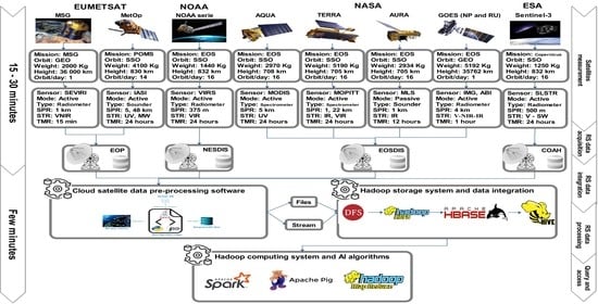
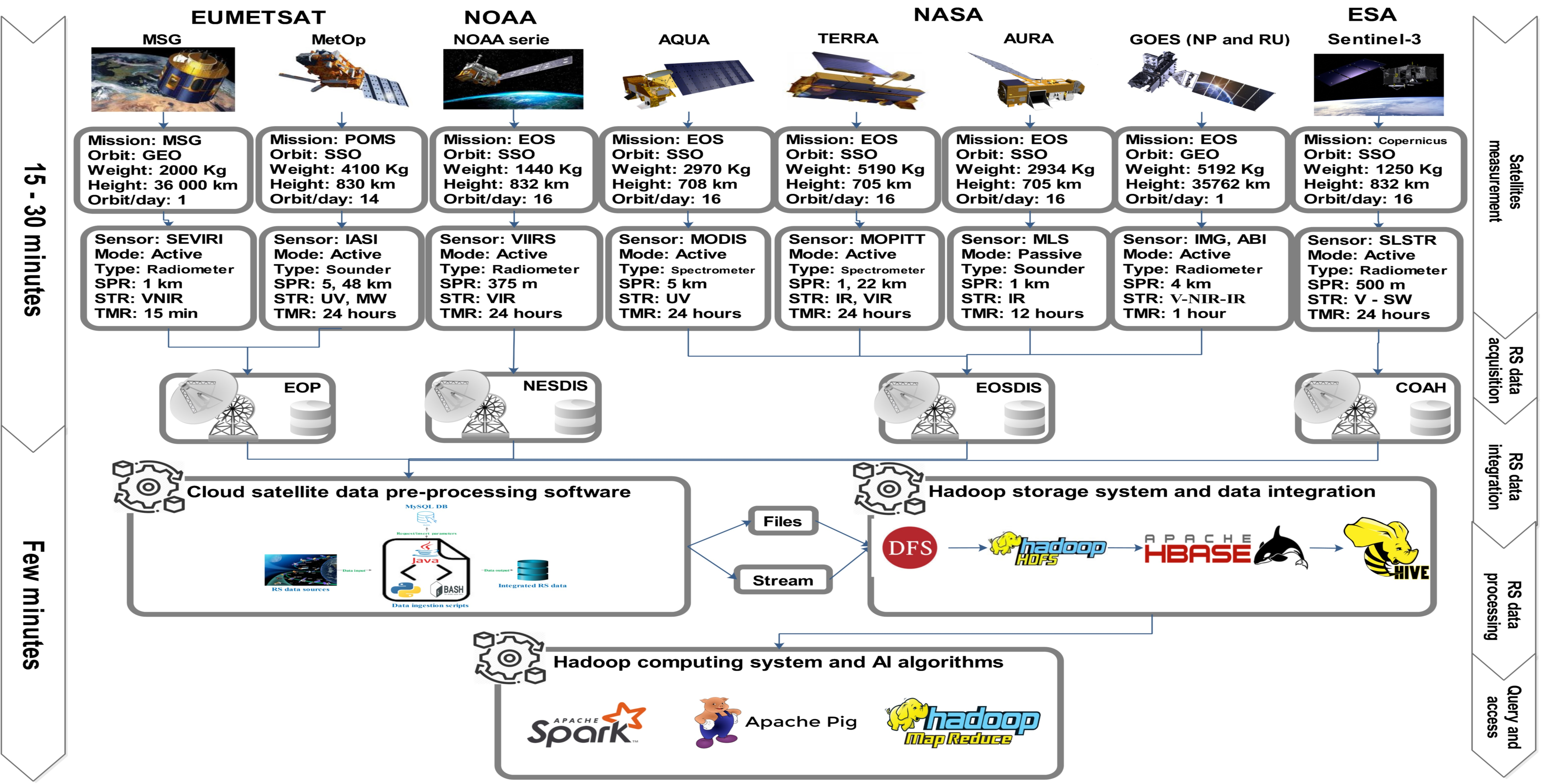
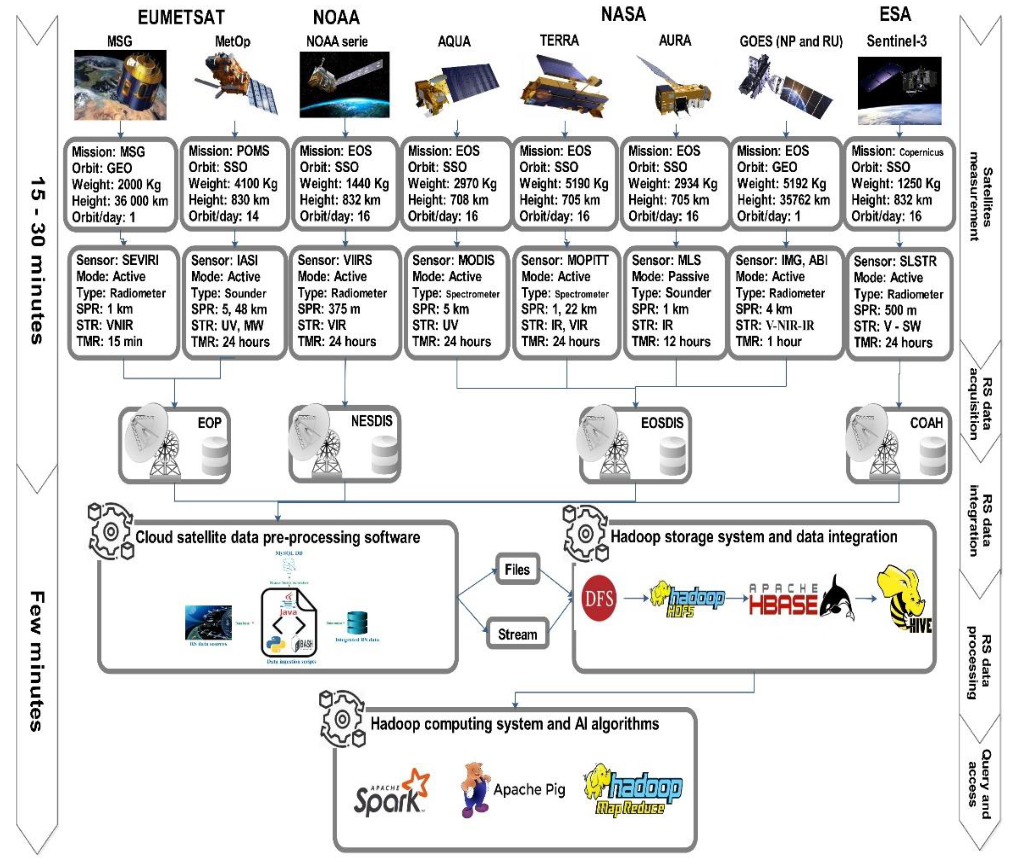
This section describes the proposed SAT-Hadoop-Processor architecture, explains Hadoop’s implementation, and shows how to include cloud computing, especially the OpenStack and parallel programming for RS data ingestion. Figure 1 illustrates the SAT-Hadoop-Processor architecture. We note the steps from RS data acquisition to the last query and access in such a schema as briefly explained in the following subsections.

3.1. Satellite Measurement and RS Data Acquisition

In this study, we gathered data from the European Organization for the Exploitation of Meteorological Satellites (EUMETSAT) via the Mediterranean Dialogue Earth Observatory (MDEO) ground station installed at the Abdelmalek Essaâdi University of Tangier in Morocco [26] and the Earth Observation Portal (EOP). Besides, we obtained RS data from the Earth Observation System Data and Information System (EOSDIS) of NASA, the Infusing Satellite Data into Environmental Applications (NESDIS) of the NOAA, and the Copernicus Open Access Hub (COAH) platform operated by the ESA. The RS data collected came from many polar satellites flying in Sun-Synchronous Orbit (SSO)—MetOp, NOAA, and Sentinel series, AQUA, TERRA, AURA, etc.—and Geostationary Earth Orbit (GEO) satellites, notably the Geostationary Operational Environmental Satellite (GOES-NP and RU) series and the Meteosat Second Generation (MSG), etc.

In our study, we acquired data from several passive and active satellite sensors [27]: Spinning Enhanced Visible and InfraRed Imager (SEVIRI), Infrared Atmospheric Sounding Interferometer (IASI), Visible Infrared Imaging Radiometer Suite (VIIRS), Atmospheric Infrared Sounder (AIRS), Moderate Resolution Imaging Spectroradiometer (MODIS), Microwave Limb Sounder (MLS), Advanced Baseline Imager (IMG), Sea and Land Surface Temperature Radiometer (SLSTR), etc. The used satellite instruments have different spatial resolutions ranging from 375 m to 5 km. and a spectral resolution diverting from microwave (MW), shortwave (SW), near-infrared (NIR), infrared (IR), visible (V), and ultraviolet (UV). Besides, the temporal resolution varies from a few minutes to a few days. Wget [28], dhusget [29], and Sentinelsat [30] Linux libraries have been used to download RSBD in NRT from the links detailed in

Table 3. RS data sources’ URLs.

Data Source	CMD	Download Link
MDEO	CMD 1	https://www.eumetsat.int/eumetcast
EOSDIS	CMD 1	https://earthdata.nasa.gov/earth-observation-data
NESDIS	CMD 1	ftp://ftp-npp.bou.class.noaa.gov
COAH	CMD 2 & 3	https://s5phub.copernicus.eu
MGS Madrid	CMD 1	https://datos.madrid.es/portal/site/egob

. The use of the commands (CMD) lines is noted as follows:

• CMD 1: wget-r-nc—accept=Extension—no-parent—dns-timeout=500-P Output path—user=Username—password=Password Link &
• CMD 2: bash dhusget.sh-d Link-u Username-p Password-m “Sentinel-5 P”-i TROPOMI-t TimeAgo (second)-T “$i”-o product-O Output path &
• CMD 3: sentinelsat-u s5pguest-p s5pguest-s StartDate-e EndDate-d—sentinel 5—producttype L2__O3____—location CityName—url “https://s5phub.copernicus.eu/dhus/”

3.2. RS Data Ingestion

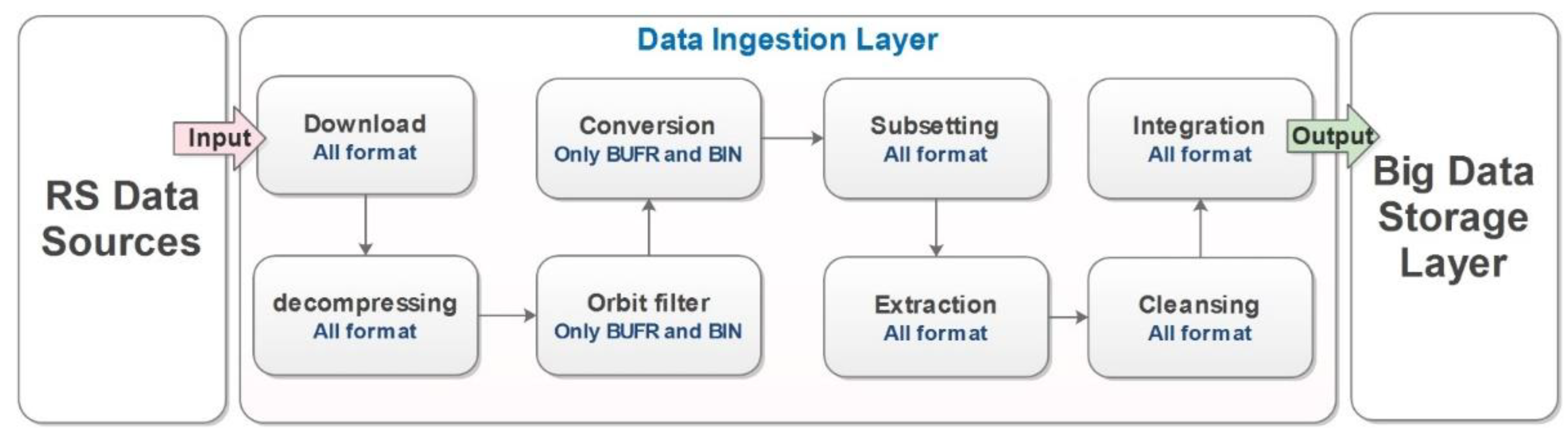
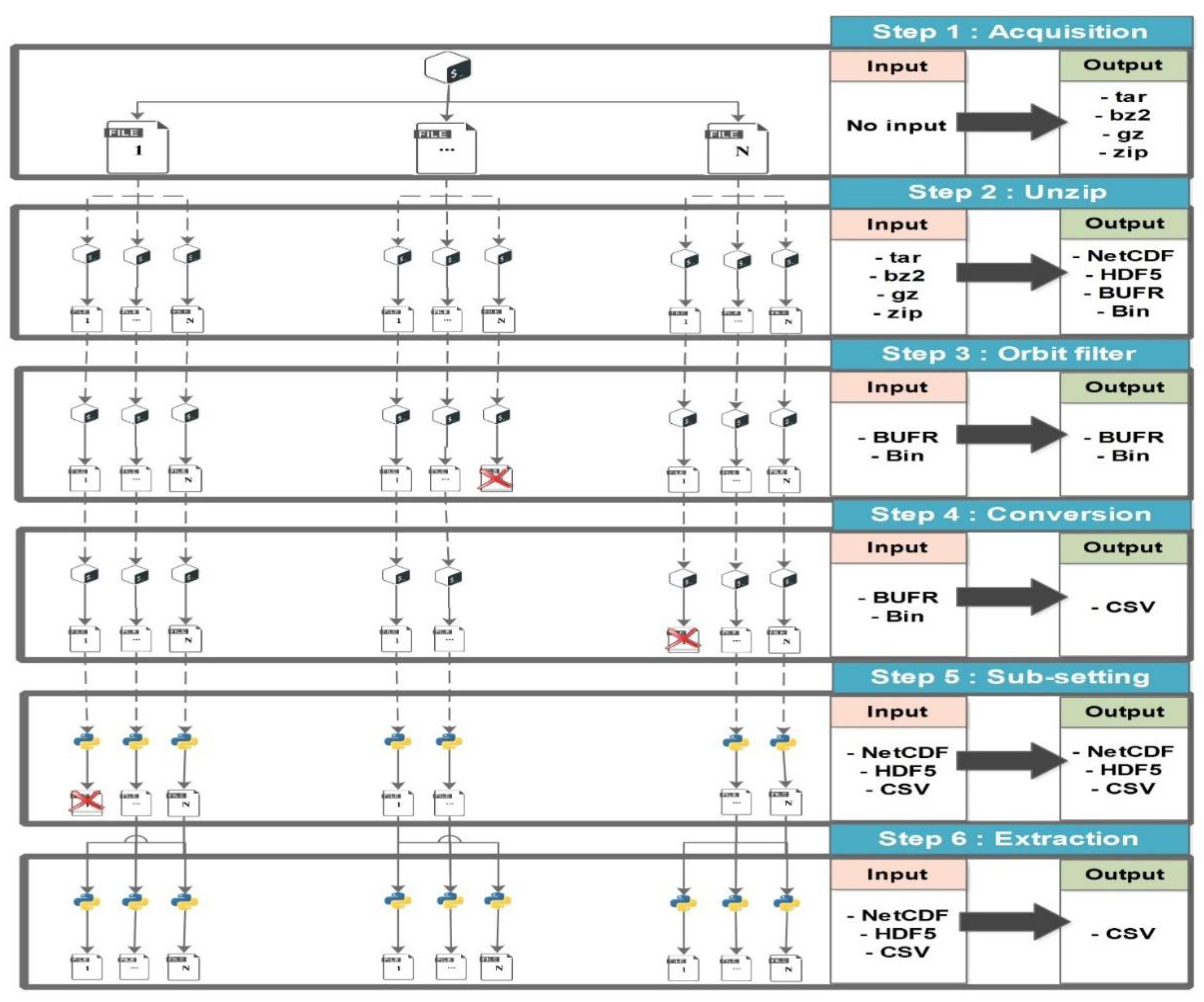
The processing chain of the RSBD takes in many challenges. First of all, satellite data are diffused into ground stations, so the big complaint is how to gather these data in NRT to keep data fresh. These data should be pre-processed to remove erroneous, inaccurate, and unneeded datasets to retain only data of interest and integrate them into a distributed and scalable storage platform. Figure 2 displays the six phases of the ingestion layer. The acquisition is the initial step in the satellite data processing.

We acquired data automatically from the sources mentioned in Section 3.1. The downloaded files were compressed from the ground station and datacenters. Therefore, the following phase decompresses satellite data automatically by a Bash script (Tar, Zip, and bz2); thus, the number of files grew 240 times, and the size increased up to 40%. Based on these results, we confirm that RS data require more storage space and become more complex for processing after the decompression step.

Commonly, the HDF5, NetCDF, BUFR, and BIN file formats are dedicated to storing RS data. These data require conversion from the scientific file format to a CSV or the Extensible Markup Language (XML) file format. We employed two Python libraries: the BUFRextract (BUFREXC) and the pybufr_ecmwf (ECMWF). Afterward, datasets are prepared to be extracted. So, the total size of data stays roughly the same after the conversion.

The downloaded data come from polar satellites flying in a Low Earth Orbit (LEO) with an altitude of 800 km and making 16 orbits daily. Thus, the processing of all data of the Earth takes more computing resources and a long execution time. We coded Python script filtering satellite data by countries using the longitude and latitude. We found that big countries, such as the USA, China, and Australia, have many files, reaching more than 700 files per day. However, the smallest state, which is Qatar, covers only about 50 files, and the data size is megabit (MB). The next step is data extraction. It permits the selection of the looked-for variables. For example, we were interested in 12 variables: temperature, humidity, pressure, wind speed, AOD, the Vertical Column Density (VCD) of trace gases, etc. The final step is the data integration into the HDFS, HBase, and Hive storage framework of Hadoop using some CMDs detailed in the Supplementary Materials File (SMF). The main algorithm in which the SAT-Hadoop-Processor was developed is as follows:

• ST is the system set of satellites of interest {st1, …, stn}.
• SS is the used satellite sensor {ss1, …, ssn}.
• P is the used satellite products {p1, …, pn}.
• F is the acquired satellite files {f1, …, Fn}.
• UF’ is the unzipped RS files {uf’1, …, uf’n}.
• CF’ is the converted RS files {cf’1, …, cf’n}.
• FF’ is the orbit filtered RS files {ff’1, …, ff’n}.
• EF’ is the extracted RS files {ef’1, …, ef’n}.
• V is the used satellite variables {v1, …, vn}.
• D is the extracted RS dataset {d1, …, dn}.
• FD’ is the filtered RS dataset {fd’1, …, fd’n}.
• CD’ is the unit converted RS dataset {cd’1, …, cd’n}.
• FD’ is the final RS dataset {fd’1, …, fd’n}.
• We can also define the main functions and threads (scripts) of processing as follows:
• T-Acquisition (): the thread of RS data acquisition.
• T-Decompression (): the thread of RS data unzipping.
• T-Conversion (): the thread of RS data conversion.
• T-Filtering (): the thread of RS data orbit filter and subset.
• T-Extraction (): the thread of RS data extraction and serialization.
• T-Integration (): the thread of RS data integration in the Hadoop.

3.3. Cloud-Distributed RS Data Ingestion

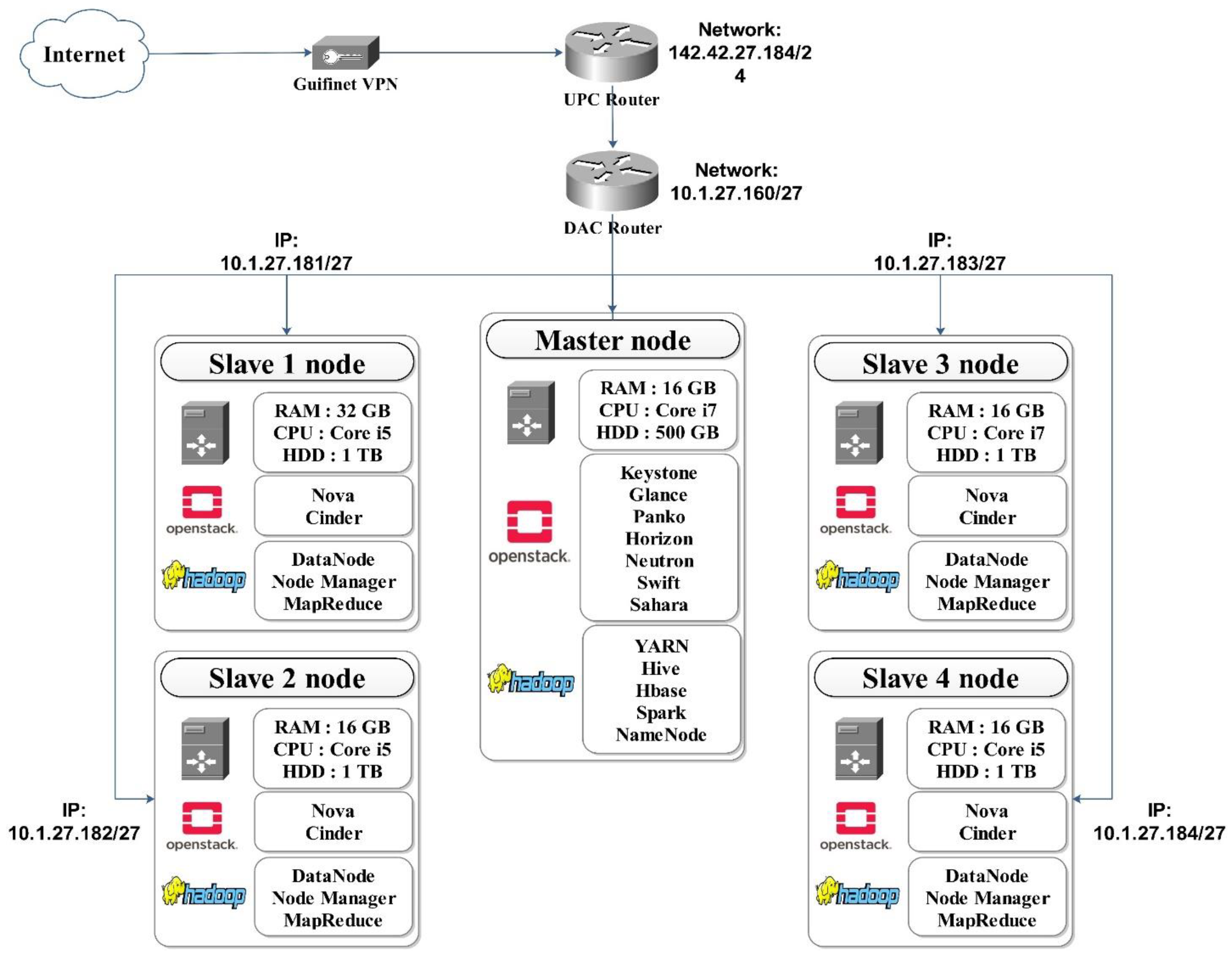
In this study, we deployed the OpenStack for a private cluster in the University Polytechnic of Catalunya (UPC). This small pool comprises one controller node, four compute, and one network node, as shown in Figure 3. All the used nodes were run with Intel(R) Core (TM) i5 or i7 Central Processing Unit (CPU)@ 2.50 GHz and 16 or 32 GB Random-Access Memory (RAM), running the Centos 7 (64 bit). All the slaves were equipped with 1 TB of the Hard Disk Drive (HDD). However, the controller was configured with 500 GB. The cluster was connected with the UPC routers. The master contains the Keystone, Glance, Panko, Horizon, Neutron, Swift, and Sahara packages. Thus, the compute nodes encompassed only the Nova and the Cinder components. Besides, Sahara allowed us to install the Hadoop tools inside the OpenStack cluster to process BD efficiently.

To create a private cloud cluster, we used the Packstack packages dedicated to Linux Centos 7. We resumed the following installation steps: network security allowance, system update, the installation of the sources, and the Packstack packages. After, the generation and the customization of the configuration file (answers_files.txt) occurs. Finally, the deployment of the installation takes about one hour. If the installation succeeds, we can access the Horizon dashboard via this link: IP_server:8080.

3.4. Parallel RS Data Ingestion

We used parallel programming libraries to optimize the ingestion process execution time, notably, the Linux Background Processing (LBP), GNU Parallel, Python parallel, and the multi-threads of Java. The LPB is a process that is started from a shell and then executes independently using this symbol (&) after the CMD; the same terminal will be instantly available to run further CMDs.

The GNU Parallel is used to compile and run CMDs parallel to the same CMD with several arguments, whether filenames, usernames, etc. It provides shorthand references to many of the most common operations, mainly the input lines, sources, etc. It can also replace xargs or feed CMDs from its input sources to several Bash instances. CMD 4 shows that the parallel execution exploits 95% of the hardware in the subset script using the GNU parallel library: CMD 4: Bash subset_script.sh | parallel—load 95%—noswap ‘{}.’

The Python parallel is a library that simultaneously executes several processes or scripts in multiple processors in the same computer or cluster. It is intended to decrease and optimize the total processing time. CMD 5 illustrates how to execute many functions simultaneously in Python using the Python parallel library: CMD 5: Th = threading.Thread(Functions); Th.start(); Th.join(). Java Multithreading is a Java option that permits parallel execution of two or more program parts to maximize hardware capacities.

Figure 4 summarizes the input format and the output format of the six steps of pre-processing. The ingestion layer was conceived for RSBD pre-processing; it can hold a colossal input data volume and extract the information needed from satellite data. As illustrated in Figure 1, this ingestion layer was developed by some detached and interconnected scripts: Java, Python, and Bash are the primary programming languages employed in coding.

The Bash was used to connect automatically, download RSBD from various sources, and manage many files. Python scripts are mostly used to extract, serialize, and deserialize the final output datasets. Lastly, the Java application aggregates, calls, run all the established scripts and connects with MySQL DB to select parameters and insert benchmarking monitoring results.

The mechanism of how the layer functions is that in parallel (LPB), the RSBD is downloaded from several links using Wget. A Bash script decompresses in parallel (GNU parallel) the collected data using the Tar, Unzip, and Gunzip libraries. Afterward, a Bash script parallel (LBP) filters the data. Another Bash script converts in parallel (GNU parallel) the BUFR, Bin, and GRIB data to the CSV format using the BUFRextract (BUFREXC) and the pybufr_ecmwf (ECMWF). The converted data are subset and extracted in parallel (Python parallel) using the h5py and Pyhdf libraries. Finally, the final CSV output is loaded and integrated into the Hadoop system.

3.5. RS Data Integration and Storage: Hadoop Framework

In this section, we explain how to create a Hadoop cluster for RS data integration and storage. In our work, we worked with the HortonWorks distribution launched in 2011. This version’s components are open source and licensed from Apache to adopt the Apache Hadoop platform [31]. HortonWorks is a significant Hadoop contributor, and its economic model is not to sell a license but to support sales and training exclusively. This distribution is most consistent with Apache’s Hadoop platform. More configuration details can be found in the following link: https://www.techrunnr.com/how-to-install-ambari-in-centos-7-using-mysql/ (accessed on 7 November 2021). After the successful installation, deployment, and configuration, we can access the Ambari dashboard via the link IP-Server:8080 containing all the metrics and the cluster’s customization tools.

This study integrated and stored the pre-processed RSBD inside a Distributed File System (DFS) in a scalable way across a distributed Hadoop cluster. DFS is a virtual file system that affords data nodes’ heterogeneity in various centers [32]. Thus, the DFS provides a standard interface for applications to manage data on different nodes that use the other OS. DFS can retain a replica of data further than one node; thus, the image is preserved and restored if needed in the event of a fault. DFS is scalable, where the number of compute nodes can be amplified to optimize the processing. 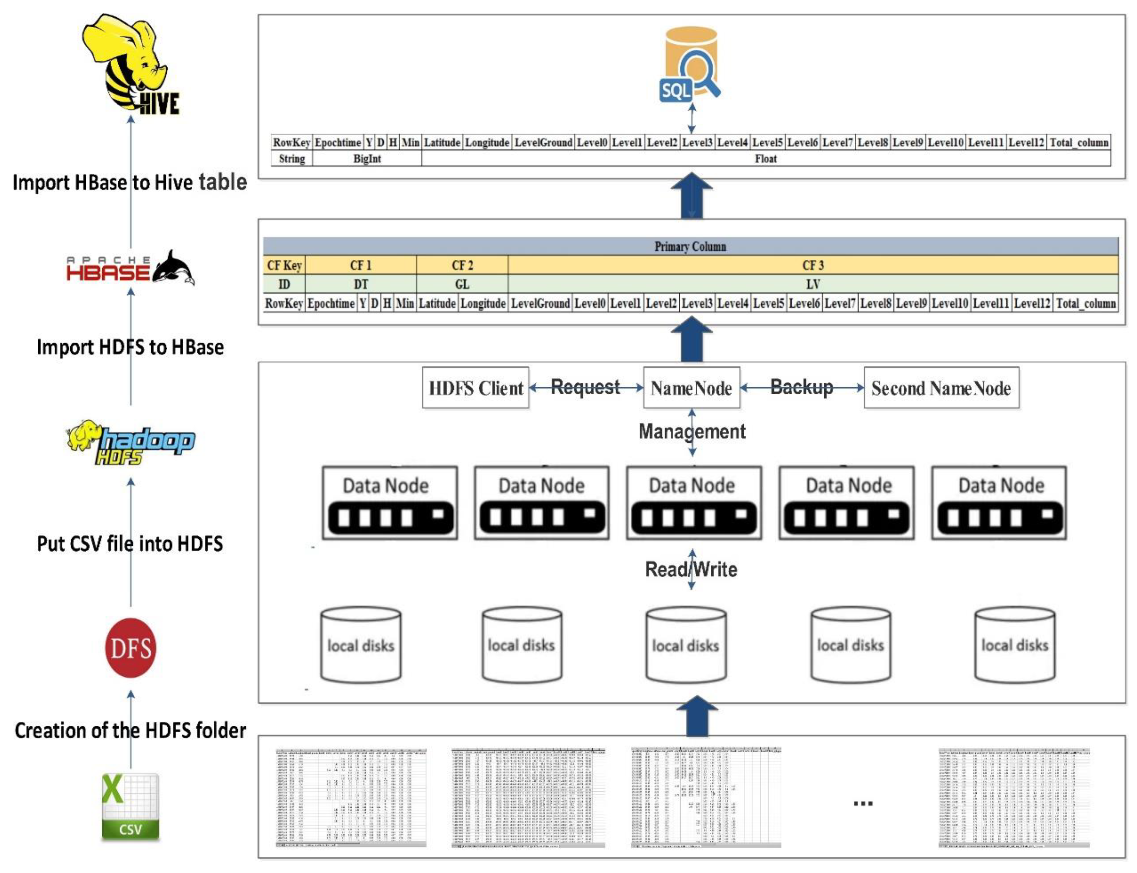Figure 5 shows the general paradigm to integrate and store pre-processed files stored in a CSV file to DSF, HDFS, HBase, and the Hive table.

The first step makes the DFS and HDFS folder for storing, yielding access to the folder, copying the CSV file to HDFS, before importing the HDFS to HBase based on the primary column and the Column Family (CF), and lastly, generating an external Hive table for the HBase table. Accordingly, the CSV file is stored in Hadoop, which can be requested and retrieved using HiveQL language only and is comparable to the SQL language queries.

3.5.1. The Exportation of RS Data into the HDFS

HDFS is intended mainly for big datasets and high availability. It is also an independent framework implemented in Java [32]. Compared to other DFS, it is specified that the performance is different in design, and HDFS is the individual DFS with automatic load balancing [33]. In this investigation, we are looking forward to storing the integrated data from the ingestion layer’s output to an HDFS. It is an excellent tool that can hold a colossal volume of data, afford easier access, and performs data replication to prevent data losses in the case of failure or damage [34]. Furthermore, the HDFS facilitates parallel data processing, and the chief master/slave is the topology [35] (see Supplementary Material File).

3.5.2. The Integration of RS Data in the HBase

HBase is a column-oriented key/value storage system made to run on the upper of the HDFS. The Apache Software Foundation accomplishes its development. HBase became a top-level Apache project in 2010. It is designed to manage significant table operations and request rates (billions of rows and millions of columns) and scale-out parallelly in distributed computing clusters [36]. HBase is recognized for offering robust data consistency on reads and writes, which differentiates it from other NoSQL databases [37]. It uses the architecture of master nodes to handle region servers that distribute and process parts of data tables. HBase is a chunk of a long list of Apache Hadoop frameworks that embrace Hive, Pig, and Zookeeper tools. HBase is typically coded using Java, not SQL. The most common Filesystem used with HBase is HDFS [38]. Nevertheless, you are not limited to HDFS because the Filesystem used by HBase has a pluggable architecture and can replace HDFS with any other supported system. In effect, you could also implement your Filesystem (see Supplementary Material File).

3.5.3. The Storage of the RS Data in Hive

Hive is an open-source data warehousing tool made on top of Hadoop. It was open-sourced in August 2008, and since then, it has been explored by many Hadoop users for their data processing requests. Hive executes queries in the SQL declarative language, HiveQL, which are performed in MR jobs using Hadoop [39]. Furthermore, HiveQL allows users to plug custom MR code into queries. The language contains a type system supporting tables containing native types, such as arrays and maps. The HiveQL includes a subgroup of SQL and some extensions that we have found useful in our environment. Standard SQL features are similar to clause subqueries, various types of joins: joins, cartesian products, grouping, aggregations, union all, create table as select, and several useful functions on primitive and sophisticated types make the language very analogous to SQL. Hive also takes in a system catalog, the Metastore, containing schemas and statistics useful for data exploration, query optimization, and compilation [40].

Hadoop is not easy for end-users who are not familiar with MR. End-users must write MR scripts for simple tasks, such as calculating raw counts or averages. Hadoop requires popular query languages’ expressiveness, particularly SQL, and thus users spend a long-time coding program for even simple algorithms. We frequently run thousands of Hadoop/Hive cluster jobs for various applications, from simple summarization to machine learning algorithms. Hive serializes and deserializes using a java interface offered by the user. Thus, custom data formats can be taken and queried (see Supplementary Material File).

4. Experiment and Results

This section describes the experiment directed according to the description of the case study. Firstly, we detail the used hardware and RSBD input for the investigation: mainly the launched instances for pre-processing and the input size of the pre-processed RS data. It also shows the pre-processing software’s statistical results, particularly the output data, the execution time, and benchmarking. Besides, it illustrates how to access and explore the final datasets stored in the Hadoop storage layer.

4.1. Instances and VMs

Table 4. The configuration of the used VMs.

Instance Type	Instance (VM)	VCPU	RAM	Storage
Private (UPC)	Instance 1	7	16	HDD
Private (UPC)	Instance 2	8	32	HDD
Public (AWS)	Instance 3	16	64	SSD
Public (AWS)	Instance 4	32	128	SSD

shows the four VMs launched for RSBD pre-processing. Thus, we created instances 1 and 2 using the local cluster of the UPC equipped with OpenStack. On the other hand, we allocated instances 3 and 4 using the Elastic Compute Cloud (EC2) of the Amazon Web Services (AWS) to obtain more computing capacities for testing.

This paper acquired NRT data from five sources: the MDEO, NASA, NOAA, ESA, and some Meteorological Ground Station (MGS). The data were measured with around 25 satellite sensors and more than 60 ground sensors. The collected data were transmitted through downlink channels, providing about 50 products. Moreover, the data were stored in a scientific file format, such as NetCDF, HDF5, BUFR, and GRIB. The total daily volume of data sums up 50 GB, and the velocity reaches more than 40,000 files per day. The acquired data’s latency averages between one minute and three hours, as shown in

Table 5. The specifications of the daily input data.

Organizations	Sensors	Products	File Format	Size/ Day (GB)	Velocity/ Day	Latency (Minutes)
MDEO	8	27	NetCDF,	10	20,000	1–35
NASA	8	14	HDF5,	12	7000	40–140
NOAA	6	6	BUFR,	14	8000	60–180
ESA	3	5	GRIB,	17	150	120–180
MGS	61	7	Bin	1	100	1–10

. The total number of plots (a single measurement of a variable in a specific time and location in the map) in Morocco 24 h sumps up 10 million datasets.

4.2. Benchmarking

The experiments were run on the created VM running Debian GNU/Linux 10 (64 bit). During the execution of the developed SAT-Hadoop–Processor software, we monitored some benchmarking using the CMD 6: time-f “%e_%P_%M_%S

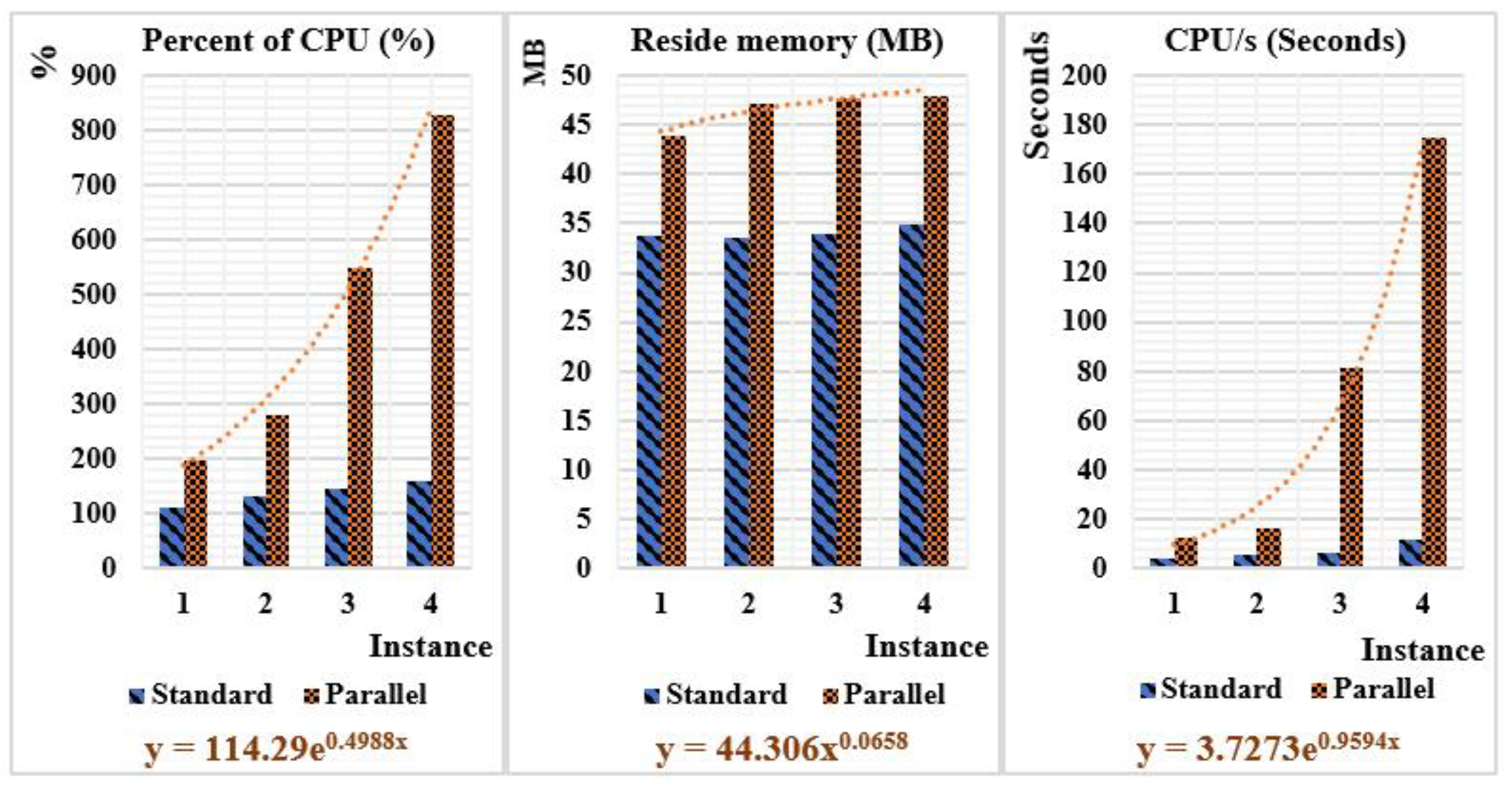
Figure 6 shows that in parallel mode, the percent of CPU, the maximum reside memory, and the CPU/s increase significantly when the VM size grows because the software executes as many scripts simultaneously. Still, in standard mode, the software does not yield totally from the hardware capacity available in the cluster. Accordingly, we assumed that the parallel execution maximizes the employment of the hardware capacities to improve the execution time.

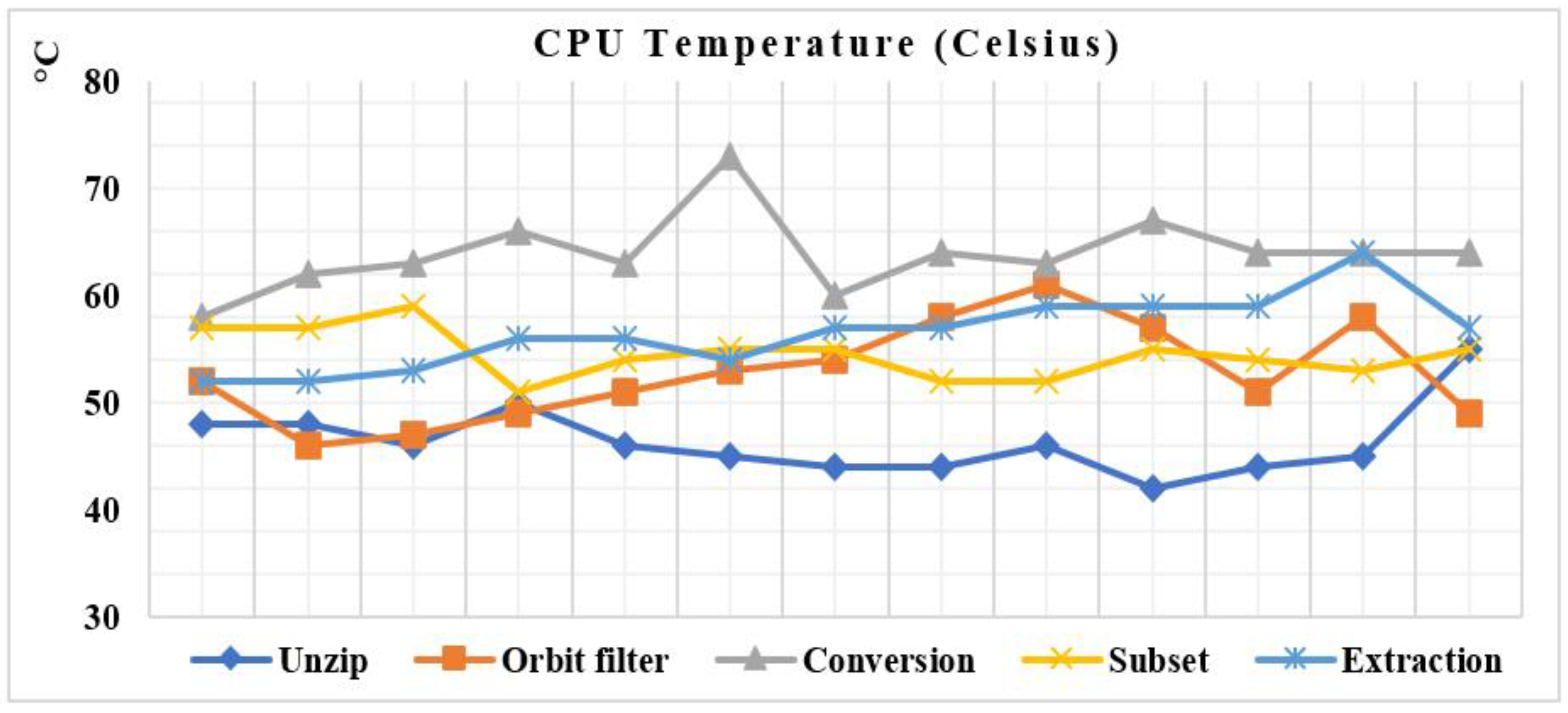
Figure 7 shows the mean temperature of the CPU during all the pre-processing steps. Thus, the temperature ranges from 40 to 75 °C. It depends on the number of inputs, output files, the algorithm’s complexity, and the operation’s nature (reading, writing, calculating, networking, and so on). We note that the CPU’s temperature is moderate, about 55 °C, during the decompression and the orbit filter steps because these two operations manage files in the HDD (moving, deleting, etc.). However, the CPU’s temperature is high, around 65 °C, during the conversion, subset, and extraction because these scripts include many loops and computation instructions, so they consume further CPU.

4.3. RS Data Output

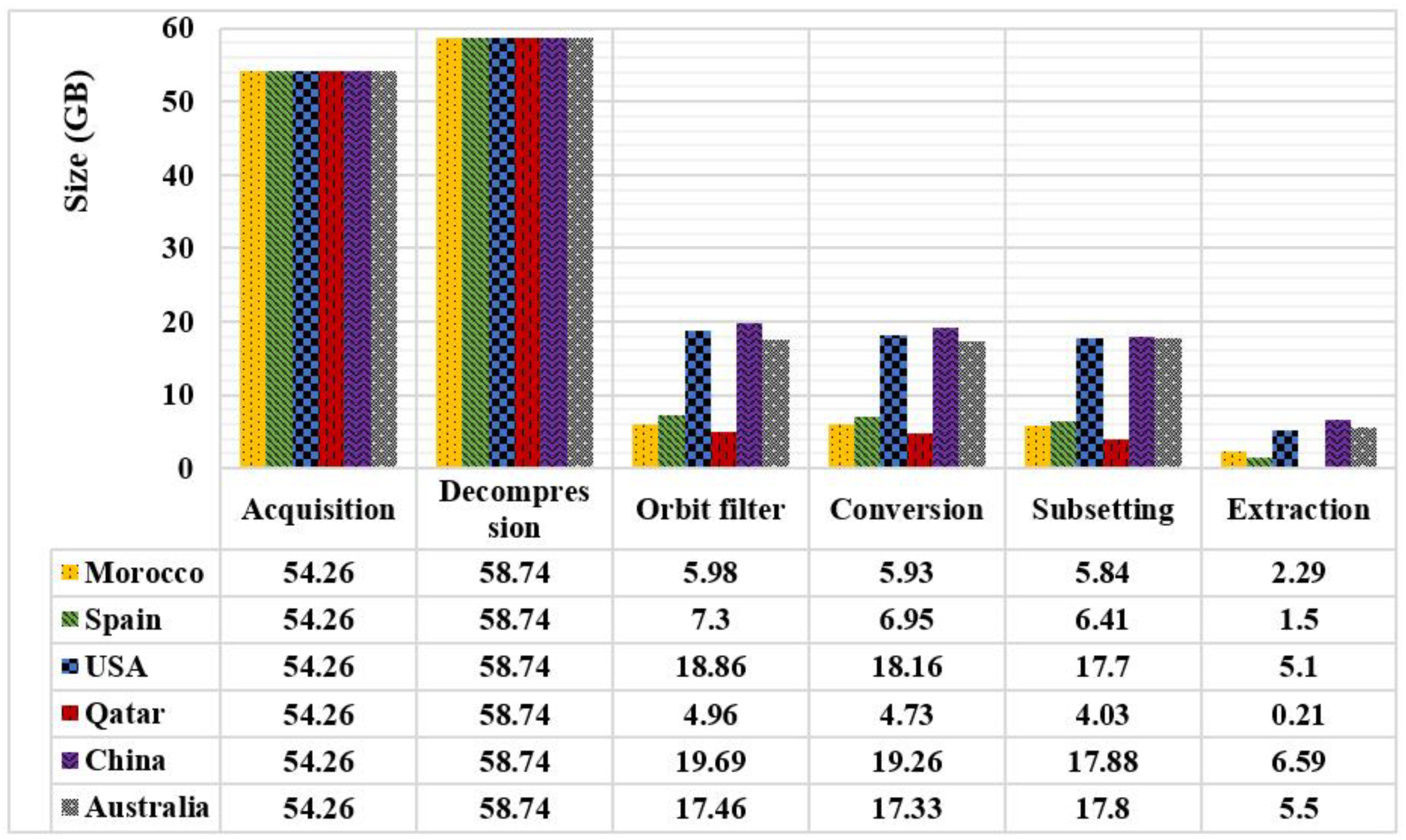
The ingestion layer achieved an automatic download, decompression, filter, conversion, subset, and extraction efficiency. Hence, as shown in Figure 8, we note that the total daily size collected as input is around 50 GB. A 10% growth occurred after the decompression because the ground station compresses RS data to smooth transmission. After the conversion step, the total size remains the same size. Still, after the subset process, data decreases meaningfully due to the exclusion of unnecessary data. Globally, this ingestion layer allows us to increase the storage space by 86%. Thus, the final CSV files’ total size is between 1 and 6 GB depending on the studied country’s surface area. Therefore, this relevance could be considered as a partial solution to the satellite data’s perversity.

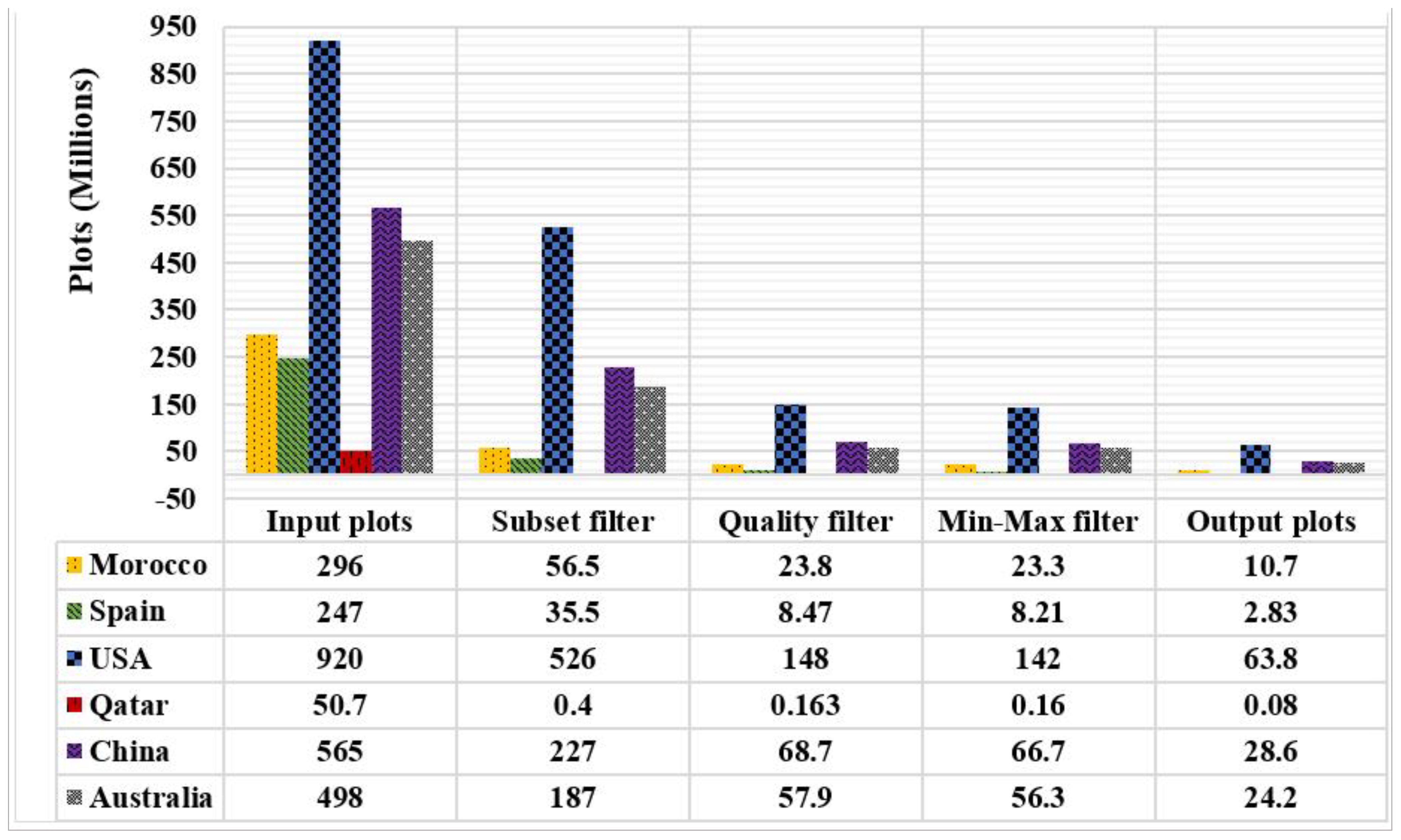
The extraction is the final and significant stage of the ingestion layer. Figure 9 describes the daily total number of plots of the six countries. After the subset, we note that the sum of plots decreases exponentially to retain only datasets covering the countries’ zone of interest. The quality, minimum, and maximum filter eliminate about 20% of inaccurate and erroneous datasets. Lastly, the refined and final datasets (rows) were stored in associated CSV output files loaded and imported into an HDFS.

Consequently, the extraction also diminishes the number of inaccurate and unneeded datasets by up to 20%. The daily total number averages between thousands to millions of plots conditional to the studied country’s surface area. This result confidently applies an efficient Extract Transform Load (ETL) process to the RSBD and adapts it for integration into a Hadoop environment.

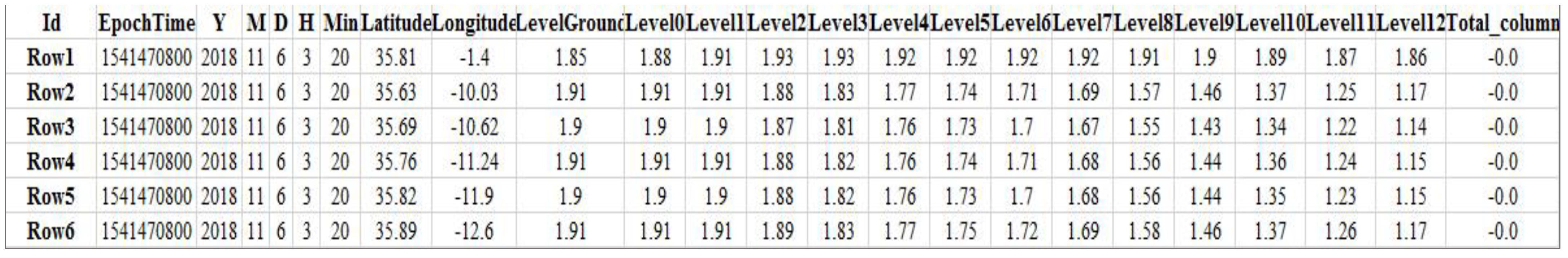
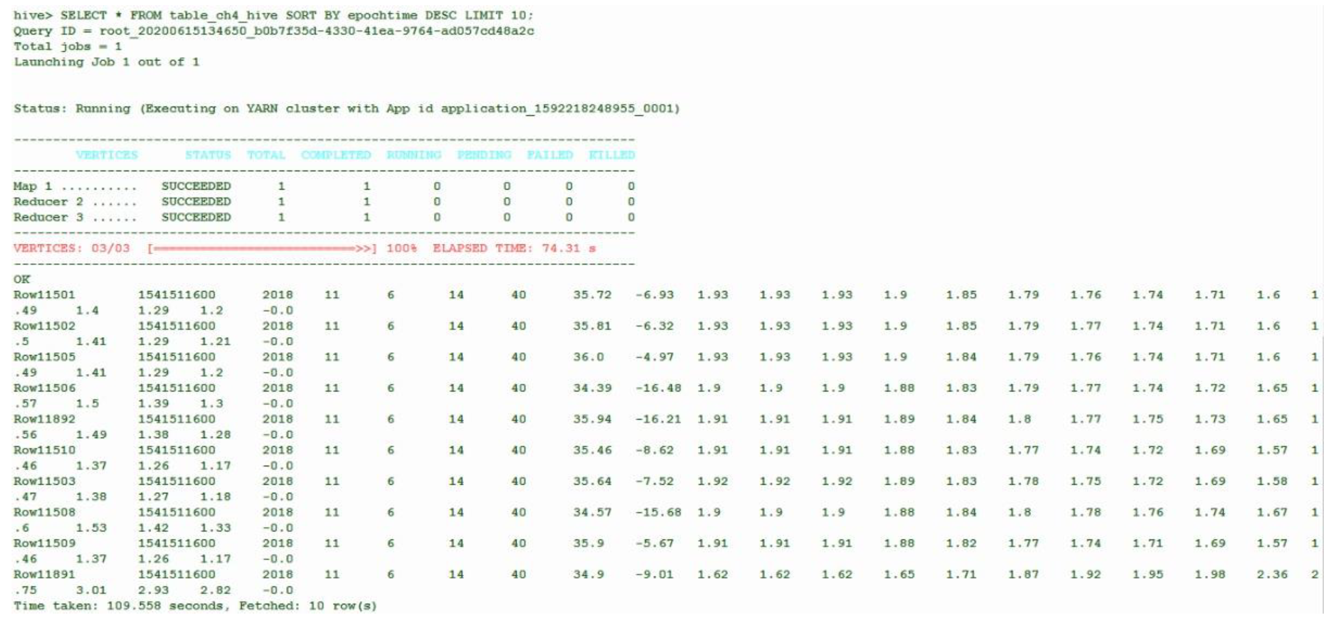
The ingestion layer results in several CSV files as outputs with a unified schema, storing datasets of several variables for each satellite, channel, and product. A final CSV file contains 24 columns: Id of rows useful to distinguish it, Epoch Time, Year, Month, Day, Min, Latitude, Longitude, and 12 atmospheric levels with an altitude between 0 and 8 km (middle Troposphere). Figure 10 shows a snapshot of the first six rows of the CSV output of the VCD of CH₄ in Morocco.

4.4. RS Data Queries Access and Interpretation: HiveQL and MR

This study integrated the output CSV files in the HDFS. This helps to handle RS data’s enormous volume, variety, velocity, and value. HDFS supports arranging, storing, and cleaning the data, making it suitable for analyzing massive parallel processing.

HDFS is based on a cluster with independent machines in which every node performs its job using its resources. This will help to attach different computers with different OS and configurations. Besides, integrating the pre-processed data in HDFS will automatically stripe and run-on commodity hardware, which does not need a very high-end server with a large memory and processing processor. Storing the pre-processed RS data does not require large clusters to be built. We kept on adding nodes. We employed HDFS to store and access the refined easily and to generate value from RS data.

Hadoop can competently process terabytes of data in a few minutes and petabytes in hours using MR. Importing the ingested RS data in HDFS is also replicated in other nodes in the cluster, which means an alternative copy exists for use in the incident of failure. Importing some GB of data inside the used Hadoop cluster takes approximately a few minutes, and the visualization only a few seconds.

We also stored the HDFS files inside the HBase system to aggregate and analyze billions of rows of the refined RS datasets. Furthermore, compared to traditional relational models, the data could be shared with other users as end-users quickly and with a small amount of reading and writing time. Storing the output data in HBase also helps to perform online and NRT analytical operations. The importation of massive data from HDFS to HBase involves only a few minutes. HBase does not support SQL requests in contracts and shows a large memory and high CPU performance to process massive inputs and data outputs. The system involves fewer task slots per node to allocate HBase CPU requirements in a shared cluster environment.

This study stored the pre-processed RS data in Hive external tables, as shown in Figure 11. Hive helps simplify working with billions of rows, using the HiveQL, which is much closer to SQL than Pig and has less trial and error than Pig. Hive also analyzes the massive RS data without strong java programming skills for writing MR programs to retrieve data from the Hadoop system. Importing some GB of data inside the Hive external table takes approximately a few minutes, and the visualization only takes a few seconds [19].

4.5. The Optimization of the Total Execution Time

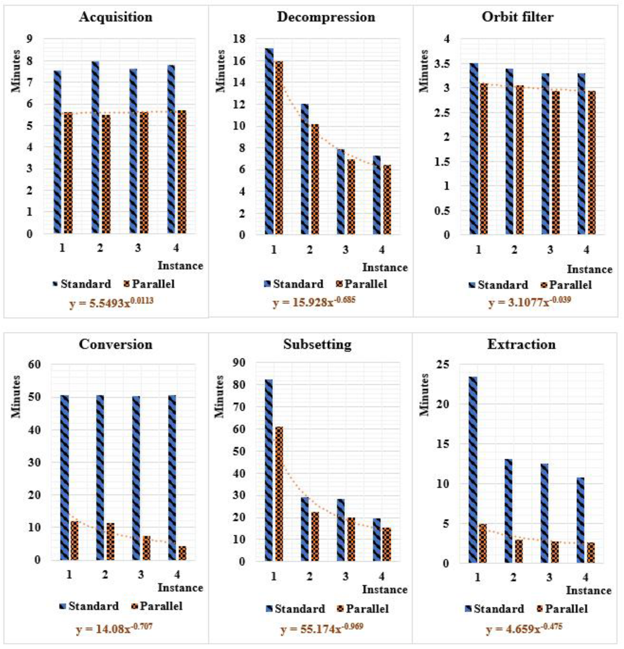
Our experiment ran the ingestion software in four different VMs, as detailed in Table 4, with an Internet bandwidth of 1 GB/s. Commonly, the pre-processing of the RSBD takes a long execution time. From Figure 12, we remark that the download phase took approximately eight minutes in standard mode and around six minutes when the parallel tools were applied. This time could be optimized more by speeding up the Internet bandwidth or/and switching the Internet Protocol (IP) from the Transmission Control Protocol (TCP) to the User Datagram Protocol (UDP).

The decompressing and the orbit filter execution time requires 20 min in standard mode and only about 10 min in parallel. The conversion is the lengthiest process, reaching about 50 min in standard and less than 10 min with a parallel algorithm. The subset needs more than an hour in standard; however, it requires only 15 min parallelly. In conclusion, the extraction script takes an average of 20 min. In contrast, it takes only three minutes with the parallel approach.

The developed scripts are optimized by reducing database connections, such as selections and insertion requests; thus, the network traffic economizes. Removing unused loops by breaking the loops by conditions is also essential to reduce CPU and RAM consumption. Besides, discarding the collections lists, arrays, and vectors after each file processing reduce RAM utilization.

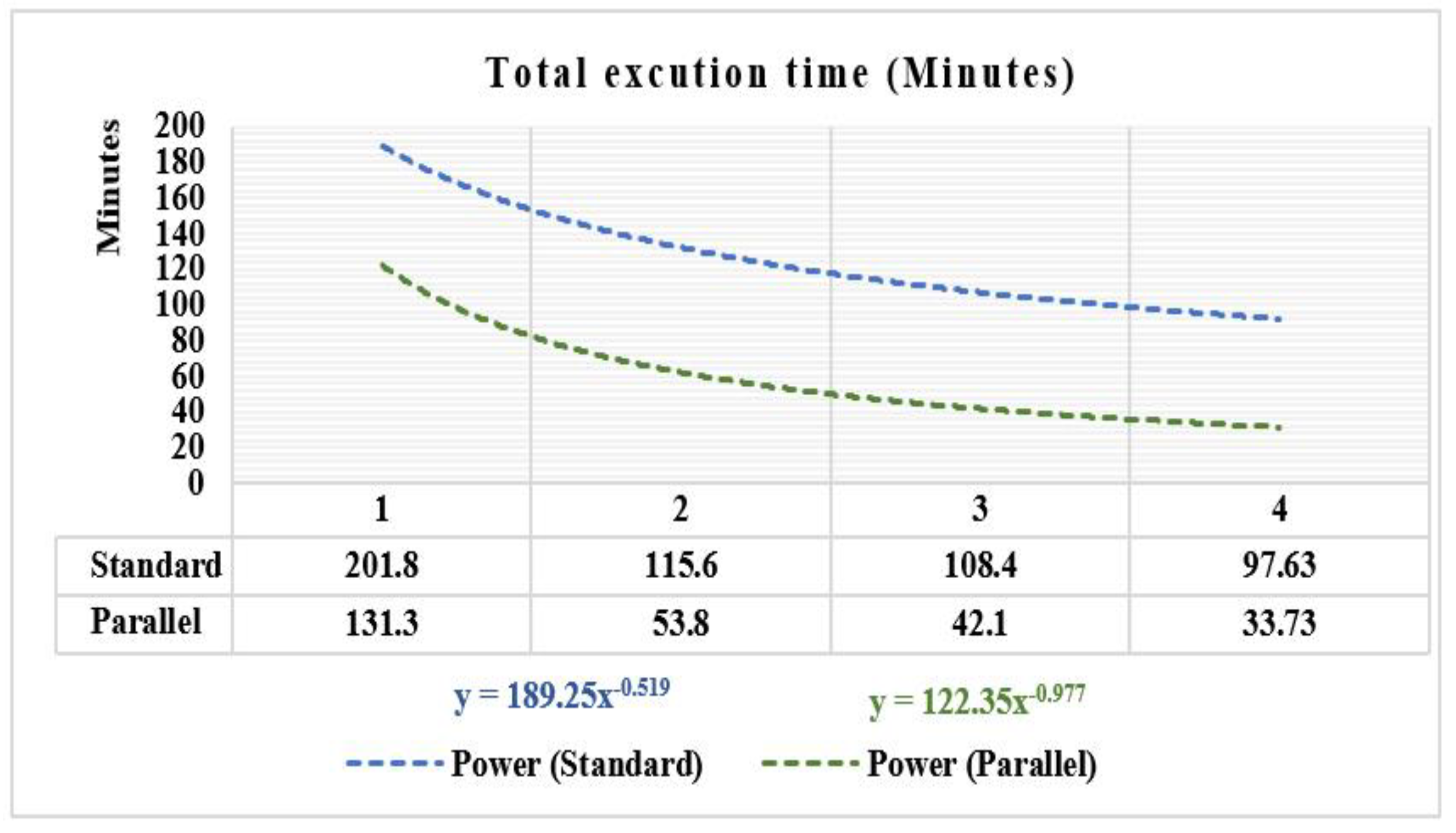
Scaling the input and output operations by only filtering datasets of interest accelerates the execution time and makes more free memory available. Finally, reducing the number of reads and write processes surely adjusts the HDD and CPU performance. In this testing, and according to Figure 13, the total pre-processing time of 55 GB of RSBD takes more than nine hours in the standard mode Before Optimization (BO). However, it requires less than four hours in a traditional approach and within an optimized code. On the other hand, we pre-processed the same input size within an optimized code and in parallel in only 34 min. Accordingly, optimizing the code and integrating cloud and parallel programming techniques optimized the total execution time by 90%. Thus, this number could be reduced more using the power function “y” when the instance capacities (VCPU, RAM, HDD) are larger, such as a super-computer. The processing speed-up will grow when the cluster capacity is extended by adding extra VMs, reaching a plateau equal to a speed-up-max. The speed-up-max = 600/SFET, where SFET is the Single File Execution Time. In our study, the average SFET is 5 min; thus, the speed-up-max is 120 times based on the power equation shown in Figure 13 with the green color. It is worth mentioning that the speed-up factor will reach a plateau after a certain number of VMs due to the overhead in communications. The maximum number of VMs used to reach a plateau is roughly 27 VMs.

5. Comparison with Related Works

Table 6. Comparison with related works.

Feature/Study	SAT-Hadoop- Processor	SAT-ETL-Integrator [21]	[16]	[17]	[18]	[19]
Input format	NetCDF, HDF5, BUFR, GRIB, BIN		HDF5	Images	Images	Stream
Sources (Sensors)	25		1	1	1	1
Size	55 GB		50 MB	687 GB	9.5 GB	11 TB
Processing mode	Batch		Batch	Batch	Batch	Streaming
Architecture	Distributed	Single	Distributed	Distributed	Distributed	Distributed
Technologies/Tools	ETL, Hadoop	ETL	Hadoop	Hadoop	Hadoop	Hadoop
Cloud technology	OpenStack	No	No	Yes	Yes	No
Parallel computing	Yes	No	No	Yes	Yes	Yes
Languages	Java, Python, Bash		MPI	MR, Spark	MR, Spark	MR, Spark
Execution time	~30 min	~9 h	~10 min	Few hours	16 min	~135 h
Used RAM (GB)	128	16	-	576	160	160
Used CPU (Cores)	32	5	-	288	80	80
Output type	CSV	CSV	Stream	Raw data	Images	Image

compares our proposal and other related works focusing on applying RS techniques for environmental application. Please note that cells with (-) are missing the exact information. Most cited papers use scientific file formats, notably the NetCDF, HDF5, BUFR, data stream, or images regarding the input type. Instead, most of the presented studies collected data either from satellite sensors or the MGS. In contrast, in our study, we acquired data from both sources to have strong input data. Consequently, we obtained a combined output product. The streaming processing velocity sums up to millions of datasets per day, though, in batch processing, the speed is lower.

Concerning data processing, some studies adopted batch and other stream processing. Thus, our collected data are stored and then pre-processed and integrated inside the Hadoop, so we used the batch processing paradigm. We found that Python and Java are most commonly used in all the studies regarding the development language. The majority of the approaches were executed in a distributed platform, especially Hadoop. Regarding the benchmarking, we also note that streaming processing solutions take a brief execution time: less than one minute with low RAM and CPU ingesting. However, batch processing necessitates a robust cluster of processing.

Comparing this study to the SAT-ETL-Integrator software [21], we confirm that the two software have the same RS data input and output specifications. However, they differ in their processing architecture. We developed the SAT-ETL-Integrator software to pre-process RSBD in a single machine. However, with the SAT-Hadoop-Processor software, we optimized the code and integrated the cloud computing technology using parallel computing. Finally, the final result will be integrated into the Hadoop environment. Therefore, the new solution is upgraded to support parallel processing and the Hadoop framework.

The comparison of the SAT-Hadoop-Processor with [15,16] shows that they all implement distributed, cloud, Hadoop, and MR tools for scalable RSBD processing. Still, they differ in their input data format, architecture, and output. Our advanced solution has some advantages, notably the various inputs as scientific file formats provided from various satellite sensors, except optical ones providing images with pixels. The SAT-Hadoop-Processor can be customized to any EO application easily thanks to its ETL algorithm. This is not the case with other software.

6. Discussion

We suggest that our method allows complex RSBD in NRT to be dealt with. The SAT-Hadoop-Processor acquires data from multiple series of satellites and sensors automatically. It rapidly pre-processes data, keeps only relevant datasets, and finally serializes the refined output in CSV or stream, which could be consumed directly by other third-party applications or integrated into Hadoop for extra massive calculation and analysis.

We also incorporated cloud and parallel technologies to optimize the execution time by maximizing the hardware capacities. Accordingly, the developed software reduced the total execution time by 20-fold. We also integrated the ingested RSBD in Hadoop and made it compatible with HDFS, HBase, and Hive to facilitate storage and processing using MR and Spark’s pioneer tools.

The preliminary experimental results show the significant performance of the SAT-Hadoop-Processor as a promising prototype for RSBD processing. We can conclude that we successfully contributed to NRT RS data pre-processing and integration. The SAT-Hadoop-Processor is flexible software supporting several RS data input formats. It can also be customized with many EO applications, notably AP supervision, natural hazard detection [41], etc.

7. Conclusions

Currently, many environmental issues affect the equilibrium and the safety of the globe, especially AP and climate change. Thus, RS techniques play an indispensable role in AQ monitoring and climate change supervision. Although, data collected by satellite sensors are tricky, have a large size, and have high velocity. Accordingly, the RS data are BD according to the eight V salient (8Vs) of BD. Such data processing is very challenging and exceeds the capacity of current systems and architectures.

For this aim, we proposed the SAT-Hadoop-Processor software, which pre-processes a huge volume of RS data from various satellites and sensors with diverse configurations. The developed software works as an ETL, allowing practical pre-processing of satellite data, including a daily storage improvement of 86% and an RS data cleansing of up to 20%. Besides, this software is compatible with parallel processing in a cloud platform, such as IaaS. The parallel running mode optimized the execution period 20 times. This gain can be amplified by adding more hardware capacities to the cluster. As a result, the developed solution enables NRT RSBD pre-processing to preserve its freshness. Finally, the established solution integrated the Hadoop framework’s ingested data for extra processing and analysis using MR and Spark tools.

In subsequent work, we aim to work in the following directions. First, we plan to optimize the SAT-Hadoop-Processor to support satellite images (pixels) from optical sensors onboard Landsat and Sentinel. In addition, we hope to apply and test this software on different EO applications, such as natural hazard prediction, vegetation, and climate change monitoring. As a perspective, we also want to develop smart AI algorithms based on MR, allowing RSBD cleaning, interpolating, fusing, and validating. Applying some meteorological models for data prediction to help decision-makers is also an interesting work to conduct.