
Forklift Tracking: Industry 4.0 Implementation in Large-Scale Warehouses through UWB Sensor Fusion


Abstract
:1. Introduction
2. UWB Forklift Localization Method
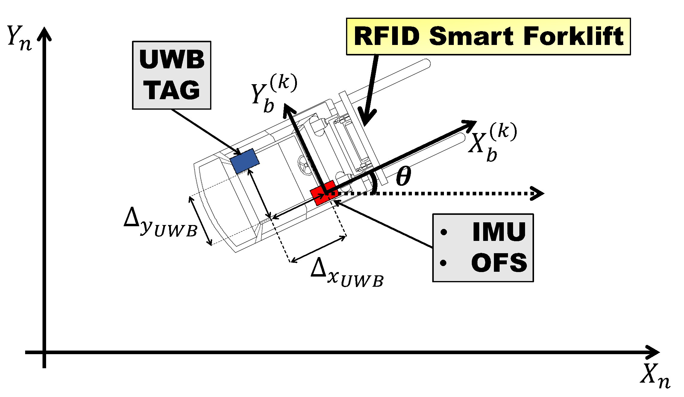
2.1. Forklift Motion Model
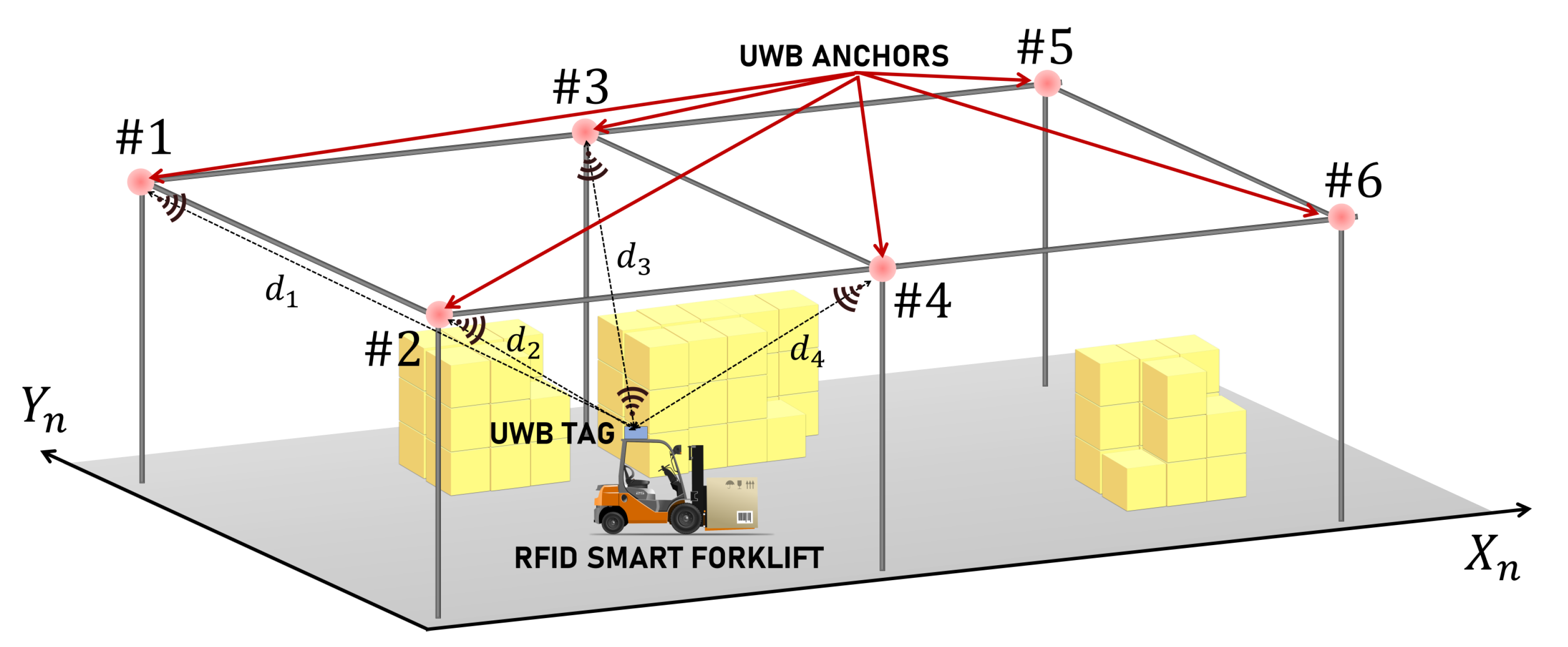
2.2. UWB Positioning
3. Numerical Analysis
3.1. Effect of Forklift Speed
3.2. Effect of Initial Uncertainty
4. Experimental Analysis
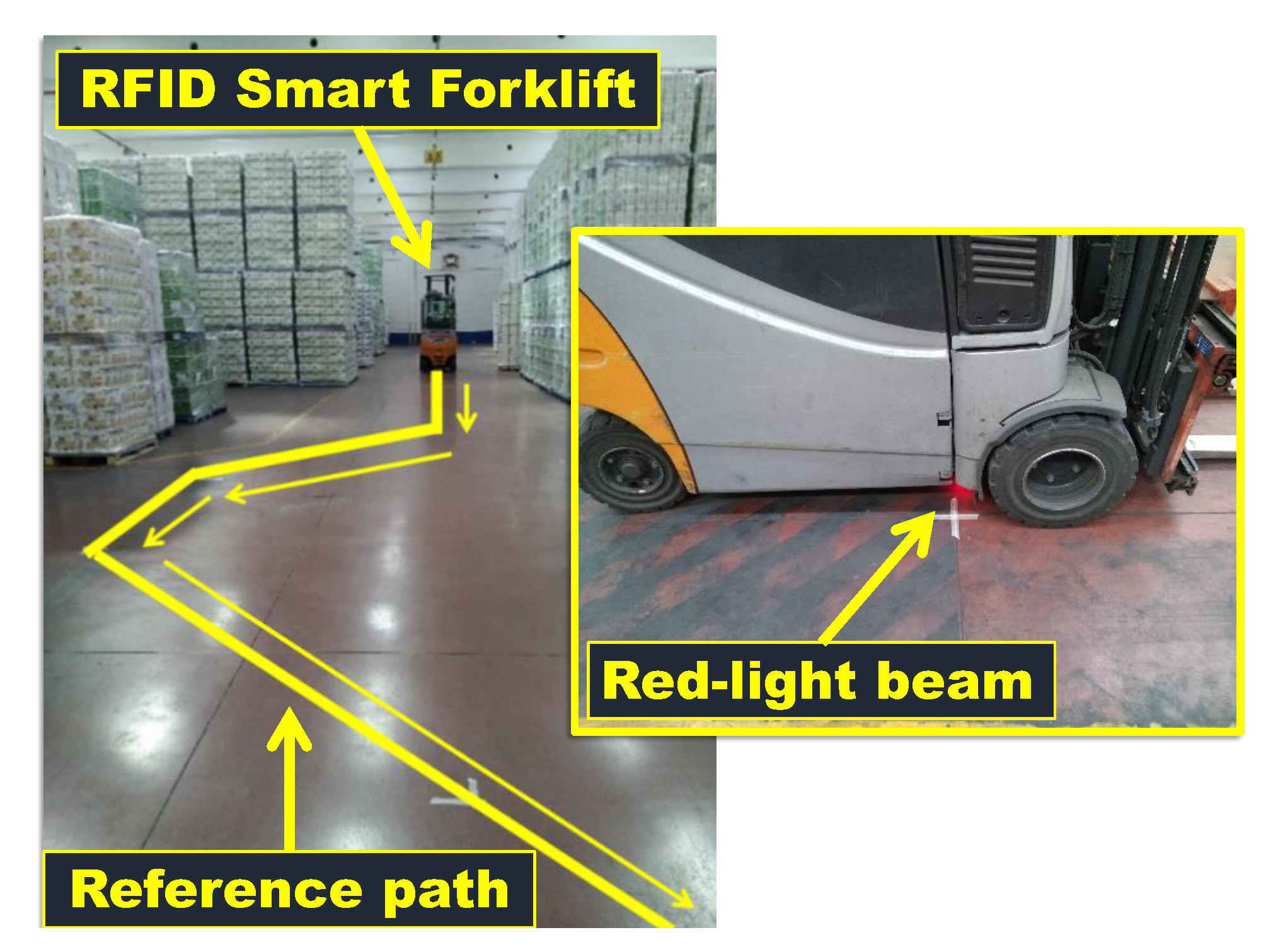
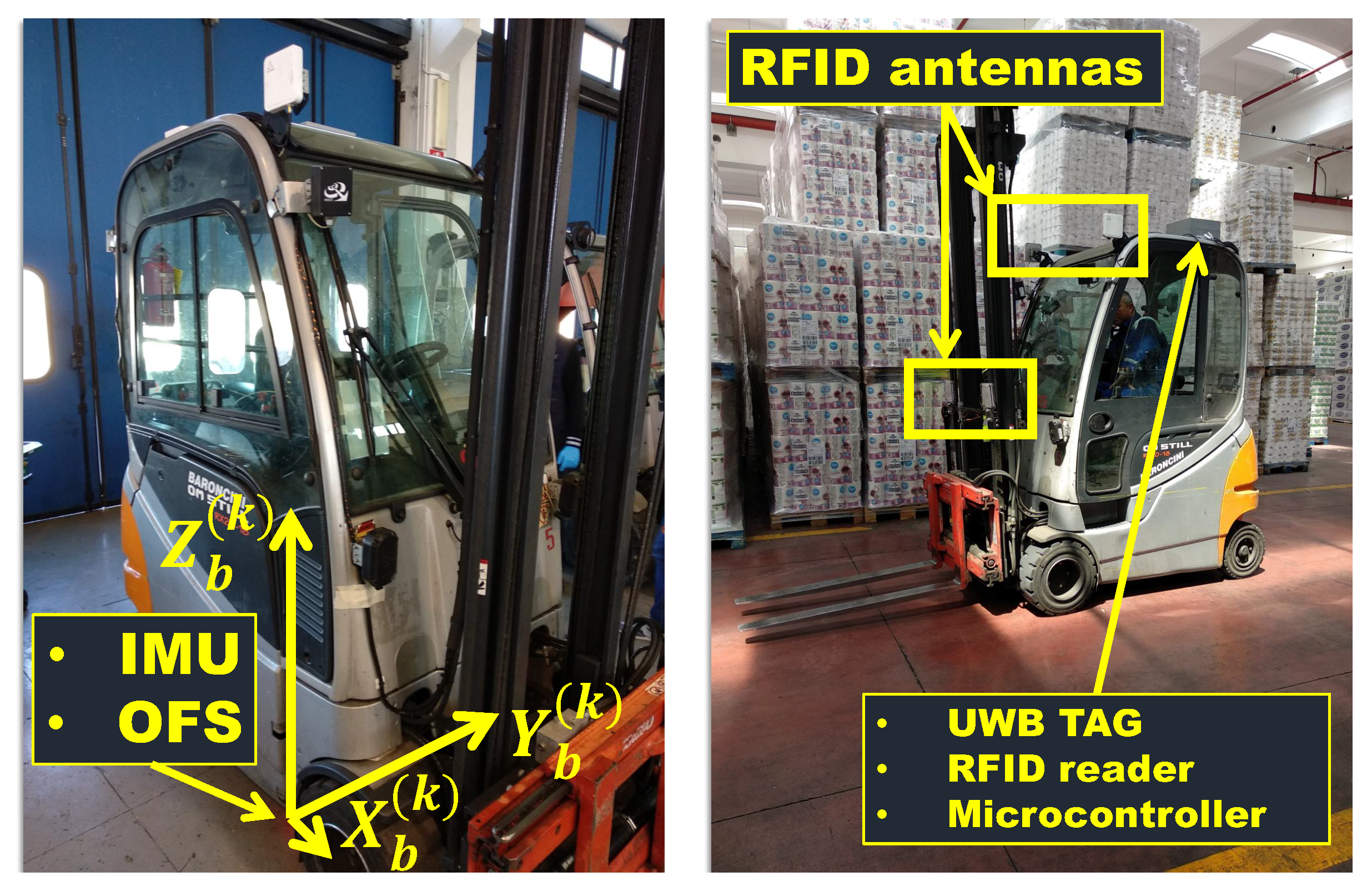
4.1. The RFID Smart Forklift
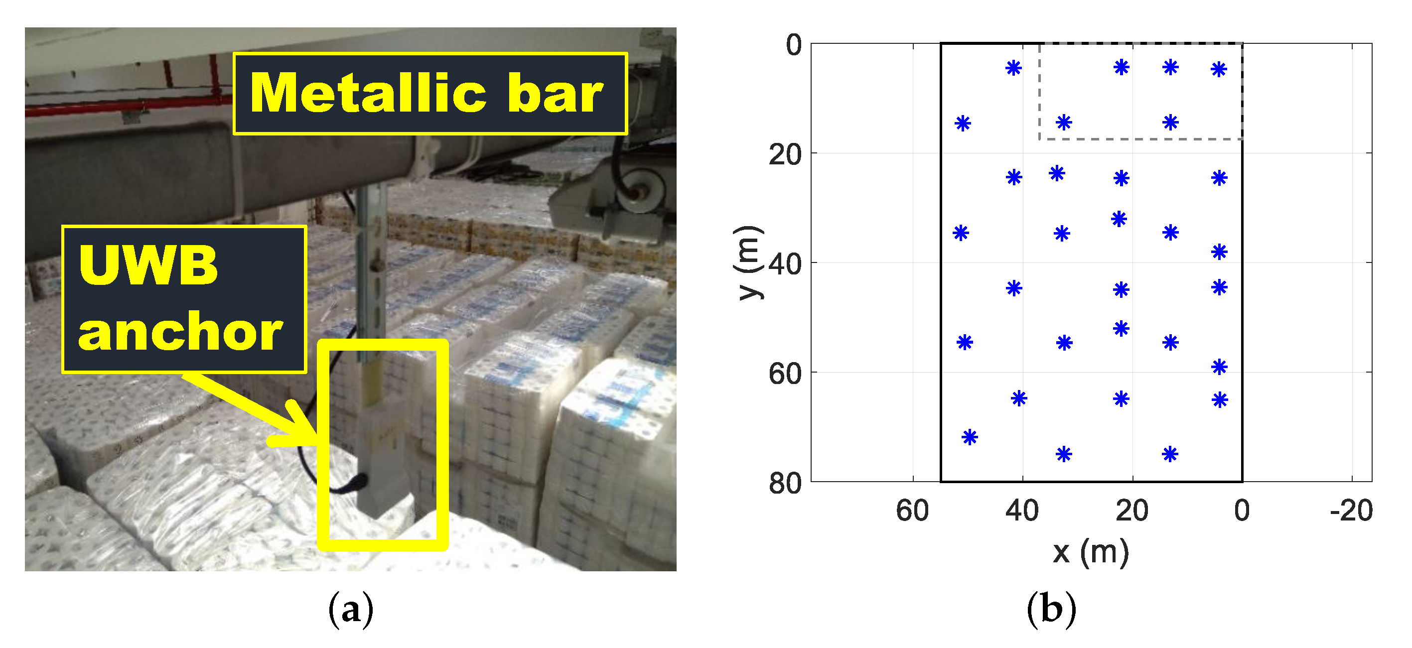
4.2. UWB Anchors
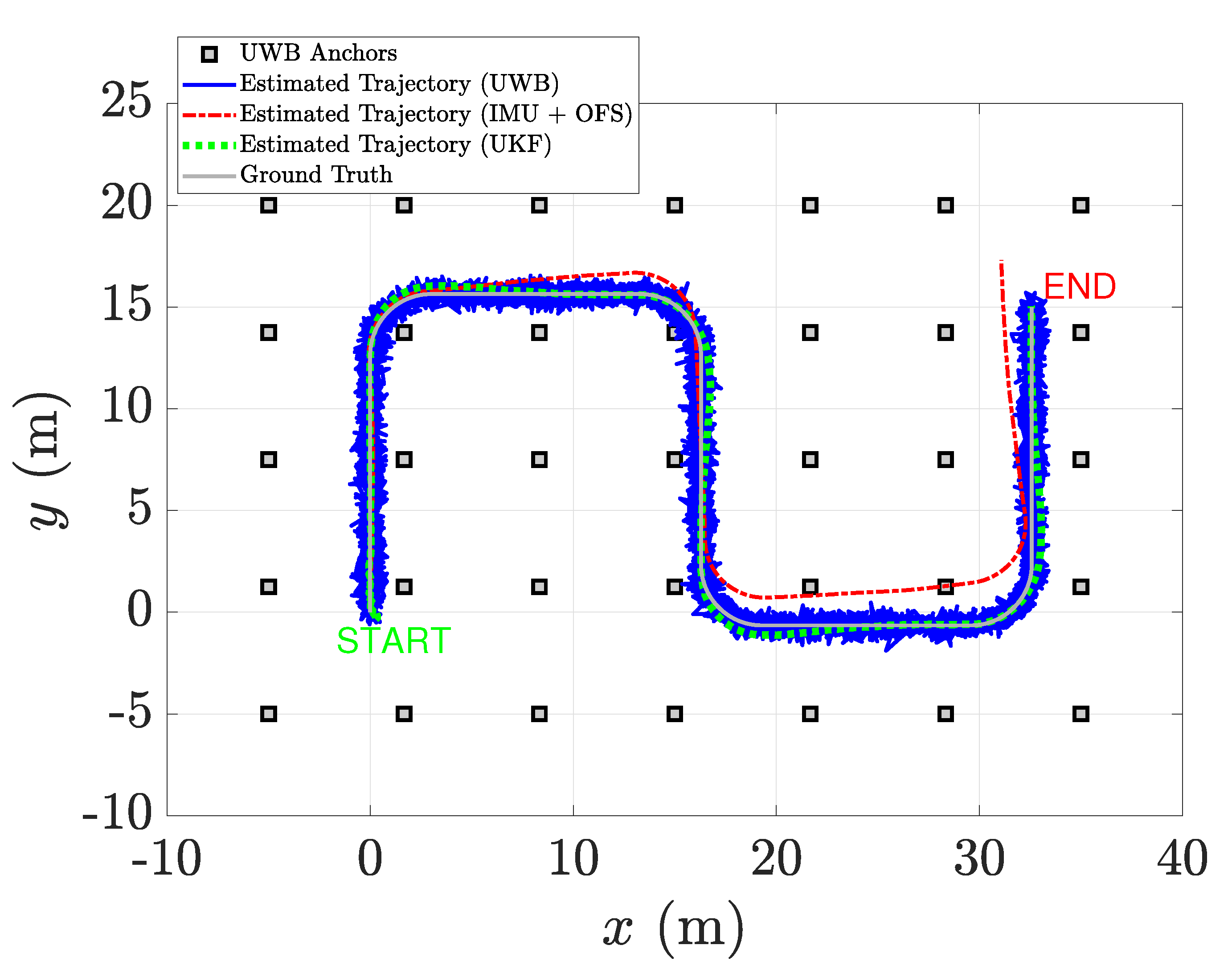
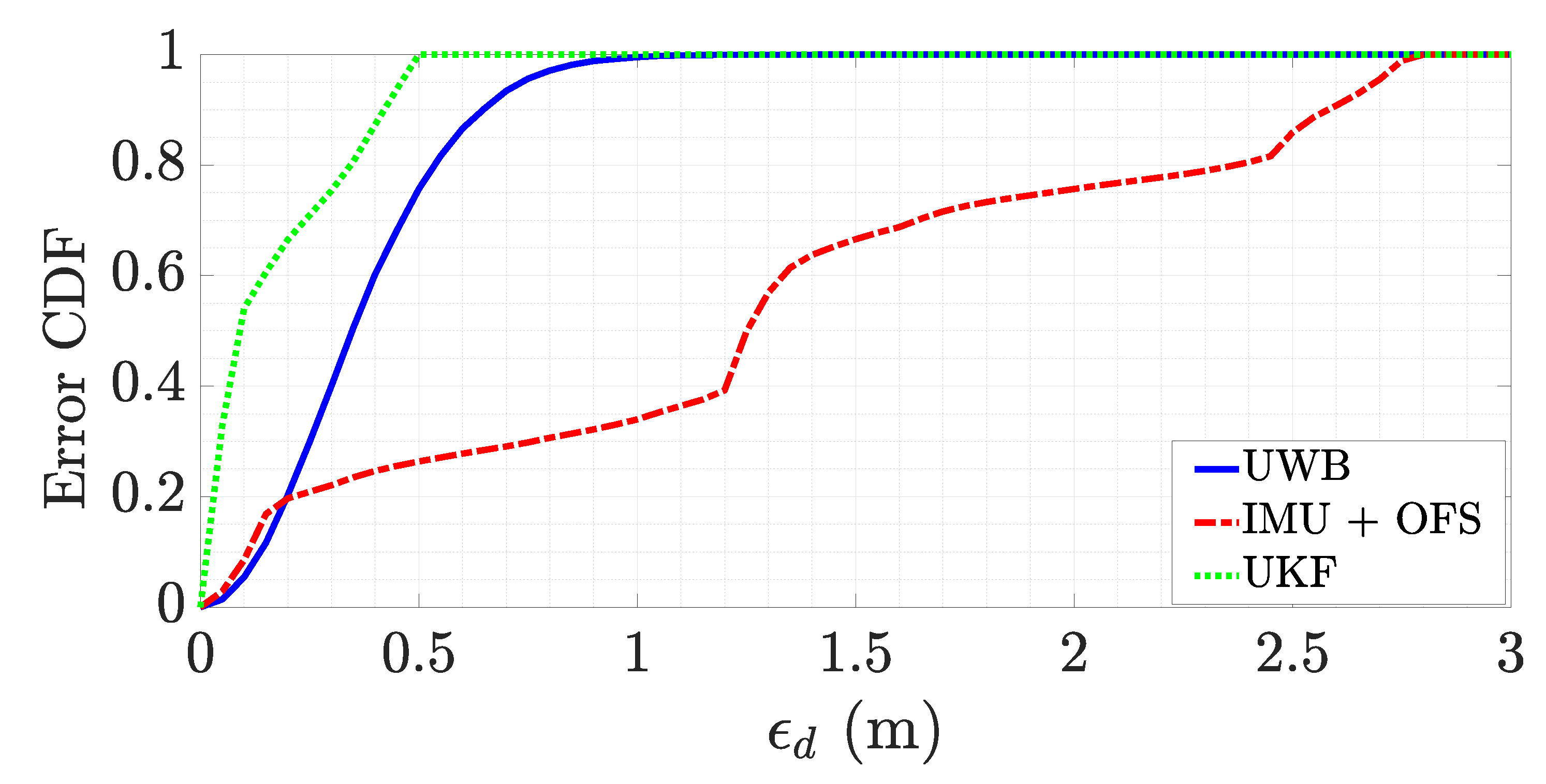
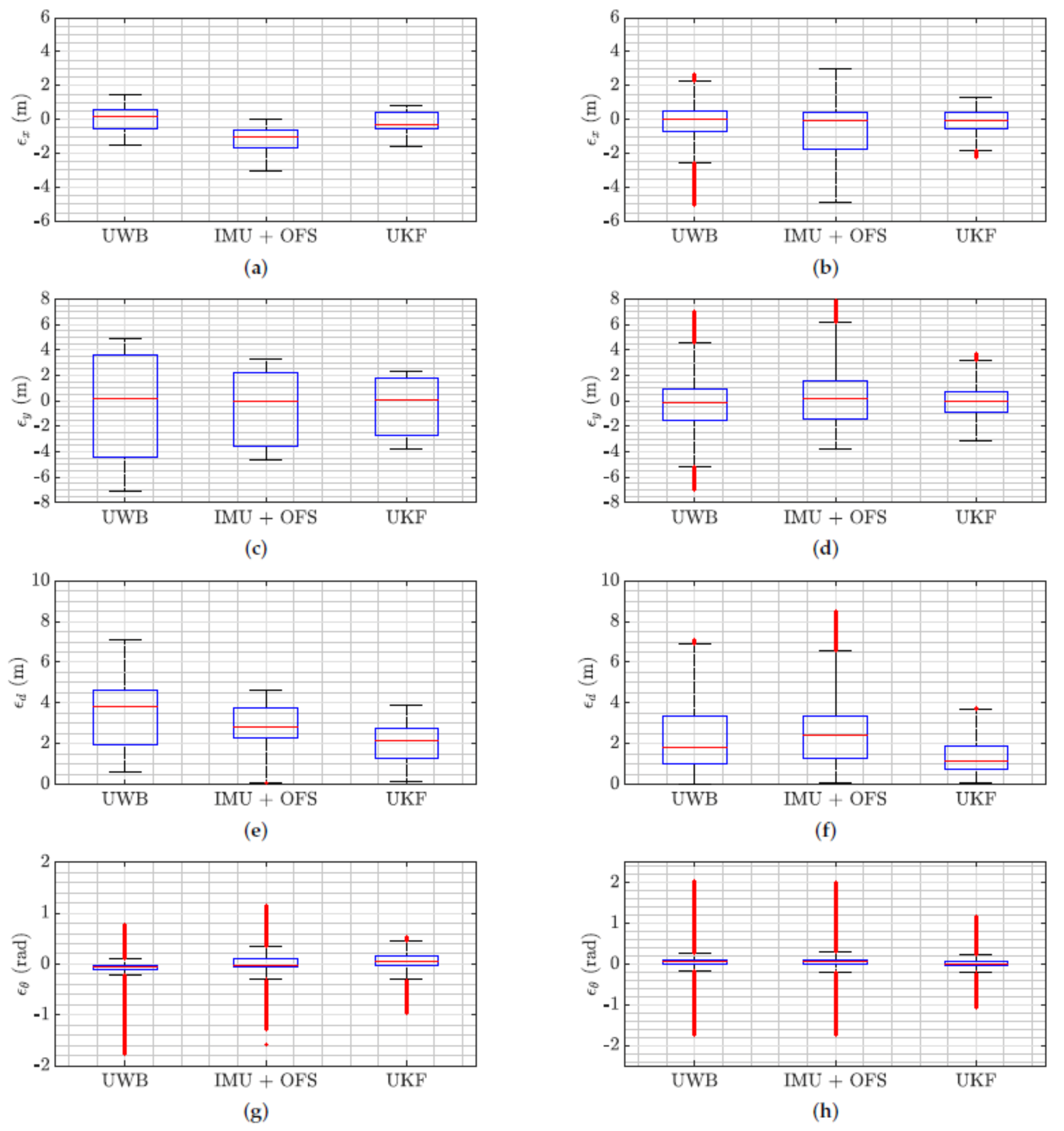
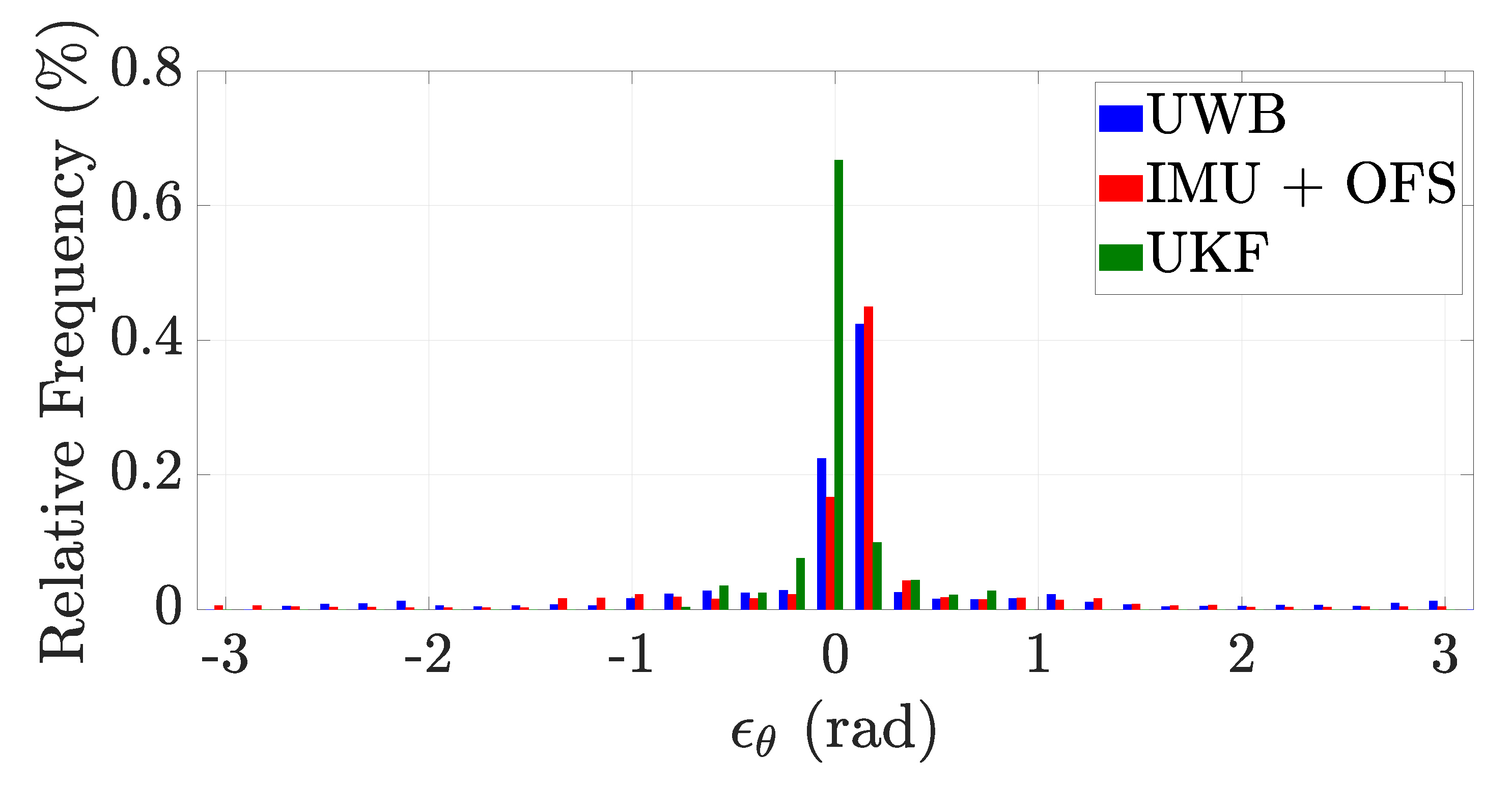
4.3. Results
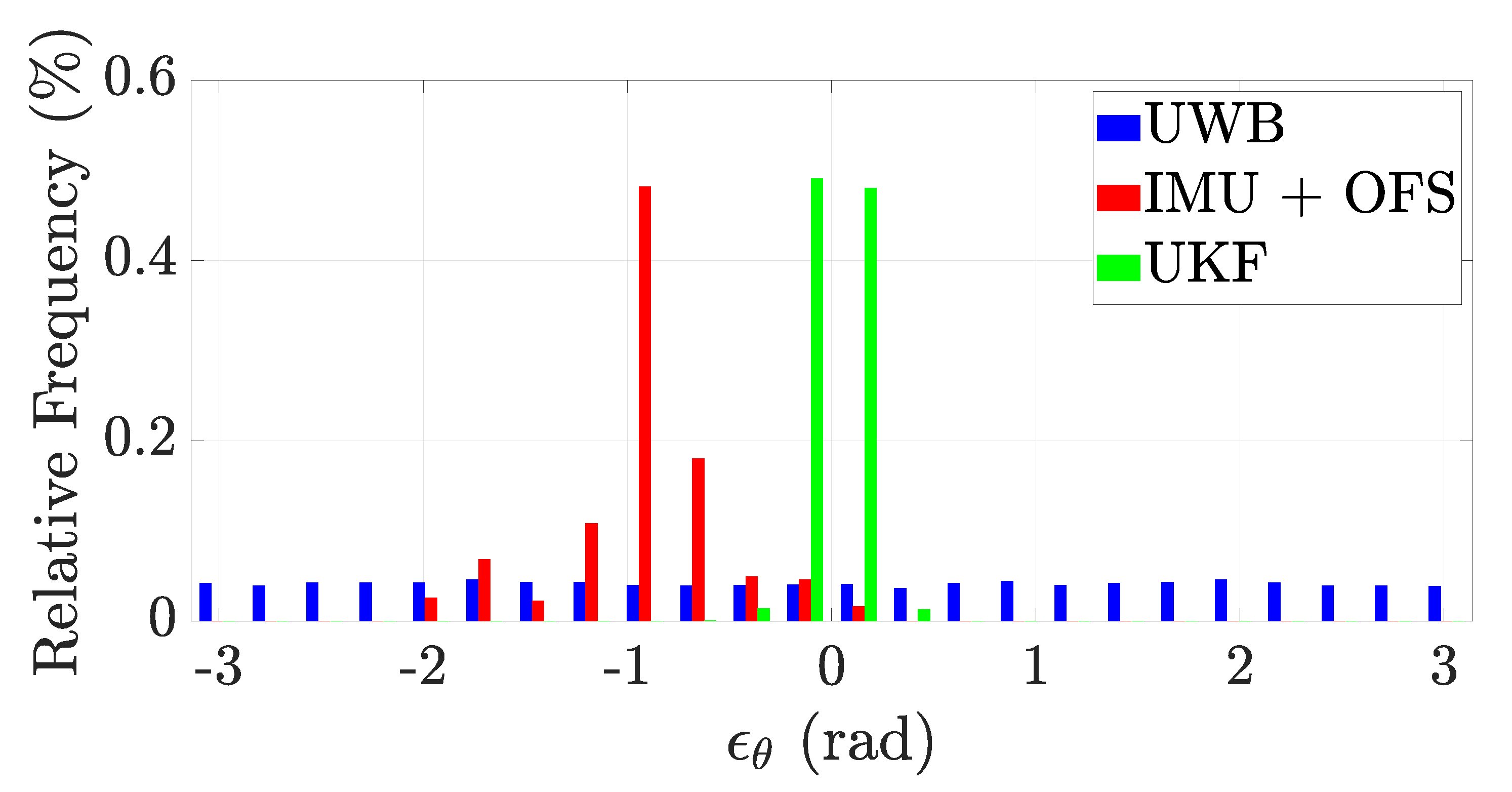
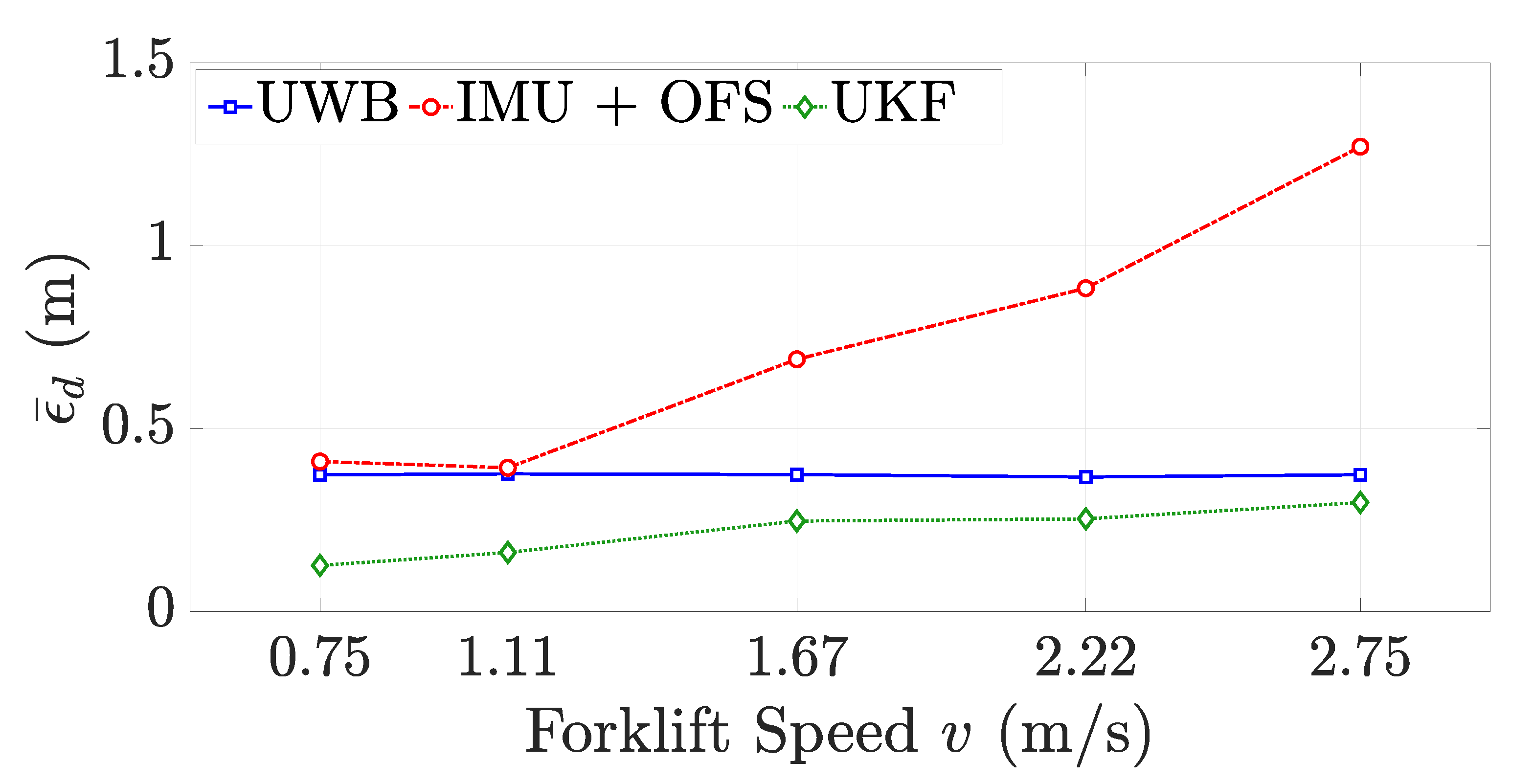
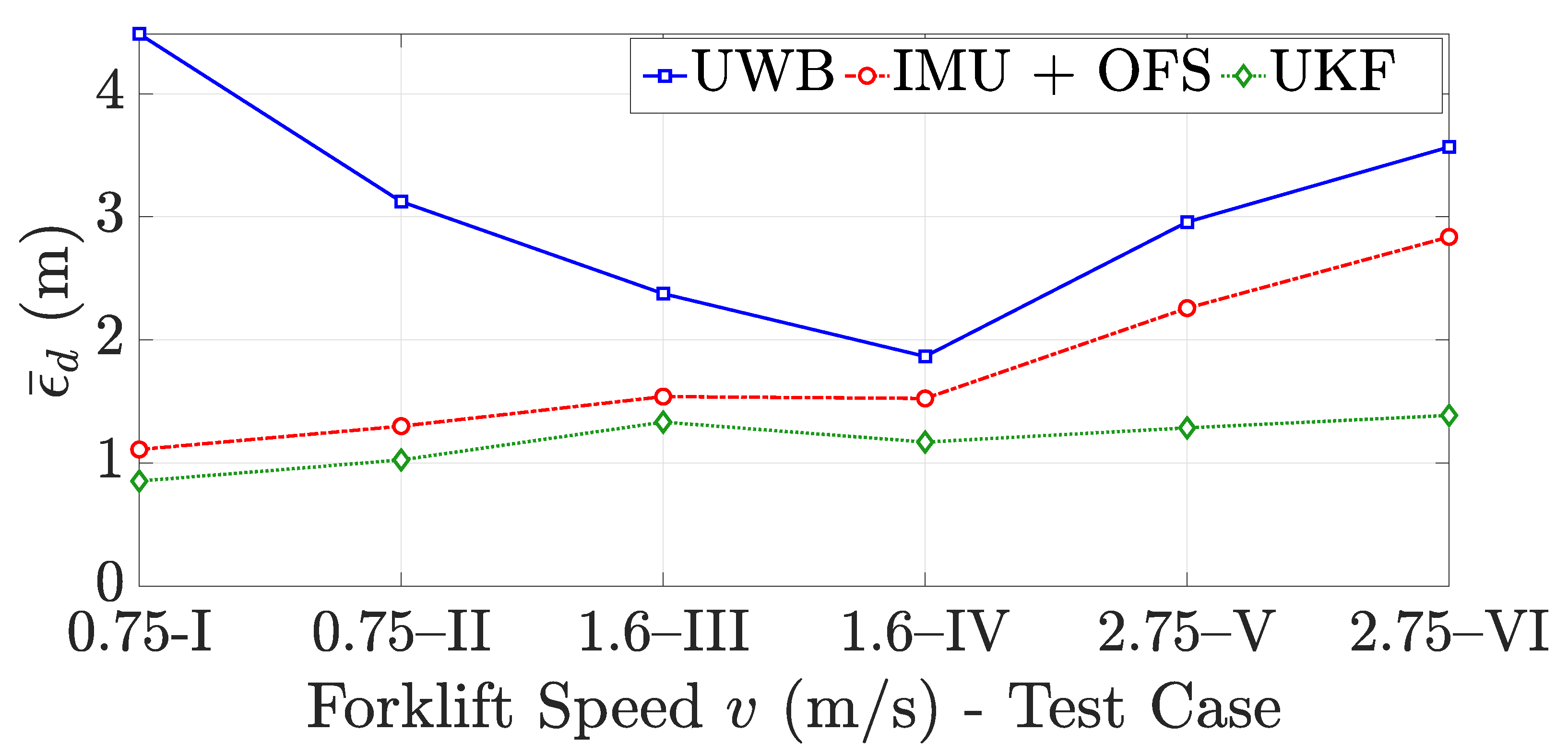
4.4. Effect of Forklift Speed
4.5. Effect of Initial Uncertainty
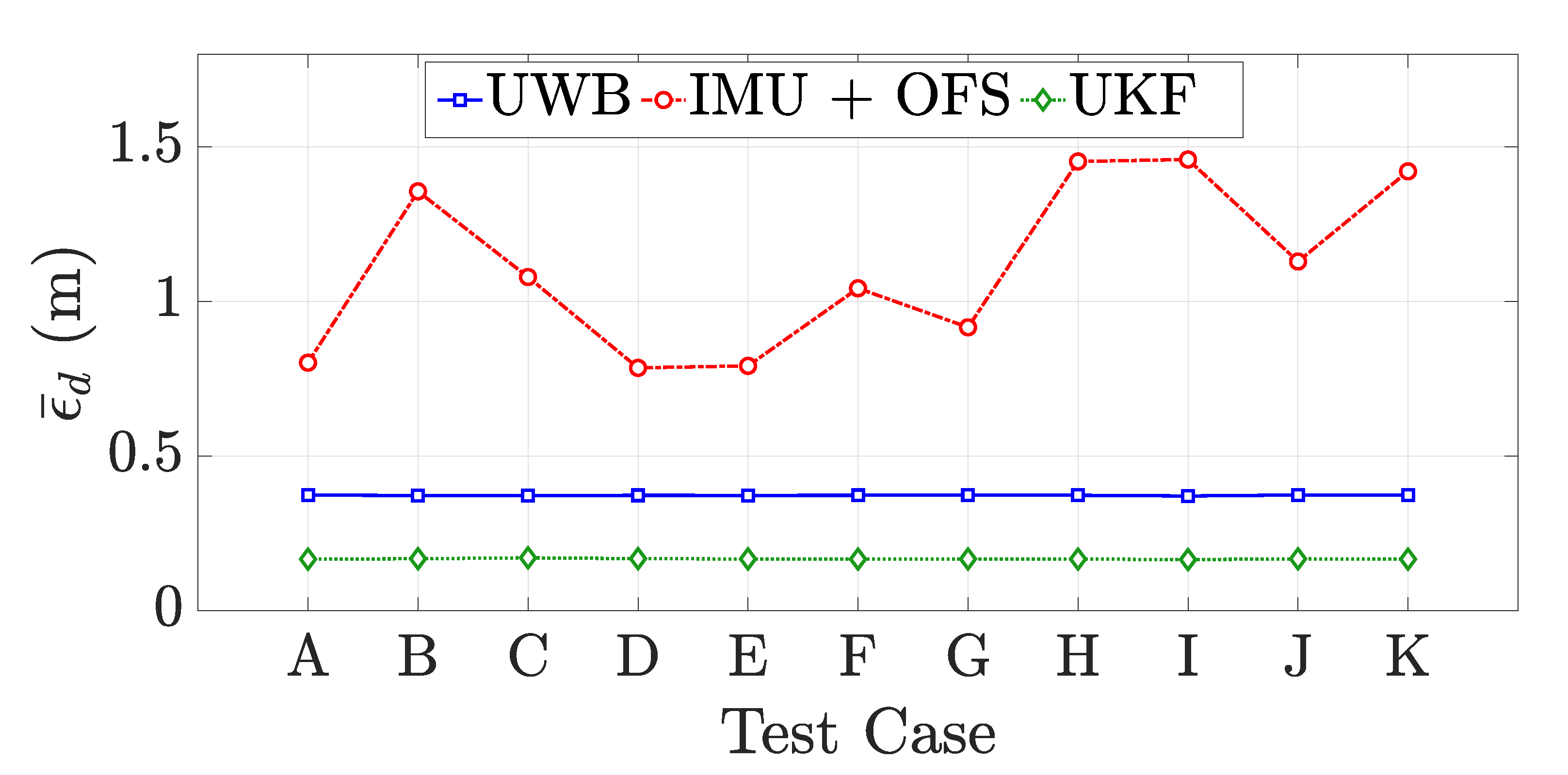
4.6. Global Performance
4.7. Computational Burden
5. Conclusions
Author Contributions
Funding
Data Availability Statement
Acknowledgments
Conflicts of Interest
References
- Laoudias, C.; Moreira, A.; Kim, S.; Lee, S.; Wirola, L.; Fischione, C. A Survey of Enabling Technologies for Network Localization, Tracking, and Navigation. IEEE Commun. Surv. Tutor. 2018, 20, 3607–3644. [Google Scholar] [CrossRef] [Green Version]
- Nepa, P.; Motroni, A.; Congi, A.; Ferro, E.M.; Pesi, M.; Giorgi, G.; Buffi, A.; Lazzarotti, M.; Bellucci, J.; Galigani, S.; et al. I-READ 4.0: Internet-of-READers for an efficient asset management in large warehouses with high stock rotation index. In Proceedings of the 2019 IEEE 5th International forum on Research and Technology for Society and Industry (RTSI), Firenze, Italy, 9–12 September 2019; pp. 67–72. [Google Scholar] [CrossRef]
- Bottani, E.; Montanari, R.; Rinaldi, M.; Vignali, G. Intelligent Algorithms for Warehouse Management. In Intelligent Techniques in Engineering Management: Theory and Applications; Kahraman, C., Çevik Onar, S., Eds.; Springer International Publishing: Cham, Switzerland, 2015; pp. 645–667. [Google Scholar] [CrossRef]
- Zhao, K.; Zhu, M.; Xiao, B.; Yang, X.; Gong, C.; Wu, J. Joint RFID and UWB Technologies in Intelligent Warehousing Management System. IEEE Internet Things J. 2020, 7, 11640–11655. [Google Scholar] [CrossRef]
- Draganjac, I.; Miklić, D.; Kovačić, Z.; Vasiljević, G.; Bogdan, S. Decentralized Control of Multi-AGV Systems in Autonomous Warehousing Applications. IEEE Trans. Autom. Sci. Eng. 2016, 13, 1433–1447. [Google Scholar] [CrossRef]
- Yassin, A.; Nasser, Y.; Awad, M.; Al-Dubai, A.; Liu, R.; Yuen, C.; Raulefs, R.; Aboutanios, E. Recent Advances in Indoor Localization: A Survey on Theoretical Approaches and Applications. IEEE Commun. Surv. Tutor. 2017, 19, 1327–1346. [Google Scholar] [CrossRef] [Green Version]
- Magnago, V.; Palopoli, L.; Buffi, A.; Tellini, B.; Motroni, A.; Nepa, P.; Macii, D.; Fontanelli, D. Ranging-Free UHF-RFID Robot Positioning Through Phase Measurements of Passive Tags. IEEE Trans. Instrum. Meas. 2020, 69, 2408–2418. [Google Scholar] [CrossRef]
- Lou, L.; Xu, X.; Cao, J.; Chen, Z.; Xu, Y. Sensor fusion-based attitude estimation using low-cost MEMS-IMU for mobile robot navigation. In Proceedings of the 2011 6th IEEE Joint International Information Technology and Artificial Intelligence Conference, Chongqing, China, 20–22 August 2011; Volume 2, pp. 465–468. [Google Scholar] [CrossRef]
- Dorigoni, D.; Fontanelli, D. An Uncertainty-driven Analysis for Delayed Mapping SLAM. In Proceedings of the 2021 IEEE International Instrumentation and Measurement Technology Conference (I2MTC), Glasgow, UK, 17–20 May 2021; pp. 1–6. [Google Scholar] [CrossRef]
- Lee, S.; Song, J.B. Robust mobile robot localization using optical flow sensors and encoders. In Proceedings of the IEEE International Conference on Robotics and Automation, ICRA ’04. 2004, New Orleans, LA, USA, 26 April–1 May 2004; Volume 1, pp. 1039–1044. [Google Scholar] [CrossRef]
- Ursel, T.; Olinski, M. Displacement Estimation Based on Optical and Inertial Sensor Fusion. Sensors 2021, 21, 1390. [Google Scholar] [CrossRef]
- Yu, J.X.; Cai, Z.X.; Duan, Z.H. Dead reckoning of mobile robot in complex terrain based on proprioceptive sensors. In Proceedings of the 2008 International Conference on Machine Learning and Cybernetics, Kunming, China, 12–15 July 2008; Volume 4, pp. 1930–1935. [Google Scholar] [CrossRef]
- Jetto, L.; Longhi, S.; Venturini, G. Development and experimental validation of an adaptive extended Kalman filter for the localization of mobile robots. IEEE Trans. Robot. Autom. 1999, 15, 219–229. [Google Scholar] [CrossRef]
- Yin, M.T.; Lian, F.L. Robot localization and mapping by matching the environmental features from proprioceptive and exteroceptive sensors. In Proceedings of the SICE Annual Conference 2010, Taipei, Taiwan, 18–21 August 2010; pp. 191–196. [Google Scholar]
- De Angelis, A.; Moschitta, A.; Carbone, P.; Calderini, M.; Neri, S.; Borgna, R.; Peppucci, M. Design and Characterization of a Portable Ultrasonic Indoor 3-D Positioning System. IEEE Trans. Instrum. Meas. 2015, 64, 2616–2625. [Google Scholar] [CrossRef]
- Comuniello, A.; De Angelis, A.; Moschitta, A. A low-cost TDoA-based ultrasonic positioning system. In Proceedings of the 2020 IEEE International Instrumentation and Measurement Technology Conference (I2MTC), Dubrovnik, Croatia, 25–28 May 2020; pp. 1–6. [Google Scholar] [CrossRef]
- Paral, P.; Chatterjee, A.; Rakshit, A. Human Position Estimation Based on Filtered Sonar Scan Matching: A Novel Localization Approach Using DENCLUE. IEEE Sens. J. 2021, 21, 8055–8064. [Google Scholar] [CrossRef]
- Scaramuzza, D.; Fraundorfer, F. Visual Odometry [Tutorial]. IEEE Robot. Autom. Mag. 2011, 18, 80–92. [Google Scholar] [CrossRef]
- Hess, W.; Kohler, D.; Rapp, H.; Andor, D. Real-time loop closure in 2D LIDAR SLAM. In Proceedings of the 2016 IEEE International Conference on Robotics and Automation (ICRA), Stockholm, Sweden, 16–21 May 2016; pp. 1271–1278. [Google Scholar] [CrossRef]
- Behrje, U.; Himstedt, M.; Maehle, E. An Autonomous Forklift with 3D Time-of-Flight Camera-Based Localization and Navigation. In Proceedings of the 2018 15th International Conference on Control, Automation, Robotics and Vision (ICARCV), Singapore, 18–21 November 2018; pp. 1739–1746. [Google Scholar] [CrossRef]
- Heo, S.; Park, C.G. Consistent EKF-Based Visual-Inertial Odometry on Matrix Lie Group. IEEE Sens. J. 2018, 18, 3780–3788. [Google Scholar] [CrossRef]
- Flueratoru, L.; Simona Lohan, E.; Nurmi, J.; Niculescu, D. HTC Vive as a Ground-Truth System for Anchor-Based Indoor Localization. In Proceedings of the 2020 12th International Congress on Ultra Modern Telecommunications and Control Systems and Workshops (ICUMT), Brno, Czech Republic, 5–7 October 2020; pp. 214–221. [Google Scholar] [CrossRef]
- Wang, F.; Lü, E.; Wang, Y.; Qiu, G.; Lu, H. Efficient Stereo Visual Simultaneous Localization and Mapping for an Autonomous Unmanned Forklift in an Unstructured Warehouse. Appl. Sci. 2020, 10, 698. [Google Scholar] [CrossRef] [Green Version]
- De Angelis, G.; Pasku, V.; De Angelis, A.; Dionigi, M.; Mongiardo, M.; Moschitta, A.; Carbone, P. An Indoor AC Magnetic Positioning System. IEEE Trans. Instrum. Meas. 2015, 64, 1267–1275. [Google Scholar] [CrossRef]
- Pasku, V.; De Angelis, A.; Dionigi, M.; Moschitta, A.; De Angelis, G.; Carbone, P. Analysis of Nonideal Effects and Performance in Magnetic Positioning Systems. IEEE Trans. Instrum. Meas. 2016, 65, 2816–2827. [Google Scholar] [CrossRef]
- Santoni, F.; De Angelis, A.; Moschitta, A.; Carbone, P. MagIK: A Hand-Tracking Magnetic Positioning System Based on a Kinematic Model of the Hand. IEEE Trans. Instrum. Meas. 2021, 70, 1–13. [Google Scholar] [CrossRef]
- Chung, H.Y.; Hou, C.C.; Chen, Y.S. Indoor Intelligent Mobile Robot Localization Using Fuzzy Compensation and Kalman Filter to Fuse the Data of Gyroscope and Magnetometer. IEEE Trans. Ind. Electron. 2015, 62, 6436–6447. [Google Scholar] [CrossRef]
- Rezazadeh, J.; Moradi, M.; Ismail, A.S.; Dutkiewicz, E. Superior Path Planning Mechanism for Mobile Beacon-Assisted Localization in Wireless Sensor Networks. IEEE Sens. J. 2014, 14, 3052–3064. [Google Scholar] [CrossRef]
- Mazuelas, S.; Bahillo, A.; Lorenzo, R.M.; Fernandez, P.; Lago, F.A.; Garcia, E.; Blas, J.; Abril, E.J. Robust Indoor Positioning Provided by Real-Time RSSI Values in Unmodified WLAN Networks. IEEE J. Sel. Top. Signal Process. 2009, 3, 821–831. [Google Scholar] [CrossRef]
- Arthaber, H.; Faseth, T.; Galler, F. Spread-Spectrum Based Ranging of Passive UHF EPC RFID Tags. IEEE Commun. Lett. 2015, 19, 1734–1737. [Google Scholar] [CrossRef]
- Koo, J.; Cha, H. Localizing WiFi Access Points Using Signal Strength. IEEE Commun. Lett. 2011, 15, 187–189. [Google Scholar] [CrossRef]
- Preusser, K.; Schmeink, A. Robust Channel Modelling of 2.4 GHz and 5 GHz Indoor Measurements: Empirical, Ray Tracing and Artificial Neural Network Models. IEEE Trans. Antennas Propag. 2021. [Google Scholar] [CrossRef]
- Biswas, J.; Veloso, M. WiFi localization and navigation for autonomous indoor mobile robots. In Proceedings of the 2010 IEEE International Conference on Robotics and Automation, Anchorage, AK, USA, 3–8 May 2010; pp. 4379–4384. [Google Scholar] [CrossRef] [Green Version]
- Motroni, A.; Buffi, A.; Nepa, P. A Survey on Indoor Vehicle Localization Through RFID Technology. IEEE Access 2021, 9, 17921–17942. [Google Scholar] [CrossRef]
- Motroni, A.; Buffi, A.; Nepa, P.; Tellini, B. Sensor Fusion and Tracking Method for Indoor Vehicles With Low-Density UHF-RFID Tags. IEEE Trans. Instrum. Meas. 2021, 70, 1–14. [Google Scholar] [CrossRef]
- Jiménez Ruiz, A.R.; Seco Granja, F. Comparing Ubisense, BeSpoon, and DecaWave UWB Location Systems: Indoor Performance Analysis. IEEE Trans. Instrum. Meas. 2017, 66, 2106–2117. [Google Scholar] [CrossRef]
- Barbieri, L.; Brambilla, M.; Trabattoni, A.; Mervic, S.; Nicoli, M. UWB Localization in a Smart Factory: Augmentation Methods and Experimental Assessment. IEEE Trans. Instrum. Meas. 2021, 70, 1–18. [Google Scholar] [CrossRef]
- De Angelis, A.; Dionigi, M.; Moschitta, A.; Giglietti, R.; Carbone, P. Characterization and Modeling of an Experimental UWB Pulse-Based Distance Measurement System. IEEE Trans. Instrum. Meas. 2009, 58, 1479–1486. [Google Scholar] [CrossRef]
- De Angelis, A.; Dionigi, M.; Moschitta, A.; Carbone, P. A Low-Cost Ultra-Wideband Indoor Ranging System. IEEE Trans. Instrum. Meas. 2009, 58, 3935–3942. [Google Scholar] [CrossRef]
- Lazzari, F.; Buffi, A.; Nepa, P.; Lazzari, S. Numerical Investigation of an UWB Localization Technique for Unmanned Aerial Vehicles in Outdoor Scenarios. IEEE Sens. J. 2017, 17, 2896–2903. [Google Scholar] [CrossRef]
- Ghanem, E.; O’Keefe, K.; Klukas, R. Testing Vehicle-to-Vehicle Relative Position and Attitude Estimation using Multiple UWB Ranging. In Proceedings of the 2020 IEEE 92nd Vehicular Technology Conference (VTC2020-Fall), Victoria, BC, Canada, 18 November–16 December 2020; pp. 1–5. [Google Scholar] [CrossRef]
- Rath, M.; Kulmer, J.; Leitinger, E.; Witrisal, K. Single-Anchor Positioning: Multipath Processing with Non-Coherent Directional Measurements. IEEE Access 2020, 8, 88115–88132. [Google Scholar] [CrossRef]
- Leitinger, E.; Meyer, F.; Hlawatsch, F.; Witrisal, K.; Tufvesson, F.; Win, M.Z. A Belief Propagation Algorithm for Multipath-Based SLAM. IEEE Trans. Wirel. Commun. 2019, 18, 5613–5629. [Google Scholar] [CrossRef] [Green Version]
- Xiao, Z.; Wen, H.; Markham, A.; Trigoni, N.; Blunsom, P.; Frolik, J. Non-Line-of-Sight Identification and Mitigation Using Received Signal Strength. IEEE Trans. Wirel. Commun. 2015, 14, 1689–1702. [Google Scholar] [CrossRef]
- Yu, K.; Wen, K.; Li, Y.; Zhang, S.; Zhang, K. A Novel NLOS Mitigation Algorithm for UWB Localization in Harsh Indoor Environments. IEEE Trans. Veh. Technol. 2019, 68, 686–699. [Google Scholar] [CrossRef]
- Wang, T.; Hu, K.; Li, Z.; Lin, K.; Wang, J.; Shen, Y. A Semi-Supervised Learning Approach for UWB Ranging Error Mitigation. IEEE Wirel. Commun. Lett. 2021, 10, 688–691. [Google Scholar] [CrossRef]
- Wymeersch, H.; Marano, S.; Gifford, W.M.; Win, M.Z. A Machine Learning Approach to Ranging Error Mitigation for UWB Localization. IEEE Trans. Commun. 2012, 60, 1719–1728. [Google Scholar] [CrossRef] [Green Version]
- Zhang, H.; Zhang, Z.; Zhao, R.; Lu, J.; Wang, Y.; Jia, P. Review on UWB-based and multi-sensor fusion positioning algorithms in indoor environment. In Proceedings of the 2021 IEEE 5th Advanced Information Technology, Electronic and Automation Control Conference (IAEAC), Chongqing, China, 12–14 March 2021; Volume 5, pp. 1594–1598. [Google Scholar] [CrossRef]
- Kolakowski, M.; Djaja-Josko, V.; Kolakowski, J. Static LiDAR Assisted UWB Anchor Nodes Localization. IEEE Sens. J. 2020. [Google Scholar] [CrossRef]
- Nguyen, T.H.; Nguyen, T.M.; Xie, L. Range-Focused Fusion of Camera-IMU-UWB for Accurate and Drift-Reduced Localization. IEEE Robot. Autom. Lett. 2021, 6, 1678–1685. [Google Scholar] [CrossRef]
- Sadruddin, H.; Mahmoud, A.; Atia, M. An Indoor Navigation System using Stereo Vision, IMU and UWB Sensor Fusion. In Proceedings of the 2019 IEEE SENSORS, Montreal, QC, Canada, 27–30 October 2019; pp. 1–4. [Google Scholar] [CrossRef]
- Xu, Y.; Shmaliy, Y.S.; Ahn, C.K.; Shen, T.; Zhuang, Y. Tightly Coupled Integration of INS and UWB Using Fixed-Lag Extended UFIR Smoothing for Quadrotor Localization. IEEE Internet Things J. 2021, 8, 1716–1727. [Google Scholar] [CrossRef]
- Zhou, H.; Yao, Z.; Lu, M. Lidar/UWB Fusion Based SLAM With Anti-Degeneration Capability. IEEE Trans. Veh. Technol. 2021, 70, 820–830. [Google Scholar] [CrossRef]
- Zhou, H.; Yao, Z.; Lu, M. UWB/Lidar Coordinate Matching Method with Anti-Degeneration Capability. IEEE Sens. J. 2021, 21, 3344–3352. [Google Scholar] [CrossRef]
- Magnago, V.; Corbalán, P.; Picco, G.P.; Palopoli, L.; Fontanelli, D. Robot Localization via Odometry-assisted Ultra-wideband Ranging with Stochastic Guarantees. In Proceedings of the 2019 IEEE/RSJ International Conference on Intelligent Robots and Systems (IROS), Macau, China, 3–8 November 2019; pp. 1607–1613. [Google Scholar] [CrossRef]
- Fontanelli, D.; Shamsfakhr, F.; Macii, D.; Palopoli, L. An Uncertainty-Driven and Observability-Based State Estimator for Nonholonomic Robots. IEEE Trans. Instrum. Meas. 2021, 70, 1–12. [Google Scholar] [CrossRef]
- Feng, D.; Wang, C.; He, C.; Zhuang, Y.; Xia, X.G. Kalman-Filter-Based Integration of IMU and UWB for High-Accuracy Indoor Positioning and Navigation. IEEE Internet Things J. 2020, 7, 3133–3146. [Google Scholar] [CrossRef]
- Arulampalam, M.; Maskell, S.; Gordon, N.; Clapp, T. A tutorial on particle filters for online nonlinear/non-Gaussian Bayesian tracking. IEEE Trans. Signal Process. 2002, 50, 174–188. [Google Scholar] [CrossRef] [Green Version]
- Julier, S.; Uhlmann, J. Unscented filtering and nonlinear estimation. Proc. IEEE 2004, 92, 401–422. [Google Scholar] [CrossRef] [Green Version]
- Wan, E.; Van Der Merwe, R. The unscented Kalman filter for nonlinear estimation. In Proceedings of the IEEE 2000 Adaptive Systems for Signal Processing, Communications, and Control Symposium (Cat. No.00EX373), Lake Louise, AB, Canada, 4 October 2000; pp. 153–158. [Google Scholar] [CrossRef]
- Decawave MDEK1001 Evaluation Kit. Available online: https://www.decawave.com/product/mdek1001-deployment-kit/ (accessed on 9 October 2021).
- Avago ADNS-3080 Optical Flow Sensor. Available online: https://datasheet.octopart.com/ADNS-3080-Avago-datasheet-10310392.pdf/ (accessed on 9 October 2021).
- STMicroelectronics VL53L0X Laser-Ranging Distance Sensors. Available online: https://www.st.com/en/imaging-and-photonics-solutions/vl53l0x.html (accessed on 9 October 2021).
- STMicroelectronics LSMDS3 Inertial Measurement Unit Platform. Available online: https://www.st.com/en/mems-and-sensors/lsm6ds3.html/ (accessed on 9 October 2021).
- RENESAS SK-S7G2 Microcontroller. Available online: https://www.renesas.com/us/en/products/microcontrollers-microprocessors/renesas-synergy-platform-mcus/yssks7g2e30-sk-s7g2-starter-kit (accessed on 9 October 2021).
- UHF-RFID Reader Impinj Speedway Revolution R420. Available online: https://support.impinj.com/hc/en-us/articles/202755388-Impinj-Speedway-RAIN-RFID-Reader-Family-Product-Brief-Datasheet (accessed on 9 October 2021).
- UHF-RFID Keonn Advantenna-p11 Antenna. Available online: https://keonn.com/components-product/advantenna-p11/ (accessed on 9 October 2021).
- UHF-RFID Alien A0501 Antenna. Available online: https://www.alientechnology.com/products/antennas/alr-a0501/ (accessed on 9 October 2021).
- Leica Flexline TS03 Manual Total Station. Available online: https://leica-geosystems.com/it-it/products/total-stations/manual-total-stations/leica-flexline-ts03 (accessed on 9 October 2021).
- Salvador, C.; Zani, F.; Biffi Gentili, G. RFID and sensor network technologies for safety managing in hazardous environments. In Proceedings of the 2011 IEEE International Conference on RFID-Technologies and Applications, Sitges, Spain, 15–16 September 2011; pp. 68–72. [Google Scholar] [CrossRef]


| Trial | [m] | [rad] |
|---|---|---|
| A | 0.1 | 0.1 |
| B | 0.2 | 0.1 |
| C | 0.4 | 0.14 |
| D | 0.6 | 0.21 |
| E | 0.8 | 0.28 |
| F | 1 | 0.35 |
| G | 1.2 | 0.42 |
| H | 1.4 | 0.49 |
| I | 1.6 | 0.56 |
| J | 1.8 | 0.63 |
| K | 2 | 0.7 |
| Test Case | Forklift Speed v [m/s] | Path-Length L [m] | Path Shape | [m] | [rad] |
|---|---|---|---|---|---|
| I | 0.75 | ∼100 | Closed-loop path | ||
| II | 0.75 | ∼100 | Closed-loop path | ||
| III | 1.6 | ∼100 | Closed-loop path | ||
| IV | 1.6 | ∼100 | Closed-loop path | ||
| V | 2.75 | ∼100 | Closed-loop path | ||
| VI | 2.75 | ∼100 | Closed-loop path | ||
| VII | 1.2 | ∼137 | Rectilinear path with U-turn | ||
| VIII | 1.2 | ∼137 | Rectilinear path with U-turn | ||
| IX | 1.28 | ∼289 | Closed-loop path |
| Test Case | (m) | (m) | (m) | (rad) | (rad) | (rad) |
|---|---|---|---|---|---|---|
| IV | 3.84 | 2.81 | 2.13 | −0.04 | −0.04 | 0.02 |
| IX | 1.77 | 2.43 | 1.17 | 0.06 | 0.06 | 0.01 |
| Test Case | Trial Duration [s] | Total Elaboration Time [s] | Number of Samples | Elaboration Time for Sample [ms] |
|---|---|---|---|---|
| I | 136 | 10.81 | 13,641 | 0.79 |
| II | 132 | 10.05 | 13,265 | 0.75 |
| III | 63 | 5.23 | 6369 | 0.82 |
| IV | 64 | 5.18 | 6432 | 0.8 |
| V | 36 | 3.43 | 3606 | 0.95 |
| VI | 36 | 3.34 | 3611 | 0.92 |
| VII | 114 | 9.28 | 11,346 | 0.81 |
| VIII | 110 | 9.05 | 11,038 | 0.82 |
| IX | 225 | 17.09 | 22,563 | 0.75 |
Publisher’s Note: MDPI stays neutral with regard to jurisdictional claims in published maps and institutional affiliations. |
© 2021 by the authors. Licensee MDPI, Basel, Switzerland. This article is an open access article distributed under the terms and conditions of the Creative Commons Attribution (CC BY) license (https://creativecommons.org/licenses/by/4.0/).
Share and Cite
Motroni, A.; Buffi, A.; Nepa, P. Forklift Tracking: Industry 4.0 Implementation in Large-Scale Warehouses through UWB Sensor Fusion. Appl. Sci. 2021, 11, 10607. https://doi.org/10.3390/app112210607
Motroni A, Buffi A, Nepa P. Forklift Tracking: Industry 4.0 Implementation in Large-Scale Warehouses through UWB Sensor Fusion. Applied Sciences. 2021; 11(22):10607. https://doi.org/10.3390/app112210607
Chicago/Turabian StyleMotroni, Andrea, Alice Buffi, and Paolo Nepa. 2021. "Forklift Tracking: Industry 4.0 Implementation in Large-Scale Warehouses through UWB Sensor Fusion" Applied Sciences 11, no. 22: 10607. https://doi.org/10.3390/app112210607
APA StyleMotroni, A., Buffi, A., & Nepa, P. (2021). Forklift Tracking: Industry 4.0 Implementation in Large-Scale Warehouses through UWB Sensor Fusion. Applied Sciences, 11(22), 10607. https://doi.org/10.3390/app112210607