Tree-Structured Regression Model Using a Projection Pursuit Approach

Abstract

In this paper, a new tree-structured regression model—the projection pursuit regression tree—is proposed. It combines the projection pursuit classification tree with the projection pursuit regression. The main advantage of the projection pursuit regression tree is exploring the independent variable space in each range of the dependent variable. Additionally, it retains the main properties of the projection pursuit classification tree. The projection pursuit regression tree provides several methods of assigning values to the final node, which enhances predictability. It shows better performance than CART in most cases and sometimes beats random forest with a single tree. This development makes it possible to find a better explainable model with reasonable predictability.

1. Introduction

Classification and regression trees are commonly applied to data, mainly for interpretability. The first regression tree was AID (automatic interaction detection [1]). At each node, AID determines the splitting rules using the sum of squared deviations as an impurity measure. It splits the data recursively and stops when the impurity measure is less than the predefined threshold value. It uses the sample mean of data in the final node as the predicted value. There are several problems with AID: overfitting, selection bias when the variables are highly correlated, and the masking problem. To overcome the overfitting problem, CART (the classification and regression tree [2]) was developed. It uses a pruning method to reduce the size of the tree to prevent overfitting. However, this increases the computational cost.

AID and CART use piecewise constant regression approaches. It is difficult to solve the masking problem with these approaches because the predictors can be used in two ways: for splitting and for fitting the model in the final node [3]. To overcome this problem, CTREE (the conditional inference tree [4]) uses a permutation test, and GUIDE (generalized, unbiased, interaction detection and estimation [5]) uses bootstrap calibration.

For decades, various algorithms have been proposed to apply complex models instead of constants values to the final nodes of the regression tree. M5 [6] and M5P [7] allow the construction of linear models at final nodes. HTL [8] allows for a nonlinear regressor at final nodes. One advantage of predicting using such complex models at final nodes over the traditional constant values is that they are generally much simpler and more accurate. Instead of making a single prediction from a complex model, ensemble models use summarize the predictions from many simple models. Tree-based ensemble models have been developed, e.g., bagging [9], boosting [10], random forests [11], BART (Bayesian Additive Regression Model [12]), and KTBoost [13]. In general, the ensemble technique is known to reduce overfitting. Accordingly, the performance of the model can be expected to be improved. Furthermore, there have been many efforts to apply tree algorithms to various regression problems like logistic regression and quantile regression [14]. Regression tree algorithms have recently extebd to the autoregressive tree model for time-series analysis [15] and the random effect tree model for panel data analysis [16]. The flexibility of fitting various types of data well is a powerful feature of regression trees. Therefore, regression tree algorithms have been developed and widely used in regression problems [17,18,19,20].

Another regression approach is projection pursuit regression (PPR [21]). This approach uses a sum of empirically determined univariate functions of the projected predictor values. To find the regression model, PPR finds the projection of the predictors, fits an empirical model with the projected predictor values and calculates the residuals. This procedure is repeated with the residuals until the residual sum of squares is very small. The final projection pursuit regression model is the sum of the empirical models in each iteration. Even though projection pursuit regression predicts the response variable quite well, it is not easy to understand the model itself, and it is quite difficult to explain patterns in the data. The projection pursuit idea is applied to improve the interpretability of the model, and a new tree with a piecewise regression approach—the projection pursuit regression tree—is proposed.

With the projection pursuit regression tree, the data analyst can explore the partitioned data as well as the data as a whole. The main difference between the general tree-based regression methods and the projection pursuit regression tree is the way they partition data. The general tree-based regression methods are focused on the space of independent variables and each final node tend to have wider-ranging values of the dependent variable. However, the projection pursuit regression tree starts from the dependent variable. This tree divides the range of the dependent variable into the number of final nodes and assigns groups in each interval. After fitting the tree, each group is assigned to one final node, and all the final nodes are ordered by values of the dependent variable. That is, the left most final node has the group with the smallest value of the dependent variable and the rightmost final node has the group with the largest value of dependent variable. Therefore, with the projection pursuit regression tree, the user can easily explore the features of the independent variables in each range of the dependent variable. To explore a more fine-grained range of the dependent variable, the user can increase the depth of the projection pursuit regression tree.

In Section 2, the general tree-based regression methods and the projection pursuit approach are reviewed. The main algorithm of the projection pursuit regression tree is in the Section 3. Our new method, the projection pursuit regression tree, is explored with wine data, and the performance of our method is compared to linear regression, CART, and the random forests in the result section. A discussion follows.

2. Regression Tree and Projection Pursuit

2.1. General Algorithm of the Regression Tree

Let Y be the dependent continuous variable and $X_1,\cdots ,X_p$ be the independent variables. For the whole procedure of the regression tree, several decisions should be made: the best independent variable $X_{k^{*}}$ among $X_1,\cdots ,X_p$ and the best cut-off $c^{*}$ in each node, the stopping rule to declare a final node, the pruning method to use to avoid overfitting, and the assignment of numerical values to the final nodes.

In each node, the regression tree uses one independent variable (for example, $X_{k^{*}}$) and separates the data in the specific node into two groups using the cut-off $c^{*}$. If $X_{k^{*}}<c^{*}$, it is assigned to the left child node. Otherwise, it is assigned to the right child node. This cutoff is determined by a predetermined rule, usually to minimize the mean squared error (MSE) for the regression tree including CART [2]. This procedure is continued until the node is declared a final node.

The stopping rule is closely connected to the model complexity. If the number of final nodes is increased, there is a high chance that it will become a complex model, and the risk of overfitting will increase. Most tree-structured methods adapt a pruning method after growing a large tree. CART uses the cost-complexity pruning method with a penalty for model complexity.

The most common values to assign to the final node are the mean of the Y values in the final node. Because of the restriction that the one value should be assigned to all observations in the same final node, the tree-structured regression methods usually have poor predictability. To improve the precision of tree-structured regression methods, several methods have suggested using linear combinations of the independent variables instead of one value [8]. In this paper, the projection pursuit method and several different models for the assignment of the final node are adapted.

2.2. Projection Pursuit

Projection pursuit is a method of finding interesting low-dimensional projections of high-dimensional data by optimizing a predetermined criterion function, called a projection pursuit index. This idea originated in [22], and the authors of [23] coined the term “projection pursuit” as a technique for exploring multivariate data. It is useful in an initial data analysis. The method can also be used to reduce multivariate data to a low-dimensional but “interesting” subspace.

The projection pursuit classification tree [24] is a classification tree that uses projection pursuit indices to separate classes. The usual tree-structured classification finds a rule to separate the data into two groups using impurity measures that determine the degree of purity in the two groups in terms of classes. A projection pursuit classification tree, on the other hand, finds a rule to separate classes into two groups. This rule uses the best projection to separate the two groups of classes with various projection pursuit indices for separating classes. One class is assigned to only one final node, and the maximum depth of the projection pursuit classification tree is at most the number of classes. Therefore, the projection pursuit classification tree constructs a simple but more understandable tree for classification. The projection coefficients of each node represent the importance of the variables in separating the classes in each node. The behaviors of the projection coefficients in each node are useful in exploring how to separate classes. This approach is extended to the regression tree.

3. Projection Pursuit Regression Tree

3.1. Construction of the Projection Pursuit Regression Tree

Multiple regression models are widely used, but it is difficult to interpret the final model, especially when there are many independent variables. Additionally, if there are nonlinear patterns between the dependent variable and independent variables, the multiple regression model is more difficult to interpret. Most regression trees have better interpretability than the ordinary multiple regression model. With recursive partitioning of the independent variable space, the regression tree discovers interesting features in each partitioned space of the independent variables. However, one of the main purposes of regression is to explain the dependent variable using the independent variables. In this paper, the dependent variable is focused and a new regression tree—the projection pursuit regression tree—is proposed.

The original idea of the projection pursuit regression tree comes from the projection pursuit classification tree [24]. In the projection pursuit regression tree, a modified approach to split nodes and assign values in the final node is used.

Let $(Y_1^{*},{\mathbf{X}}_1^{*}),\cdots ,(Y_n^{*},{\mathbf{X}}_n^{*})$ be the set of observations in a specific node and ${\mathbf{X}}_i^{*}$ be a p-dimensional vector. Then, in each node,

step 1:

Divide $Y_1^{*},\cdots ,Y_n^{*}$ into two groups: group 1 with small values and group 2 with large values (eg. Assign $Y_i^{*}$ to group 1 if $Y_i<\mathrm{median}(Y_1^{*},\cdots ,Y_n^{*})$. Otherwise, assign $Y_i^{*}$ to group 2.)

step 2:

Find the optimal 1-dimensional projection ${\alpha }^{*}$ to separate group 1 and group 2 using one of the projection pursuit indices that involves class information—the LDA, PDA, or Lr index.

step 3:

Project the data in the node onto the optimal projection ${\alpha }^{*}$, i.e.,  ${\alpha }^{*T}{\mathbf{X}}^{*}$.

If $ave\left({\alpha }^{*T}{\mathbf{X}}_i^{*}\right|Y_i^{*}\in \mathrm{group}1)\ge ave\left({\alpha }^{*T}{\mathbf{X}}_i^{*}\right|Y_i^{*}\in \mathrm{group}2)$, use ${\alpha }^{*}=-{\alpha }^{*}$ as the optimal projection.

step 4:

Find the best cut-off, c, to separate group 1 and group 2.

step 5:

Group 1 is assigned to the left node, and group 2 is assigned to the right node

In step 2, the projection pursuit index is needed to separate group 1 and group 2. The LDA index, Lr index [25], and PDA index [26] were developed to find the projection from a separating view of groups. The LDA index is based on linear discriminant analysis and is useful for finding the view that maximizes between-group variation relative to within-group variation. If the correlations among variables are high or the number of variables is relatively large compared with the number of observations, the PDA index is useful to escape the data piling problem [27] in the LDA index. The amount of penalty on correlations can be controlled with the tuning parameter $\lambda$. The PDA index with $\lambda =0$ is the same as the LDA index. Both the LDA and PDA indexes use all information in the variance-covariance matrix of the independent variables. On the other hand, the Lr index ignores the covariances among variables and uses only the variances of the independent variables ($L_{r}index\left(\mathbf{A}\right)={\left(\frac{{\sum }_{l=1}^q{\sum }_{i=1}^g{\sum }_{j=1}^{n_i}{({\overline{y}}_{i.l}-{\overline{y}}_{..l})}^r}{{\sum }_{l=1}^q{\sum }_{i=1}^g{\sum }_{j=1}^{n_i}{(y_{ijl}-{\overline{y}}_{i.l})}^r}\right)}^{1/r}$, where $y_{ijl}$ is the lth variable of the projected data in ith group jth observation and $\mathbf{A}$ is the $p\times q$ projection matrix). r determines how to calculate the distance between two points in each dimension. With different selections of indices and the parameters associated with indices, the interesting features of our data space can be found.

The projection pursuit regression tree is designed to provide an exploratory data analysis tool, and the tree structure is constructed to retain this feature. In each node, the observations are separated into a group with small Y values and a group with large Y values; the group with small Y values is assigned to the left node, and the group with large Y values is assigned to the right node. To retain this directional convention, the direction of the optimal projection in step 3 is modified.

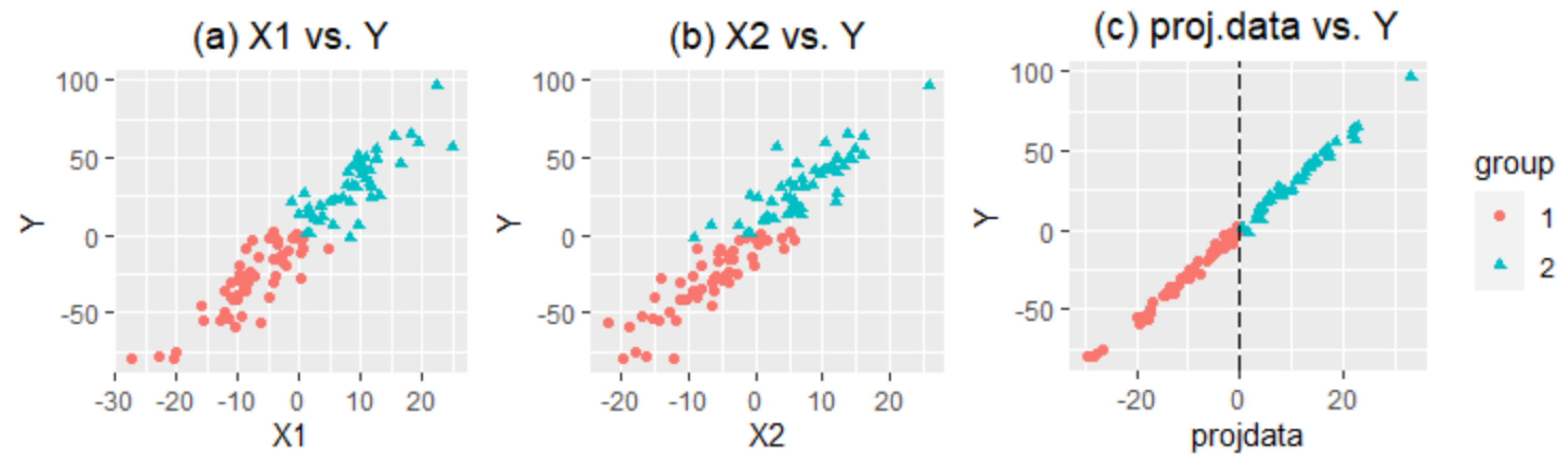
To explain how the projection pursuit regression tree works, a toy example is used. One-hundred observations with two independent variables, $X1$ and $X2$, and one dependent variable, Y, are randomly chosen. In this toy example data, $X1$ and $X2$ are highly correlated with Y (Figure 1a,b). In step 1, the data are divided into two groups: group 1 (●) and group 2 (▲). In step 2, the LDA index is used to find the optimal projection to separate group 1 and group 2. Figure 1c is the scatter plot of the projected values of $X1$ and $X2$ vs. Y.

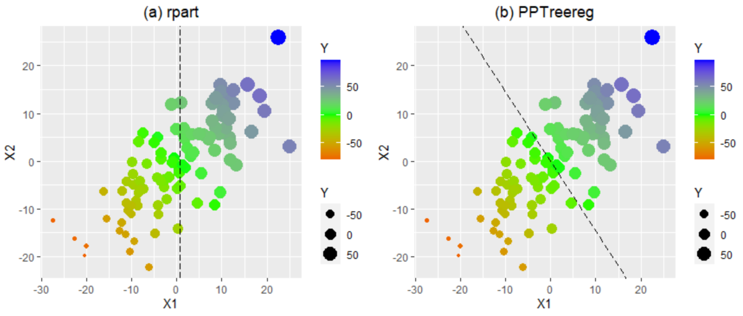
Figure 2 shows the difference between CART and the projection pursuit regression tree in dividing the space of independent variables. The dashed vertical line in the scatter plot of $X1$ and $X2$ represents the cut-off point in each method. The observations on the left/lower side of this line are assigned to the left node, and those on the right/upper side are assigned to the right node. CART uses the variable $X1$ to separate the two groups. Because CART uses one variable at a time, the separating line is parallel to the axes of the variables. In contrast, the projection pursuit regression tree uses a linear combination of the independent variables $a_{1}X1+a_{2}X2$, and this separating line can be in any direction, including the direction parallel to axes.

These procedures continue until a node is declared as a final node. To decide whether a node is final, two different ways are provided: one is for exploring data, and the other is for predicting. For the exploratory data analysis, a tree with a predefined depth can be constructed. With this approach, the projection pursuit regression tree divides the Y values into $2^{depth}$ groups and explores the properties of each group. 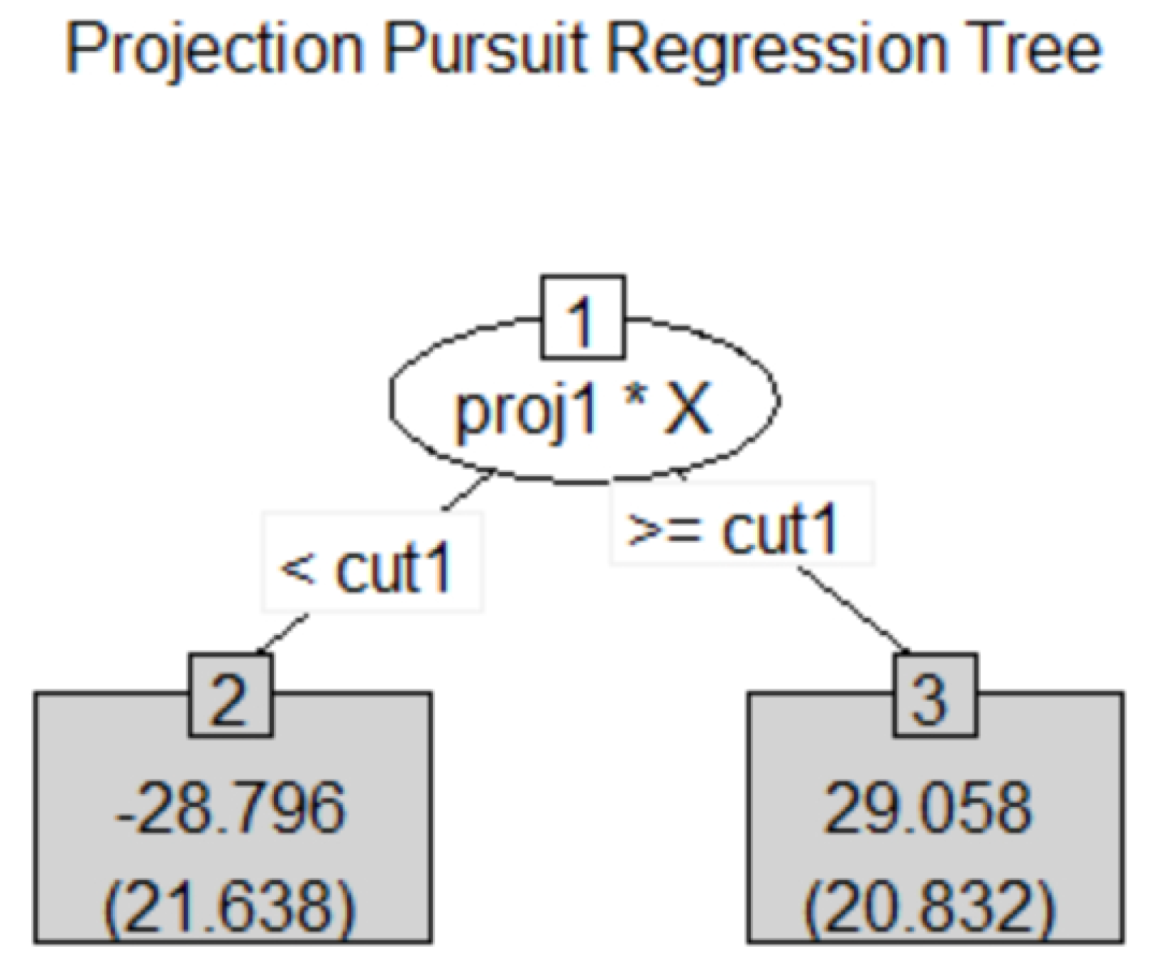Figure 3 is a simple projection pursuit regression tree for the toy example with depth 1. The data with small Y values have small $X1$ and $X2$ values, and the data with large Y values have large $X1$ and $X2$ values. For the prediction purpose, the final node is declared if the number of observations in a node is small or if the between-groups sum of squares is relatively smaller than the within-groups sum of squares. The second criterion is similar to the classical Fisher’s LDA idea.

After constructing the tree structure with the observed data, the numerical values are assigned to the final nodes. Five different models are provided in our projection pursuit regression tree to assign numerical values in the final nodes. Let $Y_{i^{*}}$ and ${\mathbf{X}}_{i^{*}}={\left[X_{i^{*}1},\cdots ,X_{i^{*}p}\right]}^T$ be the $i^{*}$th observations in a specific final node, $i^{*}=1,\cdots ,n^{*}$, where $n^{*}$ is the number of observations in the node and ${\alpha }^{*}$ is the best projection of the previous node. Then, for a new observation ${\mathbf{X}}^{*}={\left[X_1^{*},\cdots ,X_p^{*}\right]}^T$,

Model 1:

${\widehat{Y}}^{*}=\frac{1}{n^{*}}{\sum }_{i^{*}=1}^{n^{*}}{Y}_{i^{*}}$

Model 2:

${\widehat{Y}}^{*}$ = median($Y_1,\cdots ,Y_{n^{*}}$)

Model 3:

${\widehat{Y}}^{*}={\widehat{\beta }}_0+{\widehat{\beta }}_1·proj{X}^{*}$

where ${\widehat{\beta }}_0$ and ${\widehat{\beta }}_1$ are estimated from the simple linear regression model with new variable $proj{X}^{*}={{\alpha }^{*}}^T{\mathbf{X}}^{*}$ that is generated from the optimal projection ${\alpha }^{*}$.

Model 4:

${\widehat{Y}}^{*}={\widehat{\beta }}_0+{\widehat{\beta }}_1{X}_1^{*}+\cdots +{\widehat{\beta }}_p{X}_p^{*}$

where ${\widehat{\beta }}_0,\cdots ,{\widehat{\beta }}_p$ are estimated from the multiple linear regression model with all independent variables.

Model 5:

${\widehat{Y}}^{*}={\widehat{\beta }}_0+{\widehat{\beta }}_1{X}_{1^{*}}^{*}+\cdots +{\widehat{\beta }}_{p^{*}}{X}_{p^{*}}^{*}$

where ${\widehat{\beta }}_0,\cdots ,{\widehat{\beta }}_{p^{*}}$ are estimated from the multiple linear regression model with the selected $p^{*}$ independent variables.

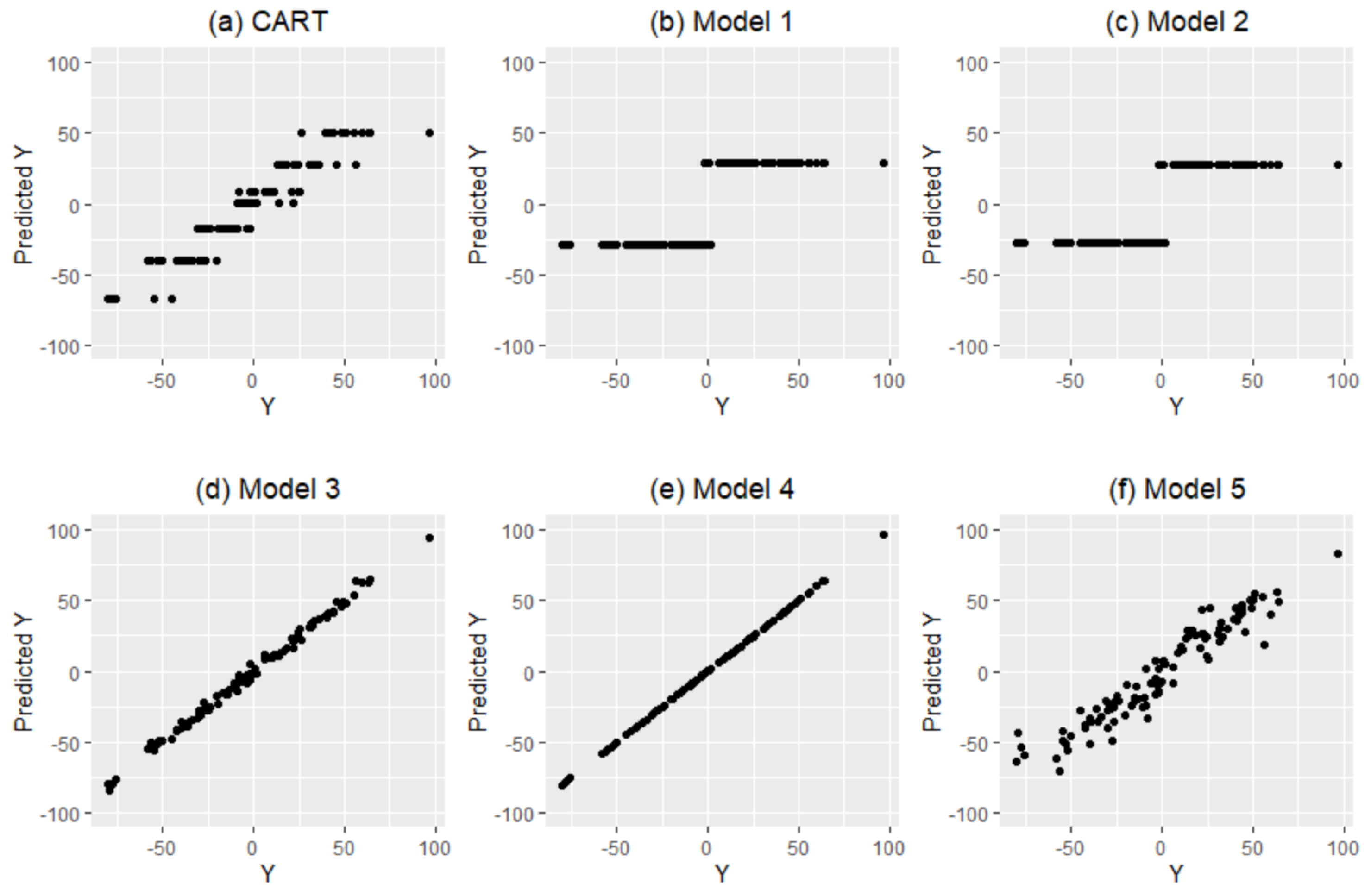
In Model 5, $p^{*}$ is the predetermined number and the independent variables are selected using the correlations with Y. Figure 4 shows how CART and the projection pursuit regression tree with Models 1–5 assign values to the final node. For Figure 4, the toy example data is fitted to a projection pursuit regression tree with depth 1 (Figure 3). The result of CART has 7 final nodes, and each node is assigned to one value. In Models 1 and 2, the mean and median of the small Y group are assigned to the left node and the mean and median of the large Y group are assigned to the right node. For Model 3, ${\widehat{Y}}^{*}={\widehat{\beta }}_0+{\widehat{\beta }}_1·proj{X}^{*}$ is used to predict the Y values, where $proj{X}^{*}$ is the projected data of the first node. The ${\widehat{Y}}^{*}={\widehat{\beta }}_0+{\widehat{\beta }}_{1}X1+{\widehat{\beta }}_{2}X2$ model is used for Model 4, and ${\widehat{Y}}^{*}={\widehat{\beta }}_0+{\widehat{\beta }}_{1}X1$ is used for Model 5 ($p^{*}=1$).

The MSEs of the fitted values with multiple linear regression, CART, the random forest for regression [11], and the projection pursuit regression tree with various models for the final node are summarized in

Table 1. MSEs of the toy example with lm, randomForest, rpart, and the projection pursuit regression tree.

				Projection Pursuit Regression Tree
Method	Lm	RandomForest	Rpart	Model 1	Model 2	Model 3	Model 4	Model 5
MSE	0.0027	29.83	124.83	444.02	447.16	6.47	0.0025	121.67

. For the comparison, the lm, randomForest, and rpart functions in R are used. In this toy example, lm and the projection pursuit regression tree with Model 4 show the best performance. randomForest shows poor performance on these data. The MSE of randomForest is much higher than that of the lm method. The result of rpart is worse than that of randomForest. In the projection pursuit regression tree, the performances of various models are quite different. The MSEs of the Model 1 and 2 are much higher than that of rpart. This result is mainly due to the simple tree with depth 1 (the depth of the rpart model is 3). If a more complex tree with a greater depth is used, the performance of Models 1 and 2 can be improved. Model 5 shows similar performance to rpart, and Model 3 shows better performance than randomForest. The performance of Model 4 is similar to that of lm. From this result, it is confirmed that the predictability with various models of assigning final values can be improved.

3.2. Features of the Projection Pursuit Regression Tree

The projection pursuit regression tree is developed to explore data in each partitioned data space instead of the whole data space by focusing on the value of the dependent variable (Y). This tree always divides the data by Y values; the observations with smaller Y values are assigned to the left node and the observations with larger Y values are assigned to the right node. After fitting the projection pursuit regression tree, all final nodes are sorted by their estimated values—the node that is furthest to the left has the smallest estimated value, and the rightmost node has the largest estimated value. Therefore, with this tree structure, the most important variables for large or small Y values can be determined.

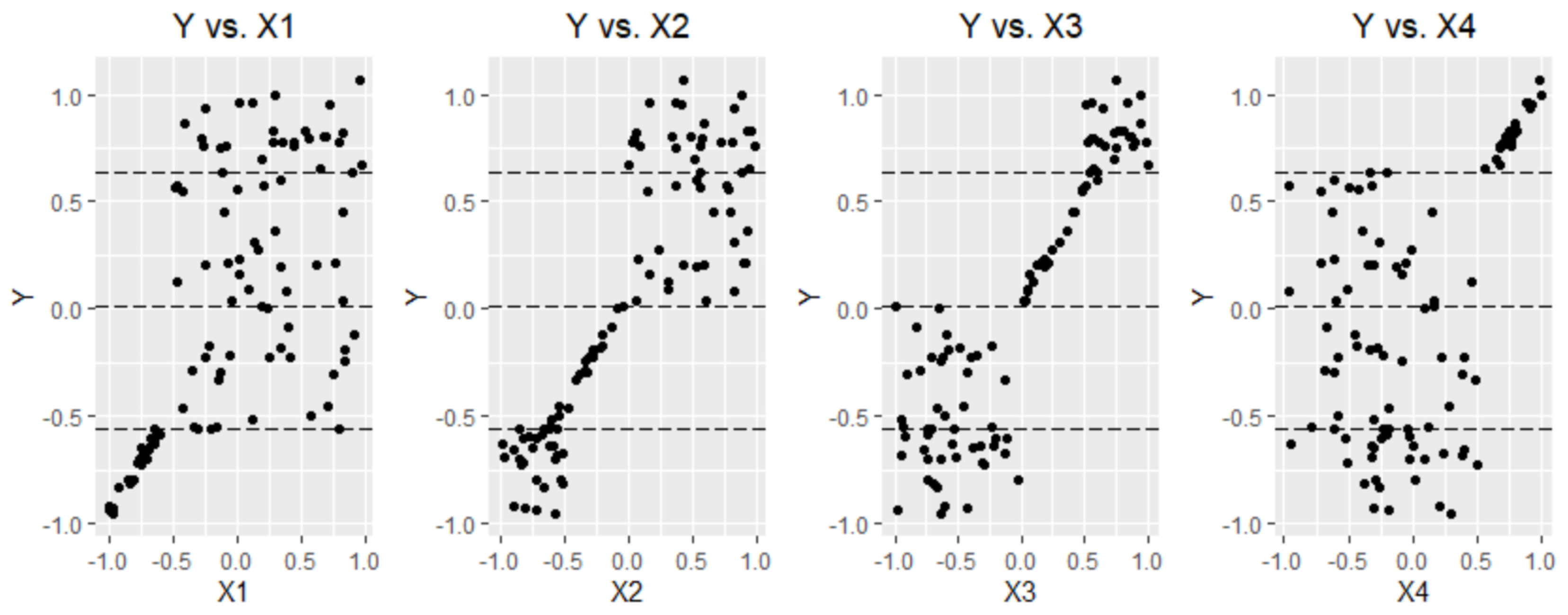
To examine this feature of the projection pursuit regression tree more deeply, 100 bservations with one dependent variable and four independent variables are simulated. Let Q1, Q2, and Q3 be the 25%, 50%, and 75% quartiles of Y. The Y values are divided into four groups—G1, G2, G3 and G4—with these quartiles. $X1$ is linearly associated with Y in G1 and does not have any relation with Y in the other groups. Similarly, $X2$ shows a linear relationship with Y only in G2, X3 shows an association with Y only in G3, and X4 shows an association with Y only in G4. The structures of the data are presented in Figure 5. The relationships between Y and the Xs depend on the range of Y values.

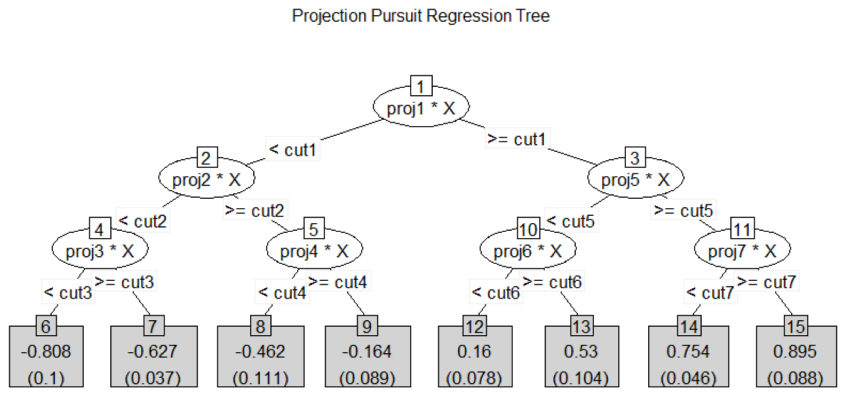
Figure 6 shows the result of the projection pursuit regression tree with depth 3, and 

Table 2. The projection coefficients of each node in the projection pursuit regression tree and the importance measure of randomForest.

Projection Pursuit Regression Tree
Coefficients	X1	X2	X3	X4
node 1	0.017	2.534	3.073	−0.368
node 2	2.231	3.257	−0.360	−0.530
node 3	−0.023	−0.464	3.031	2.569
node 4	3.981	0.386	−0.073	0.002
node 5	0.275	3.971	0.378	−0.100
node 10	−0.074	0.325	3.985	−0.080
node 11	0.209	0.233	0.468	3.960
overall importance	75.946	187.443	199.800	98.442
randomForest
	X1	X2	X3	X4
importance measure	6.724	11.360	11.678	7.151

shows the coefficients of projection in each node and the overall importance measure of the projection pursuit regression tree as well as the importance measure of the random forest for regression. The length of the projection is stick to one and the value of the projection coefficient depends on the number of variables. For consistent decision, the number of variables in each coefficient is multiplied for comparison. The projection coefficients of projection pursuit in each node show the role of each variable in separating the left and the right nodes. If the absolute value of a coefficient is large (great than 1), the corresponding variable plays an important role in this separation.

In node 1, all Y values are divided into two groups—(G1, G2) and (G3, G4). To separate the smaller Y groups (G1, G2) from the larger Y groups (G3, G4), $X2$ and X3 should play an important role, as indicated by the coefficients of node 1. Additionally, $X1$ and $X2$ are important for separating G1 and G2. This separation occurs in node 2 and the coefficients of node 2 are large in $X1$ and $X2$. In separating G3 and G4 in node 3, $X3$ and $X4$ are important. To separate G1 into smaller and larger groups (node 4), $X1$ should primarily be used. Additionally, $X2$ should be used for G2 (node 5), $X3$ should be used for G3 (node 10), and $X4$ should be used for G4 (node 11). All these features can be found in Table 2 by the corresponding coefficients of each node in the projection pursuit regression tree. Table 2 show the importance measure of the random forest for regression. The order of importance is $X3$, $X2$, $X1$, and $X4$. It shows the same result of the overall importance of the projection pursuit regression tree.

Table 3. MSEs of lm, randomForest, rpart, and the projection pursuit regression tree.

				Projection Pursuit Regression Tree
Method	Lm	RandomForest	Rpart	Model 1	Model 2	Model 3	Model 4	Model 5
MSE	0.0353	0.0096	0.0083	0.0067	0.0073	0.0024	0.0024	0.0017

shows MSE of multiple regression line (lm), randomForest, rpart and 5 models of the projection pursuit regression tree. According to Table 3, all methods in the projection regression tree show better performance than the other three methods, lm, randomForest, and rpart.

4. Results

4.1. Application: White and Red Wine Data

To explain how to explore data and find interesting features with the projection pursuit regression tree, wine data from the UCI Machine Learning repository (“https://archive.ics.uci.edu/ml/datasets.php” [28]; accessed on 15 September 2021) is used. These data are for Portugal wines. Eleven sensory variables were collected from 4898 white wines and 1599 red wines. Additionally, the quality of wines was evaluated. The wine quality is between 0 (very bad) and 10 (excellent). In this paper, the projection pursuit regression tree is fitted to the white wine data and red wine data separately and compare the differences between white wine and red wine.

For this exploration, the projection pursuit regression tree is fitted first. Figure 7 shows the final projection pursuit regression tree.

Table 4. Projection pursuit coefficients in each node for the white and red wine.

Variable Name	White Wine				Red Wine
	Node 1	Node 2	Node 3	Node 4	Node 1	Node 2	Node 3	Node 4
fixed acidity	1.56	−0.24	1.78	−0.04	4.34	1.04	−4.32	−5.05
volatile acidity	−1.24	−4.71	0.31	−2.71	−2.34	−4.49	3.71	−4.84
citric acid	−0.17	0.14	0.51	0.33	1.24	−1.83	1.92	−1.36
residual sugar	6.30	5.08	7.20	5.62	2.61	−0.02	−1.00	−2.91
chlorides	−0.23	0.12	2.78	0.14	−2.26	−1.47	−3.76	−0.96
free sulfur dioxide	0.98	1.48	2.69	−0.037	−0.42	2.28	0.50	0.52
total sulfur dioxide	−0.41	−0.74	−1.07	1.63	−1.61	−4.79	−2.02	2.36
density	−7.80	−4.18	−6.62	−7.70	−5.08	0.04	0.43	5.51
pH	2.03	0.96	2.24	0.25	0.20	−0.61	−6.10	−4.69
sulphates	1.26	1.48	−0.68	0.35	4.37	3.70	2.83	−0.76
alcohol	3.10	7.04	0.45	−4.45	5.96	7.22	4.45	1.41

shows the best projection coefficients for all internal nodes. Node 1 divides the data into a high-quality group (quality $\ge 7$) and a low-quality group (quality $\le 6$). In both wines, if the alcohol is high and the density is low, the wine is classified in the high-quality group. Additionally, there are differences in the significant sensory variables between the white and red wine quality. White wines with high residual sugar are classified in the high-quality group. In contrast, red wines with high fixed acidity and high sulphates are classified in the high-quality wine group.

In node 2, the projection pursuit regression tree divides the low-quality group into two small groups, one with quality 6 and the other with the lowest quality (≤5). In white wine, high volatile acidity, low residual sugar, high density, and low alcohol tend to produce lower quality, and red wines with high volatile acidity, high total sulfur dioxide, low sulphates, and low alcohol have the lowest quality. Node 3 divides the top-quality group (≥8) and the group with quality 7. High residual sugar and low density are still important to classify a wine as a top-quality white wine. The red wine shows a bit of complicated sensory evaluation. Low fixed acidity, high volatile acidity, low chlorides, low pH, and high alcohol tend to produce top-quality wine.

Node 4 divides the lowest-quality group (≤4) and the group with quality 5. White wines with low residual sugar, high density, and high alcohol have the lowest quality. In red wine, high acidity, low density, and high pH tend to produce the lowest quality.

Table 5. Importance measures of the white wine data.

Projection Pursuit Regression Tree		RandomForest
Variables	Importance	Variables	Importance
density	646.23	alcohol	621.77
residual sugar	587.62	density	413.10
alcohol	436.91	volatile acidity	389.11
volatile acidity	252.90	free sulfur dioxide	385.95
pH	143.63	chlorides	306.12
free sulfur dioxide	117.04	total sulfur dioxide	293.33
sulphates	114.89	residual sugar	277.97
fixed acidity	91.90	pH	258.04
total sulfur dioxide	75.78	citric acid	255.65
chlorides	41.67	fixed acidity	235.73
citric acid	21.52	sulphates	222.10

shows the importance measures of each variable in the white wine data. For the projection pursuit regression tree, the importance measure of each variable is a weighted sum of the absolute value of the projection coefficients of each node. For the weights, the number of observations in each node is used. In the white wine data, four variables—density, residual sugar, alcohol, and volatile acidity—have important roles in dividing five groups; the lowest-quality group, the groups of quality 5, 6, and 7, and the top-quality group. These results are compared with the importance measure in randomForest. Alcohol, density, volatile acidity, and free sulfur dioxide are the four most important variables in randomForest. The roles of residual sugar and free sulfur dioxide are quite different in the two methods. Residual sugar is a very important variable in the projection pursuit regression tree but not in randomForest, and free sulfur dioxide is important in randomForest but not in the projection pursuit regression tree.

Table 6. Importance measures of the red wine data.

Projection Pursuit Regression Tree			RandomForest
ID	Variables	Importance	ID	Variables	Importance
X11	alcohol	545.82	X11	alcohol	194.85
X2	volatile acidity	364.27	X10	sulphates	135.30
X10	sulphates	336.86	X2	volatile acidity	127.13
X8	fixed acidity	331.98	X8	density	86.55
X1	density	313.67	X7	total sulfur dioxide	79.42
X7	total sulfur dioxide	288.75	X3	citric acid	69.13
X5	chlorides	182.27	X5	chlorides	68.24
X4	residual sugar	166.65	X1	fixed acidity	61.71
X3	pH	151.30	X9	pH	57.77
X9	citric acid	150.70	X4	residual sugar	55.05
X6	free sulfur dioxide	109.87	X6	free sulfur dioxide	50.07

shows the importance measures for red wine. The most important variable is alcohol in both methods. However, the other patterns are quite different. Random forest shows only two more important variables: sulphates and volatile acidity. However, the importance measures in the projection pursuit regression tree change smoothly up to total sulfur dioxide. This is also a quite different pattern to that of the importance measures of white wine. From this result, it is found that the quality of red wine is determined by more complex tastes than the quality of white wine.

4.2. Comparison of the Performance of Tree-Based Regression Methods

Even though the main purpose of the projection pursuit regression tree is to explore data, prediction is also an important feature of the tree-structured model. In this section, 18 data sets are used to examine the performance of the projection pursuit regression tree. These 18 data sets come from various sources, such as the UCI data repositories, Statlib, or R. For each data set, the data is divided into two-thirds training data and one-third test data, the projection pursuit regression model is fitted with the training data, and  the mean squared error (MSE) and the mean absolute errors (MAE) of the training data and the test data are calculated, respectively. lm, rpart, and randomForest are used to compare the performance. rpart is the most commonly used tree-based model and randomForest is also popular among ensemble tree methods. Usually a single regular tree-structured model cannot outperform ensemble tree methods.

Table 7. Comparison of lm, rpart, randomForest, and the projection pursuit regression tree with various data sets; the mean MSE/MSE(lm)of 200 iterations for the training dataset.

			Projection Pursuit Regression Tree						Random
Dataset	n	p	Model 1	Model 2	Model 3	Model 4	Model 5	Rpart	Forest
Abalone	4177	8	1.206	1.218	1.192	1.199	1.200	1.096	0.214
airfoil	1503	5	1.263	1.234	1.253	1.266	1.281	0.719	0.414
ais	202	10	1.631	1.679	1.303	1.034	1.151	1.129	0.297
alcohol	2467	17	1.215	1.183	1.244	1.230	1.235	1.022	0.471
autompg	392	7	1.074	1.083	0.841	0.755	0.883	0.798	0.182
baseball	263	18	1.396	1.379	1.337	1.227	1.327	0.829	0.186
boston	506	13	1.222	1.277	0.845	0.694	0.809	0.699	0.110
budget	1729	9	0.818	0.897	0.479	0.320	0.465	0.235	0.007
cane	3775	23	1.380	1.378	1.113	1.091	1.097	1.074	0.266
mussels	82	4	3.289	3.481	1.147	0.992	1.119	1.232	0.423
ozone	330	9	1.530	1.545	1.011	0.922	1.059	0.715	0.168
parkinsons	5875	20	1.341	1.333	1.162	1.130	1.126	1.125	0.122
price	159	15	1.947	2.053	1.661	1.525	0.975	1.043	0.221
strikes	628	4	1.084	1.055	1.115	1.105	1.104	0.800	0.377
tecator	240	22	7.412	7.692	3.820	0.500	2.049	5.867	1.056
wine-red	1599	11	1.275	1.274	1.327	1.325	1.323	0.938	0.168
wine-white	4898	11	1.356	1.299	1.467	1.441	1.440	1.006	0.137
yachtdata	308	6	0.189	0.200	0.027	0.009	0.020	0.063	0.108

and

Table 8. Comparison of lm, rpart, randomForest, and the projection pursuit regression tree with various data sets; the mean MSE/MSE(lm)of 200 iterations for the test dataset.

			Projection Pursuit Regression Tree						Random
Dataset	n	p	Model 1	Model 2	Model 3	Model 4	Model 5	Rpart	Forest
abalone	4177	8	1.166	1.179	1.157	1.158	1.161	1.162	0.912
airfoil	1503	5	1.281	1.248	1.264	1.276	1.294	0.860	0.580
ais	202	10	1.735	1.760	1.540	1.403	1.365	1.474	1.221
alcohol	2467	17	1.208	1.175	1.240	1.237	1.233	1.017	1.057
autompg	392	7	1.089	1.100	0.873	0.822	0.934	1.127	0.695
baseball	263	18	1.206	1.177	1.312	1.190	1.152	1.052	0.679
boston	506	13	1.255	1.287	0.914	0.813	0.874	0.972	0.471
budget	1729	9	0.832	0.903	0.493	0.354	0.478	0.258	0.034
cane	3775	23	1.383	1.391	1.137	1.118	1.130	1.215	0.870
mussels	82	4	2.841	2.996	1.052	1.113	1.120	1.873	1.186
ozone	330	9	1.507	1.510	1.010	0.979	1.061	1.163	0.801
parkinsons	5875	20	1.326	1.320	1.162	1.143	1.135	1.158	0.681
price	159	15	1.646	1.683	1.560	1.625	1.067	1.007	0.525
strikes	628	4	1.075	1.046	1.102	1.097	1.094	1.082	0.935
tecator	240	22	6.180	6.328	4.100	1.336	2.720	6.411	2.918
wine-red	1599	11	1.275	1.275	1.325	1.330	1.323	1.089	0.817
wine-white	4898	11	1.349	1.294	1.461	1.439	1.435	1.020	0.673
yachtdata	308	6	0.209	0.234	0.032	0.017	0.026	0.061	0.207

show the results of the MSE for the training and test data, respectively. The average of the ratios of the MSE of each method to the MSE of lm are calculated. If this average of ratios is less than 1, the performance of the corresponding method is better than that of the linear model.

For the training data, the projection pursuit regression tree shows better performance than rpart in seven data sets and shows competitive performance in three data sets. Surprisingly, in tecator and yacht data sets, the projection pursuit regression tree shows much better performance than randomForest. The projection pursuit regression tree shows much better performance in the test data. For 15 data sets, the projection pursuit regression tree shows similar or better performance than rpart. For three data sets—mussels, tecator, and yacht, the performance is much better than that of randomForest.

Table 9. Comparison of lm, rpart, randomForest, and the projection pursuit regression tree with various data sets; the mean MAE/MAE(lm)of 200 iterations for the training dataset.

			Projection Pursuit Regression Tree						Random
Dataset	n	p	Model 1	Model 2	Model 3	Model 4	Model 5	Rpart	Forest
abalone	4177	8	1.079	1.062	1.072	1.068	1.068	1.044	0.446
airfoil	1503	5	1.095	1.083	1.073	1.070	1.084	0.854	0.669
ais	202	10	1.191	1.174	1.119	0.957	1.029	1.028	0.516
alcohol	2467	17	1.058	0.997	1.092	1.084	1.090	1.006	0.707
autompg	392	7	1.018	1.010	0.888	0.821	0.910	0.895	0.403
baseball	263	18	1.042	1.010	1.023	0.891	0.966	0.794	0.341
boston	506	13	1.052	1.040	0.880	0.741	0.823	0.843	0.309
budget	1729	9	0.660	0.620	0.528	0.462	0.518	0.514	0.054
cane	3775	23	1.131	1.122	1.060	1.034	1.044	1.104	0.545
mussels	82	4	1.996	1.954	1.078	0.999	1.041	1.161	0.656
ozone	330	9	1.135	1.118	0.952	0.876	0.935	0.813	0.383
parkinsons	5875	20	1.107	1.100	1.053	1.033	1.036	1.064	0.332
price	159	15	1.133	1.086	1.063	0.909	0.834	0.938	0.409
strikes	628	4	1.010	0.964	1.043	1.024	1.029	0.903	0.548
tecator	240	22	2.496	2.441	1.681	0.517	1.311	2.413	1.060
wine-red	1599	11	0.893	0.893	0.956	0.960	0.961	0.979	0.390
wine-white	4898	11	1.019	0.978	1.110	1.092	1.093	1.021	0.347
yachtdata	308	6	0.278	0.272	0.102	0.060	0.090	0.240	0.271

and

Table 10. Comparison of lm, rpart, randomForest, and the projection pursuit regression tree with various data sets; the mean MAE/MAE(lm)of 200 iterations for the test dataset.

			Projection Pursuit Regression Tree						Random
Dataset	n	p	Model 1	Model 2	Model 3	Model 4	Model 5	Rpart	Forest
abalone	4177	8	1.074	1.062	1.073	1.066	1.066	1.079	0.944
airfoil	1503	5	1.106	1.094	1.084	1.085	1.094	0.934	0.791
ais	202	10	1.272	1.278	1.226	1.164	1.163	1.204	1.078
alcohol	2467	17	1.067	1.006	1.103	1.102	1.103	1.002	1.043
autompg	392	7	1.032	1.026	0.901	0.871	0.947	1.039	0.765
baseball	263	18	1.063	1.038	1.087	1.024	1.019	0.938	0.706
boston	506	13	1.090	1.075	0.936	0.846	0.876	0.967	0.660
budget	1729	9	0.670	0.628	0.539	0.493	0.531	0.534	0.122
cane	3775	23	1.152	1.143	1.082	1.064	1.071	1.143	0.957
mussels	82	4	1.854	1.840	1.047	1.073	1.066	1.474	1.111
ozone	330	9	1.144	1.135	0.956	0.933	0.953	1.005	0.836
parkinsons	5875	20	1.116	1.108	1.064	1.048	1.048	1.082	0.804
price	159	15	1.140	1.106	1.101	1.122	0.945	0.979	0.681
strikes	628	4	1.013	0.975	1.049	1.030	1.035	1.011	0.869
tecator	240	22	2.458	2.425	1.762	0.907	1.494	2.726	1.999
wine-red	1599	11	0.907	0.907	0.969	0.979	0.975	1.048	0.864
wine-white	4898	11	1.026	0.983	1.116	1.099	1.101	1.032	0.774
yachtdata	308	6	0.298	0.303	0.114	0.084	0.104	0.240	0.360

show the ratios of MAE in the training and test data, respectively. In the MAE results, the projection pursuit regression tree shows similar or slightly better performance than rpart in most data sets, and it is outperformed in three data sets—mussels, tecator, and yachtdata. Even though the projection pursuit regression tree shows similar or slightly worse performance than randomForest, it is outperformed in these three data sets.

Sometimes the performance of Model 5 is better than the performance of Model 4. The reason is mainly due to the overfitting. In the price data, the final tree has eight final nodes, and each node has about 15 observations. Model 4 fits the linear regression model with 15 variables to the data with 15 observations and causes the overfitting. Therefore, Model 4, the multiple linear regression model with all variables, should be used when the number of observations is enough to fit the model.

5. Conclusions and Discussion

This paper proposed a new exploratory regression method: the projection pursuit regression tree. This tree is an extension of the projection pursuit classification tree to the regression problem. In each node, all observations in the node are divided into two groups—a larger dependent-variable group and a smaller dependent-variable group. Then, the projection pursuit method is applied using indices for classification. One of the projection pursuit indices—the LDA, Lr, or PDA index—is maximized to find a projection that separates the two groups. With the projection pursuit regression tree, the partitioned data as well as the data as a whole can be explored. The main difference between the general tree-based regression method and the projection pursuit regression tree is the way the data is partitioned. The general tree-based regression methods focus on the space of independent variables and each final node tends to have much wider-ranging Y values. However, the projection pursuit regression tree starts from the dependent variable. The data in each node are divided into two groups: group 1, with small dependent values, and group 2, with large dependent values. Then, group 1 is assigned to the left node, and group 2 is assigned to the right node. This procedure is repeated until a node is declared a final node. Therefore, all final nodes are ordered by the averages of Y values. With this property, the features of the independent variables can be explored easily in each range of the dependent variable. To explore more fine-grained ranges of the dependent variable, the depth of the projection pursuit regression tree can be increased.

The projection pursuit regression tree provides five different models to assign final values to the final nodes and these methods improve predictability. It is shown that the predictability of the projection pursuit regression tree is similar or better than that of rpart by testing 18 data sets. Even though our projection pursuit regression tree is not outperformed in all data sets, it shows better performance than rpart in most cases, and sometimes beats randomForest. This projection pursuit regression tree is developed in the R package PPtreereg and this package is available on GitHub (https://github.com/EK-Lee/PPtreereg).

The projection pursuit regression tree is originally from the projection pursuit classification tree, which separates classes using the separating hyperplane. This projection pursuit regression tree can perform poorly in a nonlinearly separable case, especially in the paraboloid case. Therefore, this regression tree also separates the data space using the separating hyperplane, limiting the nonlinearly separable case. Based on this study, it will be possible to extend the method of considering nonlinear transformations or non-linear projections when a growing tree. However, in that case, the computational complexity will increase exponentially, and the model’s interpretability will disappear. Therefore, in the area where the predictive model requires explanatory power, this developed tree can be sufficiently valuable because it can be explained by looking at the projection according to each node.

References

1. Morgan, J.N.; Sonquist, J.A. Problems in the analysis of survey data, and a proposal. J. Am. Stat. Assoc. 1963, 58, 415–434. [Google Scholar] [CrossRef]
2. Breiman, L.; Friedman, J.; Stone, C.J.; Olshen, R.A. Classification and Regression Trees; CRC Press: Boca Raton, FL, USA, 1984. [Google Scholar]
3. Loh, W.Y. Fifty Years of Classification and Regression Trees. Int. Stat. Rev. 2014, 82, 329–348. [Google Scholar] [CrossRef] [Green Version]
4. Hothorn, T.; Hornik, K.; Zeileis, A. Unbiased recursive partitioning: A conditional inference framework. J. Comput. Graph. Stat. 2006, 15, 651–674. [Google Scholar] [CrossRef] [Green Version]
5. Kim, H.; Loh, W.Y. Classification trees with bivariate linear discriminant node models. J. Comput. Graph. Stat. 2003, 12, 512–530. [Google Scholar] [CrossRef] [Green Version]
6. Quinlan, J.R. Learning with continuous classes. In Proceedings of the 5th Australian Joint Conference on Artificial Intelligence, Hobart, TAS, Australia, 16–18 November 1992; Volume 92, pp. 343–348. [Google Scholar]
7. Wang, Y.; Witten, I.H. Induction of Model Trees for Predicting Continuous Classes; University of Waikato: Hamilton, New Zealand, 1996. [Google Scholar]
8. Torgo, L. Functional models for regression tree leaves. Int. Conf. Mach. Learn. 1997, 97, 385–393. [Google Scholar]
9. Breiman, L. Bagging predictors. Mach. Learn. 1996, 24, 123–140. [Google Scholar] [CrossRef] [Green Version]
10. Friedman, J.; Hastie, T.; Tibshirani, R. Additive logistic regression: A statistical view of boosting (with discussion and a rejoinder by the authors). Ann. Stat. 2000, 28, 337–407. [Google Scholar] [CrossRef]
11. Breiman, L. Random forests. Mach. Learn. 2001, 45, 5–32. [Google Scholar] [CrossRef] [Green Version]
12. Chipman, H.A.; George, E.I.; McCulloch, R.E. BART: Bayesian additive regression trees. Ann. Appl. Stat. 2010, 4, 266–298. [Google Scholar] [CrossRef]
13. Sigrist, F. KTBoost: Combined kernel and tree boosting. Neural Process. Lett. 2021, 53, 1147–1160. [Google Scholar] [CrossRef]
14. Chang, Y. Panel data analysis with regression trees. J. Korean Data Inf. Sci. Soc. 2014, 25, 1253–1262. [Google Scholar]
15. Meek, C.; Chickering, D.M.; Heckerman, D. Autoregressive tree models for time-series analysis. In Proceedings of the 2002 SIAM International Conference on Data Mining, SIAM, Chicago, IL, USA, 11–12 April 2002; pp. 229–244. [Google Scholar]
16. Sela, R.J.; Simonoff, J.S. RE-EM trees: A data mining approach for longitudinal and clustered data. Mach. Learn. 2012, 86, 169–207. [Google Scholar] [CrossRef] [Green Version]
17. Li, Z.; Hu, D. Exploring the relationship between the 2D/3D architectural morphology and urban land surface temperature based on a boosted regression tree: A case study of Beijing, China. Sustain. Cities Soc. 2021. [Google Scholar] [CrossRef]
18. Wang, Y.; Fang, Z.; Hong, H.; Costache, R.; Tang, X. Flood susceptibility mapping by integrating frequency ratio and index of entropy with multilayer perceptron and classification and regression tree. J. Environ. Manag. 2021, 289, 112449. [Google Scholar] [CrossRef]
19. Strzelecka, A.; Zawadzka, D. Application of classification and regression tree (CRT) analysis to identify the agricultural households at risk of financial exclusion. Procedia Comput. Sci. 2021, 192, 4532–4541. [Google Scholar] [CrossRef]
20. Tyasi, T.L.; Eyduran, E.; Celik, S. Comparison of tree-based regression tree methods for predicting live body weight from morphological traits in Hy-line silver brown commercial layer and indigenous Potchefstroom Koekoek breeds raised in South Africa. Trop. Anim. Health Prod. 2021, 53, 1–8. [Google Scholar] [CrossRef]
21. Friedman, J.H.; Stuetzle, W. Projection pursuit regression. J. Am. Stat. Assoc. 1981, 76, 817–823. [Google Scholar] [CrossRef]
22. Kruskal, J.B. Toward a practical method which helps uncover the structure of a set of multivariate observations by finding the linear transformation which optimizes a new ‘index of condensation’. In Statistical Computation; Academic Press: New York, NY, USA, 1969; pp. 427–440. [Google Scholar]
23. Friedman, J.H.; Tukey, J.W. A projection pursuit algorithm for exploratory data analysis. IEEE Trans. Comput. 1974, 100, 881–890. [Google Scholar] [CrossRef]
24. Lee, Y.D.; Cook, D.; Park, J.W.; Lee, E.K. PPtree: Projection pursuit classification tree. Electron. J. Stat. 2013, 7, 1369–1386. [Google Scholar] [CrossRef]
25. Lee, E.K.; Cook, D.; Klinke, S.; Lumley, T. Projection pursuit for exploratory supervised classification. J. Compuational Graph. Stat. 2005, 14, 831–846. [Google Scholar] [CrossRef] [Green Version]
26. Lee, E.K.; Cook, D. A projection pursuit index for large p small n data. Stat. Comput. 2010, 20, 381–392. [Google Scholar] [CrossRef]
27. Marron, J.; Todd, M.J.; Ahn, J. Distance-weighted discrimination. J. Am. Stat. Assoc. 2007, 102, 1267–1271. [Google Scholar] [CrossRef] [Green Version]
28. Cortez, P.; Cerdeira, A.; Almeida, F.; Matos, T.; Reis, J. Modeling wine preferences by data mining from physicochemical properties. Decis. Support Syst. 2009, 47, 547–553. [Google Scholar] [CrossRef] [Green Version]
Figure 1. Toy example: 100 observations; X 1 and X 2 are highly correlated with Y.
Applsci 11 09885 g001
Figure 2. How to separate the space of independent variables in CART and in the projection pursuit regression tree.
Applsci 11 09885 g002
Figure 3. Simple projection pursuit regression tree for the toy example with depth 1.
Applsci 11 09885 g003
Figure 4. The scatter plot of Y and the predicted values using CART and the projection pursuit regression model with methods Models 1–5.
Applsci 11 09885 g004
Figure 5. Plots of the simulated data Y vs. X 1 , X 2 , X 3 and X 4 . G1, G2, G3 and G4 are divided by the dashed lines in each plot.
Applsci 11 09885 g005
Figure 6. The projection pursuit regression tree with depth 2 for the simulated data.
Applsci 11 09885 g006
Figure 7. The projection pursuit regression tree for the wine data: (a) white wine and (b) red wine.
Applsci 11 09885 g007