Research on the High Reliable Electromagnetic Stirring Power Supply

Abstract

A reconstructed topology with fault diagnosis and fault-tolerant control strategy of the two-phase quadrature power supply of an electromagnetic stirring system are proposed to improve the reliability of the system. First, if the back stage inverter is faulty, the topology will be reconstructed after the diagnosed fault. The reconstructed topology with the fault diagnosis can be applied twice. Additionally, a fault pulse reset method is proposed to form a fault-tolerant control strategy, for which the high-reliability electromagnetic stirring power supply does not need to switch the control algorithm before and after the failure. The reliability of the electromagnetic stirring power supply is improved greatly. Finally, simulations and experiments verify the correctness of the electromagnetic stirring power supply fault diagnosis algorithm, reconstruction topology, and its fault-tolerant control strategy proposed in this paper.

1. Introduction

Currently, electromagnetic stirring continuous casting technology has become the most popular and main steelmaking technology. Electromagnetic stirring can make the continuous steel casting process more stable, reduce the rate of breakout, and increase the casting speed of the slab. At the same time, it can improve the quality of the product while increasing the output [1,2,3,4,5]. The power supply is the key equipment of electromagnetic stirring, and its current waveform quality and response speed directly affect the quality of continuously cast steel [6,7].

The electromagnetic stirring power supply belongs to the special industrial frequency conversion power supply. At present, the domestic research on electromagnetic stirring for continuous casting mainly concentrates on the stirring form and parameter optimization, but little on the power source. Most of them are modified inverters, lacking a mature power supply. In order to make the stirring uniform and not too violent, the electromagnetic stirring power supply needs to work at a low frequency to obtain a greater penetration depth, stirring force, and higher power factor. Thus, the low-voltage variable frequency power supply is an indispensable and important part of the entire electromagnetic stirring system. It can convert the power frequency of the power grid into alternating current with adjustable frequency to supply power for the electromagnetic stirrer, thereby improving the quality of the cast slab. The stirring force of the electromagnetic stirrer is related to the current of the power supply, and the power supply of the electromagnetic stirrer is required to provide a current with adjustable amplitude, variable frequency, and changeable phase.

The electromagnetic stirring power supply for steel continuous casting generally adopts a two-phase quadrature inverter power supply, which outputs two-phase quadrature current to supply for the induction coil, which stimulates the formation of electromagnetic thrust, thereby causing the molten steel to rotate [6,7,8]. In the traditional topological structure of the two-phase inverter power supply, the front and rear two-stage structure of the front-stage rectifier, the back-stage inverter is generally adopted. The front stage adopts the uncontrollable rectification method to convert the three-phase alternating current into a stable direct current power source, which seriously pollutes the power grid with a low power factor and a high harmonic content. For the topology of the rear-stage two-phase quadrature inverter, the literatures [9,10] adopt the structure of two single-phase inverters, and each inverter is connected to a phase electromagnetic stirring roller. This kind of structure has the characteristics of simple control and high DC voltage utilization rate, but it needs 8 Insulated Gate Bipolar Transistors (IGBTs) and the number of components is large. Morever, there is a certain power loss and high cost. In order to reduce the use of IGBTs and reduce power loss, studies have [11] proposed the use of four power switches to form two bridge arms, each of which forms a half-bridge inverter with a DC side capacitor to form a two-phase quadrature inverter to obtain two-phase quadrature output current. Although the number of components of this structure is reduced, its DC voltage utilization rate is still very low, and the two capacitors on the DC side need to be balanced. In order to bridge the shortcomings, previous studies [12,13,14] have used the six power switches to form three bridge arms, of which two switch arms are independent, and the third switch arm became a common arm. Thus, a two-phase quadrature inverter is formed and the two-phase quadrature output current can be obtained by adopting a suitable control method.

On the other hand, the operating process of the electromagnetic stirrer “forward stirring-stop-reverse stirring” makes the electromagnetic stirring power supply prone to failure, and once the electromagnetic stirring power supply fails, it will greatly affect the quality of the produced steel. Since the back-stage inverter is closest to the electromagnetic stirrer, the most prone to accidents in the electromagnetic stirring power supply system is the power components and control circuits in the back-stage inverter [15,16,17,18,19,20]. When an accident occurs in the back-stage inverter, the whole system will breakdown, and it may lead to unimaginable consequences if the situation is very severe. Therefore, the back-stage inverter is required to achieve fault-tolerant operation when an accident occurs. The most commonly used inverter fault-tolerant topology is by adding three low-cost bidirectional thyristors, which can be reconstructed into a three-phase four-switch inverter when a short-circuit or open-circuit fault occurs in the three-phase six-switch source inverter. At present, the fault tolerant research of inverters is mainly applied in motor systems [21,22,23,24], photovoltaic systems [25,26], and so on.

This paper proposes a highly reliable electromagnetic stirring power supply, which can realize fault diagnosis and topology reconstruction twice. The corresponding control method is proposed, so that the high-reliability electromagnetic stirring power supply does not need to switch the control algorithm before and after the failure. The structure and control algorithm greatly improve the reliability of the electromagnetic stirring power supply system.

2. Materials and Methods

2.1. The Structure and Principle of High-Reliability Electromagnetic Stirring Power Supply

The electromagnetic stirrer makes the use of electromagnetic induction to push the liquid metal melt to flow at a high temperature. When a low-frequency current is applied to the electromagnetic stirrer, a magnetic field is generated. This magnetic field passes through the molten metal and produces relative motion with the molten metal, which changes the magnetic flux in the molten metal and induces internal induction electromotive force and current. The induced current interacts with the magnetic field to generate electromagnetic force, which leads to the stirring of the molten metal by promoting directional flow. Thus, it is obvious that electromagnetic stirring can achieve the non-contact stirring of liquid metal by means of electromagnetic force. The stirring intensity can be adjusted by changing the magnitude of the current and the stirring direction is varied according to the current phase, which satisfies the requirements of different processes and different alloys. The frequency of the current is decided by the size of the furnace and the structure of the electromagnetic stirrer. Its value is generally between 0.1 to 10 Hz.

The topology of the high-reliability electromagnetic stirring power supply is shown in Figure 1. The main circuit is composed of four parts. The first part is the front-stage three-phase voltage-type rectifier circuit. The second part is the back-stage two-phase quadrature inverter circuit. The third part is the reconstruction topology circuit, and the fourth part is an electromagnetic stirrer which acts as the load. u_sa, u_sb and u_sc are the grid voltage. VR₁~VR₆ are six IGBTs which form the three-phase rectifier circuit. The DC side capacitance, C, plays the role of filtering energy storage. TR₁₃, TR₃₅, TR_wT, and TR_W are triacs, which form a reconstructed topology circuit. The IGBTs, namely V₁~V₆, constitute the back-stage inverter circuit. The front-stage rectifier circuit converts the three-phase alternating current into a stable DC voltage, and supplies power to the back-stage inverter circuit. The back-stage inverter circuit inverts the direct current into alternating current and outputs the desired low-frequency current to drive the electromagnetic stirrer. The back-stage inverter circuit is prone to failure once connected to the load. When an open circuit fault occurs in the IGBT of the back-stage inverter circuit, it can easily judge the faulty switch by the fault diagnosis algorithm. Then the inverter topology can be reconstructed to achieve fault-tolerant operation and greatly improve the reliability of the electromagnetic stirring power supply.

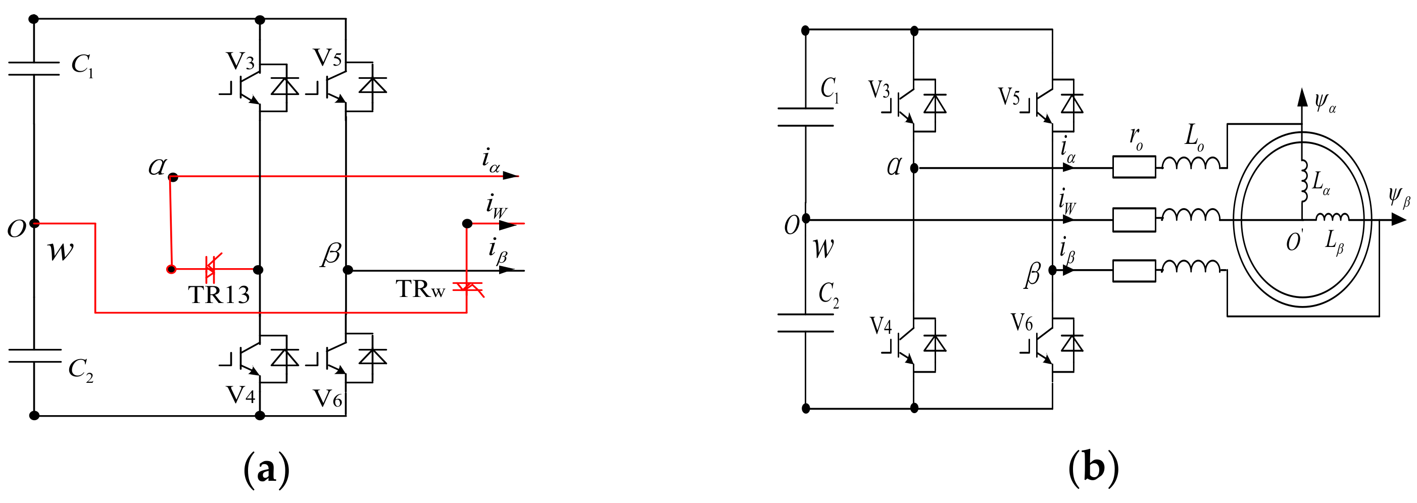
2.2. Fault Diagnosis and Reconstruction of the Back-Stage Two-Phase Quadrature Inverter

This section mainly analyzes the fault characteristics of the voltage between the midpoint potential of the arm and the midpoint potential of the DC side after the open-circuit failure of the IGBT in the subsequent two-phase quadrature inverter, that is the three-phase arm midpoint voltage u_αo, u_wo, and u_βo of the inverter in Figure 1, and use these features to diagnose faults. This section proposes a fault diagnosis algorithm based on the voltage polarity at the midpoint of the arm can realize secondary fault diagnosis.

2.2.1. The Fault Diagnosis Algorithm and Reconstruction Strategy of the Back-Stage Two-Phase Quadrature Inverter after Primary Failure

Suppose the bridge arm switch function is:

$$S_x=\left\{\begin{array}{l}1\hspace{0.33em}\hspace{0.33em}\hspace{0.33em}\hspace{0.33em}\hspace{1em}\mathrm{upper} \mathrm{bridge} \mathrm{on}\\ -1\hspace{0.33em}\hspace{0.33em}\hspace{0.33em}\hspace{0.33em}\hspace{0.33em}\mathrm{lower} \mathrm{bridge} \mathrm{on}\end{array}\right.$$

(1)

where x is one of the three phases (α, w, β). The midpoint voltage of the bridge arm can be expressed as:

$$u_{xo}=\frac{u_{dc}}{2}{S}_x$$

(2)

Take the fault of IGBT V₁ as an example. When V₁ works under normal conditions, the midpoint voltage of the bridge arm is:

$$u_{\alpha oN}=\left\{\begin{array}{l}\frac{u_{dc}}{2}\hspace{0.33em}\hspace{0.33em}\hspace{0.33em}\hspace{0.33em}\hspace{0.33em}\hspace{0.33em}\hspace{0.33em}{S}_{\alpha }=1\\ -\frac{u_{dc}}{2}\hspace{0.33em}\hspace{0.33em}\hspace{0.33em}\hspace{0.33em}\hspace{0.33em}{S}_{\alpha }=-1\end{array}\right.$$

(3)

When an open-circuit fault occurs in V₁ and S_α = 1, both V₁ and V₂ are in a disconnected state, and point α is suspended. At this time, i_α = 0 and u_αo′ = 0. The potential at point α is equivalent to the potential at point O′, that is, u_αoF = u_o′o = −u_oo′. From the circuit of the inverter in Figure 1, u_oo′ can be obtained as:

$$u_{{oo}^{\prime }}=-\frac{u_{{\omega o}^{\prime }}+u_{{\beta o}^{\prime }}}{3}=-\frac{u_{dc}}{3}\left(S_{\omega }+S_{\beta }\right)+u_{dc}$$

(4)

Then:

$$u_{\alpha oF}=-u_{{oo}^{\prime }}=\frac{u_{dc}}{3}\left(S_{\omega }+S_{\beta }\right)-u_{dc}$$

(5)

In Equation (5), u_αoF represents u_αo after failure. Substituting different values of S_w and S_β, the midpoint voltage of the α-phase arm after the fault can be obtained as:

$$u_{\alpha oF}<\frac{u_{dc}}{2}$$

(6)

Define the voltage deviation at the midpoint of the bridge arm as:

$$\Delta u_{xo}=u_{xoF}-u_{xoN}$$

(7)

Then the voltage deviation at the midpoint of the α-phase arm is:

$$\Delta u_{\alpha o}=u_{\alpha oF}-u_{\alpha oN}<0$$

(8)

Define the voltage deviation polarity at the midpoint of the bridge arm as:

$$J_{xo}=\left\{\begin{array}{l}P\begin{array}{cc}& \Delta u_{xo}>0\end{array}\\ Z\begin{array}{cc}& \Delta u_{xo}=0\end{array}\\ N\begin{array}{cc}& \Delta u_{xo}<0\end{array}\end{array}\right.$$

(9)

where P, Z, N stand for positive, zero and negative, respectively. Thus there is:

$$J_{\alpha o}=N$$

(10)

The voltage polarity at the midpoint of the α-phase arm is negative N. In other words, when V₁ has an open-circuit fault and S_α = 1, the polarity of the voltage at the midpoint of the bridge arm is negative. In the same way, the polarity of the midpoint voltage of other bridge arms can be obtained when other IGBTs fail.

In the actual engineering environment, due to various interferences on the DC side capacitors, the midpoint voltage deviation will not be exactly zero. In order to avoid misjudgment, the mid-point voltage deviation threshold Δu_th is set to eliminate the zero-point drift of the mid-point voltage deviation value, so that the polarity of the mid-point voltage deviation can be redefined as:

$$J_{xo}=\left\{\begin{array}{ll}P& \Delta u_{xo}>\Delta u_{th}\\ Z& \left|\Delta u_{xo}\right|\le \Delta u_{th}\\ N& \Delta u_{xo}<-\Delta u_{th}\end{array}\right.$$

(11)

In the above equation, P, Z, and N respectively represent the positive, zero, and negative polarity of the midpoint voltage deviation. In this article, set Δu_th as 1/10 Δu_xomax, namely u_dc/30. Only when |Δu_xo| > Δu_th, the polarity of the neutral point voltage deviation value is considered to have changed.

In

Table 1. Primary fault diagnosis.

Case	Primary Fault	Jαo	Jwo	Jβo
1	/	Z	Z	Z
2	V1	N	Z	Z
3	V2	P	Z	Z
4	V3	Z	N	Z
5	V4	Z	P	Z
6	V5	Z	Z	N
7	V6	Z	Z	P
8	V1 & V2	N/P	Z	Z
9	V1 & V3	N	N	Z
10	V1 & V4	N	P	Z
11	V1 & V5	N	Z	N
12	V1 & V6	N	Z	P
13	V2 & V3	P	N	Z
14	V2 & V4	P	P	Z
15	V2 & V5	P	Z	N
16	V2 & V6	P	Z	P
17	V3 & V4	Z	N/P	Z
18	V3 & V5	Z	N	N
19	V3 & V6	Z	N	P
20	V4 & V5	Z	P	N
21	V4 & V6	Z	P	P
22	V5 & V6	Z	Z	N/P

, if two switching tubes of the same bridge arm fail at the same time, such as V₁ & V₂, V₃ & V₄, V₅ & V₆, and if the upper tube is open, the polarity of the midpoint voltage of the bridge arm is N, and otherwise P.

When the fault is detected in V, immediately reconstruct the inverter topology: first cut off V₁, turn on TR_w and TR₁₃, stop triggering V₂, and then send the pulse signals of V₁ and V₂ to V₃ and V₄ respectively. Namely the α-phase is reconstituted by V₃ and V₄, and the DC-side capacitor as the w-phase. The reconstruction process is shown in the Figure 2.

The rest of the reconstruction status is shown in

Table 2. First reconfigurable inverter switching status.

No.	Primary Fault	Connection	First Reconstruction
0	/	TRb	/
1	V1	TRw & TR13	Sα (V3, V4) Sw (C1, C2)
2	V2	TRw & TR13	Sα (V3, V4) Sw (C1, C2)
3	V3	TRw	Sw (C1, C2)
4	V4	TRw	Sw (C1, C2)
5	V5	TRw & TR35	Sβ (V3, V4) Sw (C1, C2)
6	V6	TRw & TR35	Sβ (V3, V4) Sw (C1, C2)
7	V1 & V2	TRw & TR13	Sα (V3, V4) Sw (C1, C2)
8	V3 & V4	TRw	Sw (C1, C2)
9	V5 & V6	TRw & TR35	Sβ (V3, V4) Sw (C1, C2)
18	V1 & V4	TRw & TR13	Sα(V3, V2) Sw (C1, C2)
19	V2 & V3	TRw & TR13	Sα(V1, V4) Sw (C1, C2)
20	V3 & V6	TRw & TR35	Sβ(V5, V4) Sw (C1, C2)
21	V4 & V5	TRw & TR35	Sβ(V3, V6) Sw (C1, C2)

. It can be seen from Table 2 that no matter which IGBT is reconstructed after failure, it can be reconstructed to the structure shown in Figure 2b, and the w-phase is always replaced by the DC side capacitors.

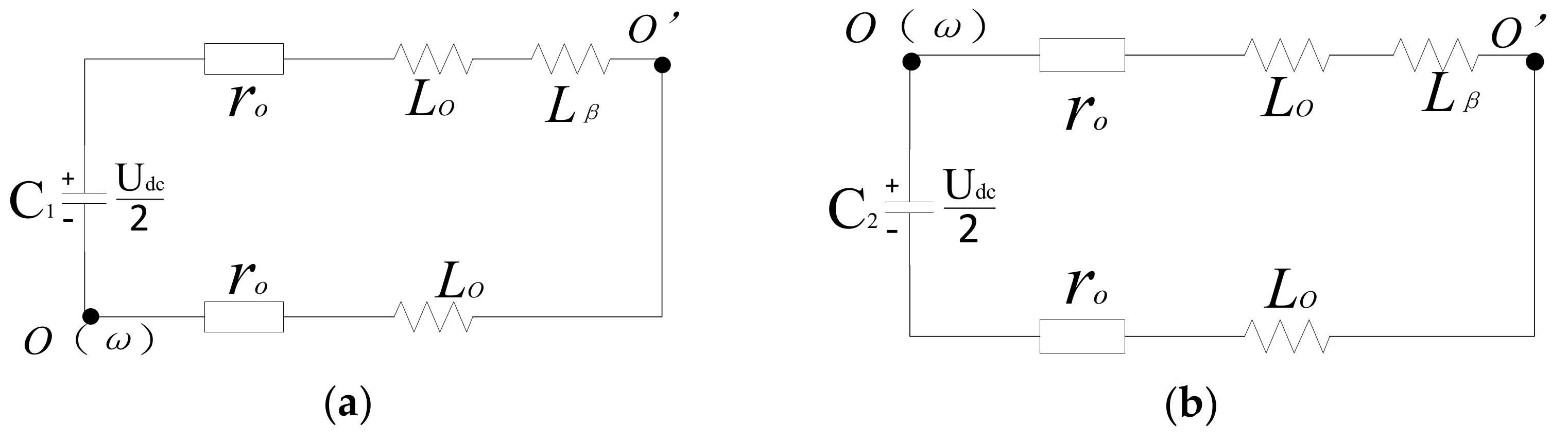
2.2.2. The Fault Diagnosis Algorithm and Reconstruction Strategy after the Secondary Fault of the Back-Stage Two-Phase Quadrature Inverter

The inverter is reconstructed after primary failure, so that the inverter can work in fault-tolerant conditions. It can be seen from Table 1 that some IGBTs can be used for reconstruction after some faults have occurred. Take case 2 in Table 1 as an example, when the fault of V₁ is removed, V₂ is still normal. Therefore, when a secondary failure occurs in the inverter, V₂ can be used for secondary reconstruction.

Firstly, perform a secondary fault diagnosis on the inverter after the first reconstruction shown in Figure 2b. Take the IGBT V₄ failure as an example. V₃ and V₄ construct α-phase in the first reconstruction, so the midpoint voltage of the arm also satisfies Equation (2). Similarly, when V₄ has an open-circuit fault and S_α= 1, both V₃ and V₄ are in a disconnected state, and the α point is suspended. Besides, i_α = 0 and u_αo′ = 0. The potential at point α is equivalent to the potential at point O′, that is, u_αoF = u_o′o = −u_oo′. when S_α= −1, the equivalent circuit is shown in Figure 3.

From Figure 3a, we can obtain:

$$u_{o^{\prime }o}=\frac{u_{dc}}{4}\times \frac{r_o+L_o}{2\left(r_o+L_o\right)+L_{\beta }}$$

(12)

The r_o is the inner resistance of the inductance L_o. The midpoint voltage deviation of α-phase is:

$$\Delta u_{\alpha o}=\frac{u_{dc}}{4}\times \frac{r_o+L_o}{2\left(r_o+L_o\right)+L_{\beta }}+\frac{u_{dc}}{2}>0$$

(13)

The polarity of the midpoint voltage deviation is:

$$J_{\alpha o}=J\left[\Delta u_{\alpha o}\right]=P$$

(14)

From Figure 3b, we can get:

$$u_{o^{\prime }o}=\frac{u_{dc}}{4}\times \frac{r_o+L_o+L_{\beta }}{2\left(r_o+L_o\right)+L_{\beta }}$$

(15)

The voltage deviation at the midpoint is:

$$u_{o^{\prime }o}-u_{\alpha oN}=\frac{u_{dc}}{2}\left(1-\frac{r_o+L_o+L_{\beta }}{4\left(r_o+L_o\right)+2L_{\beta }}\right)>0$$

(16)

The polarity of the midpoint voltage deviation is also positive. That is, when the fault occurs in V₄, no matter whether S_β = 1 or S_β = −1, there will be $J_{\alpha o}=P$.

In the same way, the polarity of the voltage deviation at the midpoint of the other arms can be obtained when other IGBTs fail. The secondary fault diagnosis is shown in

Table 3. Secondary fault diagnosis.

Case	Primary Fault	Secondary Fault	Jαo	Jβo
1	V1	V4	P	Z
2	V1	V6	Z	P
3	V2	V3	N	Z
4	V2	V5	Z	N
5	V3	V2	P	Z
6	V3	V6	Z	P
7	V4	V1	N	Z
8	V4	V5	Z	N
9	V5	V2	P	P
10	V5	V4	P	Z
11	V6	V1	N	Z
12	V6	V3	N	Z

.

It can be seen from the reasoning process that the secondary fault diagnosis method is the same as the fault diagnosis method for the primary fault. The fault diagnosis method based on the voltage polarity at the midpoint of the bridge arm can be applied to the secondary fault diagnosis after the primary fault occurring in inverter and reconfiguration, which has the characteristic of strong versatility.

When the fault is detected in V₄, the inverter topology is immediately reconstructed for the second time: V₄ is cut off, TR_w and TR₁₃ are kept connected, and V₂ is triggered. Namely α-phase is reconstructed by V₃ and V₂, and the DC side capacitor remains as the w-phase. The reconstruction result is shown in the Figure 4. The rest of the reconstruction status is shown in

Table 4. Secondary reconfigurable inverter switching status.

Case	Primary Fault	Connection	Secondary Fault	Secondary Construction
1	V1	TRw & TR13	V4	Sα (V3, V2)
2	V2	TRw & TR13	V3	Sα (V1, V4)
3	V3	TRw & TR13	V2	Sα (V1, V4)
4	V3	TRw & TR35	V6	Sβ (V5, V4)
5	V4	TRw & TR13	V1	Sα (V3, V2)
6	V4	TRw & TR35	V5	Sβ (V3, V6)
7	V5	TRw & TR35	V4	Sβ (V3, V6)
8	V6	TRw & TR35	V3	Sβ (V5, V4)

.

It can be seen from Table 4 that after some switching tubes are reconstructed after failure, the second reconstruction can also be carried out into the topology shown in Figure 2b, and the w-phase is always reconstructed by the DC side capacitor. And this structure ensures that the stirring effect of the important two-phase α-phase and β-phase of the electromagnetic stirrer is not affected.

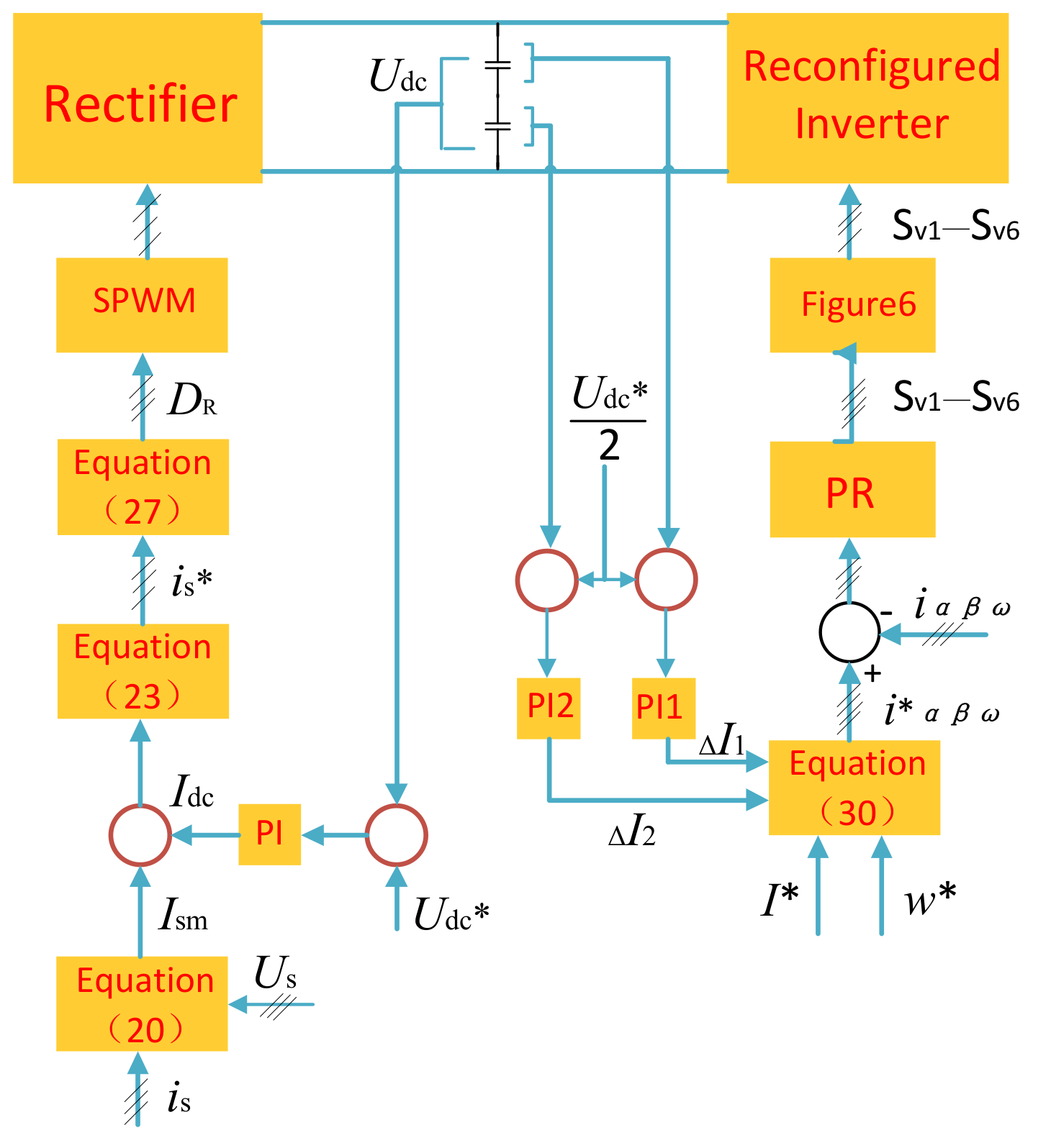
2.3. Fault-Tolerant Control Strategy

The control goal of the front-stage rectifier is to achieve the stability of the total DC side voltage of the two series DC capacitors. Due to the existence of the common arm in the back-stage inverter, the change of output power leads to the change of the instantaneous power of the DC side capacitor all the time. DC side voltage is not a constant value, but there are certain fluctuations that need to be suppressed. The goal of the back-stage inverter control is to achieve equal voltage on the two DC sides and make the inverter output current equal to the current reference value. And when the inverter is converted from the normal working state to the fault-tolerant working state, there is no need to change the control method.

For the front-stage rectifier, the grid voltage is:

$$\left\{\begin{array}{l}{u}_{sa}=U_{sm}\sin \left({\omega }_{0}t\right)\\ u_{sb}=U_{sm}\sin \left({\omega }_{0}t-\frac{2\pi }{3}\right)\\ u_{sc}=U_{sm}\sin \left({\omega }_{0}t+\frac{2\pi }{3}\right)\end{array}\right.$$

(17)

where ω₀ is an angular frequency with a frequency of 50 Hz. The measured grid current is i_sa, i_sb and i_sc. Then the apparent power P_s on the grid side is:

$$P_s=u_{sa}{i}_{sa}+u_{sb}{i}_{sb}+u_{sc}{i}_{sc}$$

(18)

The apparent power P_s on the grid side can also be expressed as:

$$P_s=\frac{3U_{sm}}{2}{I}_{sm}$$

(19)

where I_sm is the magnitude of the grid current, then I_sm is:

$$I_{sm}=\frac{2P_s}{3U_{sm}}$$

(20)

As a load, the operating condition of the electromagnetic stirrer is forward stirring-stop-reverse stirring. Its power is constantly changing, which causes voltage fluctuations on the DC side. Use the feedforward PI control to control the fluctuation of the DC side voltage, and we can get:

$$\Delta I_{dc}=k_p\left(u_{dc}{}^{*}-u_{dc}\right)+k_i{\displaystyle {\int }_{Ts}\left(u_{dc}{}^{*}-u_{dc}\right)dt}$$

(21)

where k_p is the proportionality coefficient and k_i is integral coefficient for the PI control. Then the magnitude of the grid reference current is:

$$I_{sm}{}^{*}=I_{sm}+\Delta I_{dc}$$

(22)

The reference current of the grid is:

$$\left\{\begin{array}{l}{i}_{sa}^{*}=I_{sm}^{*}\sin \left(\omega t\right)\\ i_{sb}^{*}=I_{sm}^{*}\sin \left(\omega t-\frac{2\pi }{3}\right)\\ i_{sc}^{*}=I_{sm}^{*}\sin \left(\omega t+\frac{2\pi }{3}\right)\end{array}\right.$$

(23)

According to Figure 1, the output voltage of the front-stage rectifier can be expressed as:

$$\left\{\begin{array}{l}{u}_{Ra}=u_{sa}-L_s\frac{d{i}_{sa}}{dt}=u_{dc}{D}_{Ra}\\ u_{Rb}=u_{sb}-L_s\frac{d{i}_{sb}}{dt}=u_{dc}{D}_{Rb}\\ u_{Rc}=u_{sc}-L_s\frac{d{i}_{sc}}{dt}=u_{dc}{D}_{Rc}\end{array}\right.$$

(24)

where D_Rx is the modulating switch signal, and x = (a, b, c). Discretize Equation (24) to get:

$$\left\{\begin{array}{l}{u}_{sa}\left(k\right)-L_s\frac{i_{sa}\left(k+1\right)-i_{sa}\left(k\right)}{T_s}=u_{dc}\left(k\right)D_{Ra}\left(k\right)\\ u_{sb}\left(k\right)-L_s\frac{i_{sb}\left(k+1\right)-i_{sb}\left(k\right)}{T_s}=u_{dc}\left(k\right)D_{Rb}\left(k\right)\\ u_{sc}\left(k\right)-L_s\frac{i_{sc}\left(k+1\right)-i_{sc}\left(k\right)}{T_s}=u_{dc}\left(k\right)D_{Rc}\left(k\right)\end{array}\right.$$

(25)

where, T_s is the switching period of the IGBT. Take the grid reference current as the sampling current value of the (k + 1)th switching cycle, namely:

$$\left\{\begin{array}{l}{i}_{sa}\left(k+1\right)=i_{sa}^{*}\\ i_{sb}\left(k+1\right)=i_{sb}^{*}\\ i_{sc}\left(k+1\right)=i_{sc}^{*}\end{array}\right.$$

(26)

According to Equation (26), we can get:

$$\left\{\begin{array}{l}{D}_{Ra}\left(k\right)=\frac{1}{u_{dc}\left(k\right)}\left\{u_{sa}\left(k\right)-\frac{L_s}{T_s}\left[i_{sa}^{*}\left(k\right)-i_{sa}\left(k\right)\right]\right\}\\ D_{Rb}\left(k\right)=\frac{1}{u_{dc}\left(k\right)}\left\{u_{sb}\left(k\right)-\frac{L_s}{T_s}\left[i_{sb}^{*}\left(k\right)-i_{sb}\left(k\right)\right]\right\}\\ D_{Rc}\left(k\right)=\frac{1}{u_{dc}\left(k\right)}\left\{u_{sc}\left(k\right)-\frac{L_s}{T_s}\left[i_{sc}^{*}\left(k\right)-i_{sc}\left(k\right)\right]\right\}\end{array}\right.$$

(27)

Send the three-phase modulation signal obtained by Equation (27) to the PWM modulation unit, then we can get the output of the switching drive signal of the rectifier, and the IGBT is driven to output the desired voltage and current. In this way, a composite control method of feedforward control and feedback control is formed, which effectively combines the fast response speed of feedforward control and the closed-loop tracking characteristics of feedback, and realizes the stability of the total DC side voltage. And the three-phase input current is sine wave and with high power factor, which provides high-quality DC voltage for the back-stage inverter. In the control strategy of the back-stage inverter, it is necessary to realize the tracking of the given current and the voltage equalization of the DC side capacitances.

First, compare the detected voltages on the two DC capacitors with the given DC side voltages, and we can obtain:

$$\Delta I_1=k_{p1}+k_{i1}{\displaystyle \int \left(\frac{u_{dc}^{*}}{2}-u_{dc1}\right)dt}$$

(28)

$$\Delta I_2=k_{p2}+k_{i2}{\displaystyle \int \left(\frac{u_{dc}^{*}}{2}-u_{dc2}\right)dt}$$

(29)

k_p1 is the proportionality coefficient and k_i1 is integral coefficient for the PI1 controller. k_p2 is the proportionality coefficient and k_i2 is integral coefficient for the PI2 controller. The amplitude of the output current of the electromagnetic stirring power supply specified by the user is I*, and the frequency is ω*. Therefore, the corrected given current amplitude is:

$$I_m=I^{*}-\Delta I_1-\Delta I_2$$

(30)

The given current is:

$$\left\{\begin{array}{l}{i}_{\alpha }{}^{*}=I_m\sin \left({\omega }^{*}t\right)\\ i_{\beta }{}^{*}=I_m\sin \left({\omega }^{*}t-\frac{\pi }{2}\right)\\ i_{\omega }{}^{*}=-i_{\alpha }^{*}-i_{\beta }^{*}\end{array}\right.$$

(31)

Perform PR control on the difference between the detected output current of the electromagnetic stirrer and the given current to obtain a modulation signal, and perform SPWM modulation on the modulation signal to obtain 6 pulse signals. Finally, after resetting the fault-tolerant pulse, the final pulse signals of the 6 IGBTs are obtained.

The overall control process of the electromagnetic stirring system is shown in Figure 5.

The fault-tolerant pulse reset rule in the above figure is shown in Figure 6. The red dashed box in the figure is the pulse reset required for reconstruction after primary failure, corresponding to case 1–21 in Table 2. The blue dashed box is the pulse reset required for reconstruction after secondary failure, corresponding to case 1–8 in Table 4. Take case1 of the first failure as an example: if the α-phase IGBT V₁ fails, V₃ and V₄ will be reconstructed into the α-phase, and the two capacitors on the DC side will form the w-phase. At the same time, in the control algorithm, the original pulse signals of V₁ and V₂ are reset to V₃ and V₄ respectively, that is, S_V3 = S_V1, S_V4 = S_V2. There is no need to change the control method, and the topology of the back-stage inverter is still maintained in a normal working state after reconstruction.

3. Results and Discussion

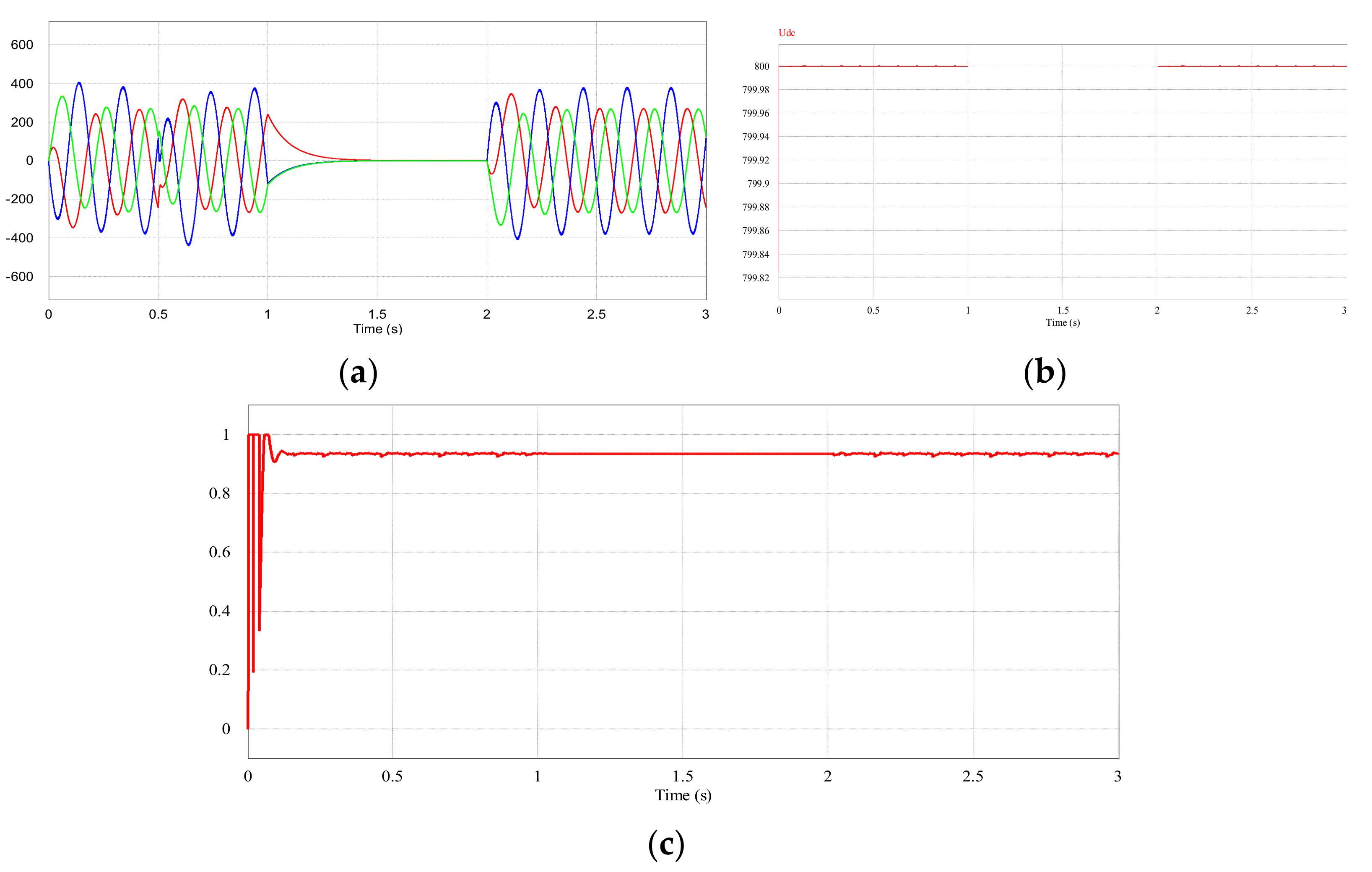
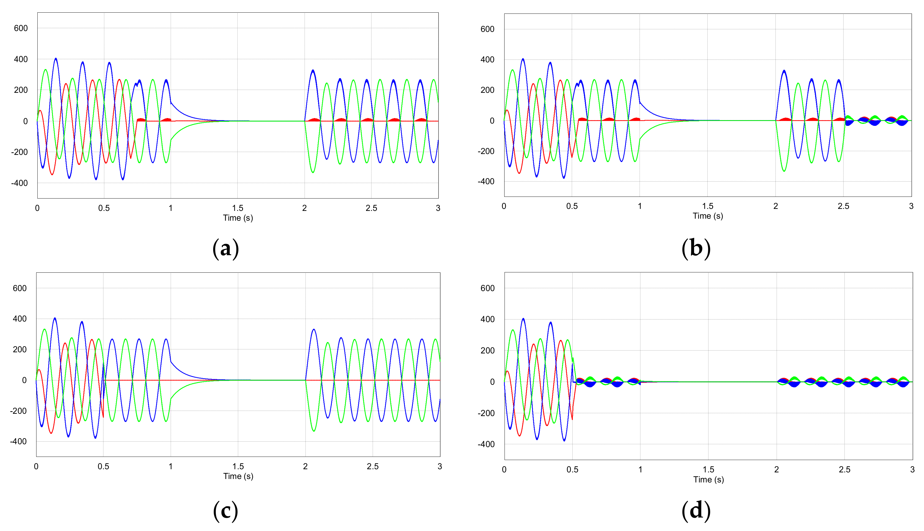
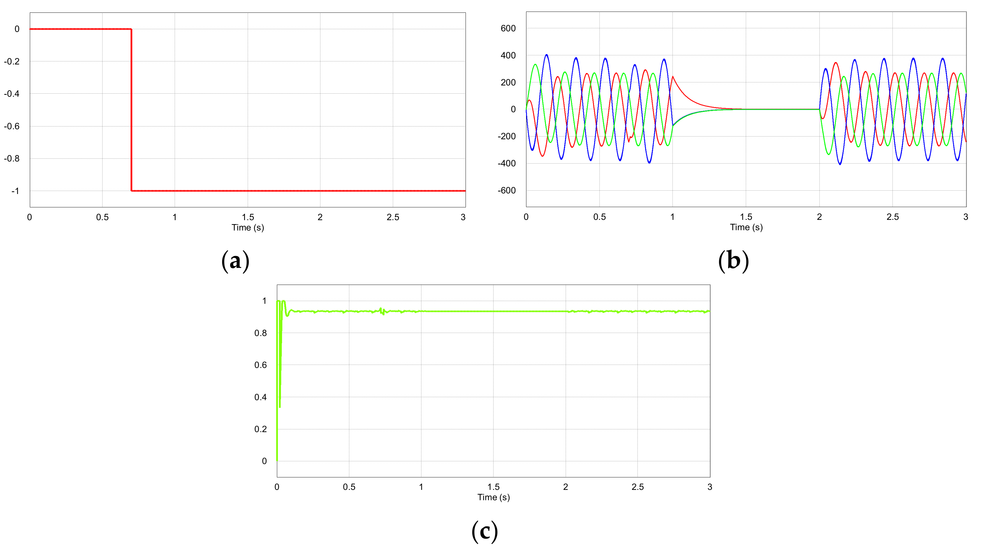
3.1. Simulation and Analysis

In order to verify the correctness and effectiveness of the reconstructing main circuit topology and the control strategy of the high-reliability electromagnetic stirring power supply presented in this paper, the proposed topology is modeled on PSim and simulation experiments are performed. When the system is running normally, the simulation circuit model is shown in Figure 1. The grid voltage is 380 V, 50 Hz. The filter inductance on the grid side is 0.5 mH. The DC side capacitance value is 5000 μF. The DC side voltage is 800 V. The inverter output side filter is 1 mH. The equivalent inductance of the electromagnetic stirrer is 10 mH, and the equivalent resistance is 0.1 Ω. In the working process of the electromagnetic stirrer, it usually runs in three working states of forward rotation, stop, and reverse rotation.

When the electromagnetic stirring power supply works normally, the output currents, DC side output voltage and the power factor of the electromagnetic stirring power supply are shown in Figure 7.

From the Figure 7, if the electromagnetic stirring power supply works normally, the output currents are good sine waves. The amplitudes of phase α and phase β are same, and the phase angle is 90 degrees between the two phases. The amplitude of phase w is greater because there is no inductance. The DC side voltage is stable at 800 V. The power factor keeps the value 0.93.

If the current system does not have the reconstruction topology shown in the yellow box in Figure 1, and the simulation results of the failures of the back-stage inverter are shown in Figure 8.

Four different faulty conditions are done without the proposed reconstruction topology in the paper. The single switch V₁ faults at t = 0.7 s. The two switches V₁ and V₄ are at t = 0.5 s for the first fault and t = 2.5 s for the second fault, respectively. Both V₁ and V₂ in the same bridge are faulty at t = 0.5 s. Both V₁ and V₄ in the different bridge are faulty at t = 0.5 s. The output currents of the back-stage inverter cannot get the correct waveform in above faulty conditions. The system cannot work normally if the power system does not have the reconstruction topology.

The proposed reconstructed topology of the system is shown in the yellow box in Figure 1. The simulation results in four different fault conditions with the proposed reconstructed topology are shown in Figure 9 for single faulty switch, Figure 10 for second fault, Figure 11 for two fault switches in the same bridge, and Figure 12 for two fault switches in different bridges.

The single switch V₁ faults at t = 0.7 s in Figure 9. The switch V₁ is at t = 0.5 s for the first fault and switch V₄ at t = 2.5 s for the second fault, respectively, in Figure 10. Both V₁ and V₂ in the same bridge are faulty at t = 0.5 s in Figure 11. Both V₁ and V₄ in the different bridge are faulty at t = 0.5 s in Figure 12. The output currents of the back-stage inverter cannot get the correct waveform in above faulty conditions. It can be seen from these figures that different faults are diagnosed correctly. The output current waveforms can track the given current waveforms and can keep good shapes before and after the fault through transient vibration of about 0.01 s. The power factors can be maintained stable before and after the fault. All waveforms are almost the same as Figure 7. The waveforms of the DC side voltage in different faulty conditions are the same as Figure 7b, which are not shown here in order to avoid repetition.

From all the simulation results, we can obtain that the electromagnetic stirring power supply reconstructed topology proposed in this paper can maintain the normal operation of the system when the back-stage inverter fails. It verifies the validity of the fault diagnosis algorithm proposed in this paper, the correctness of the reconstructed topology, and the fault tolerant control strategy.

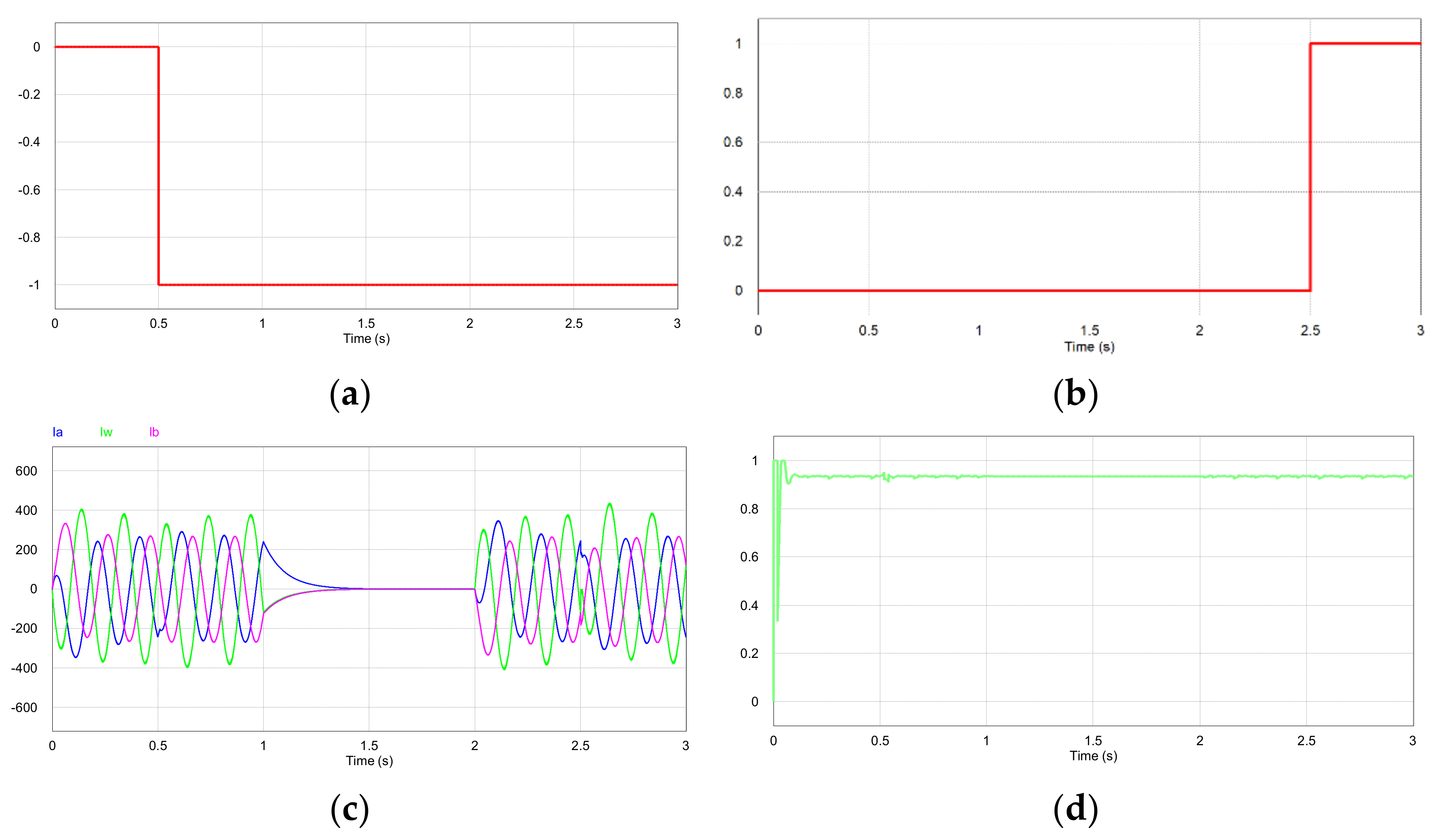
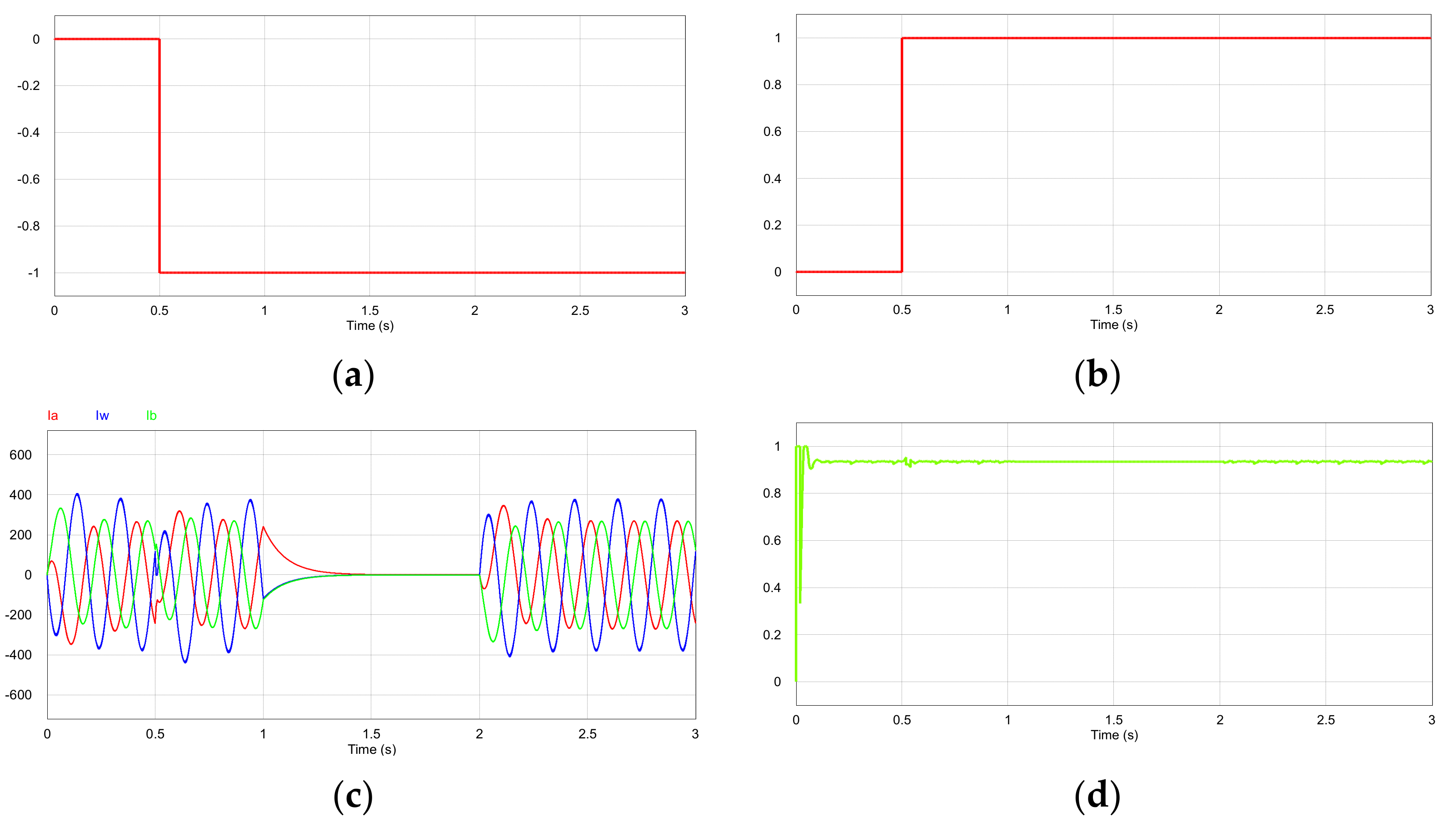
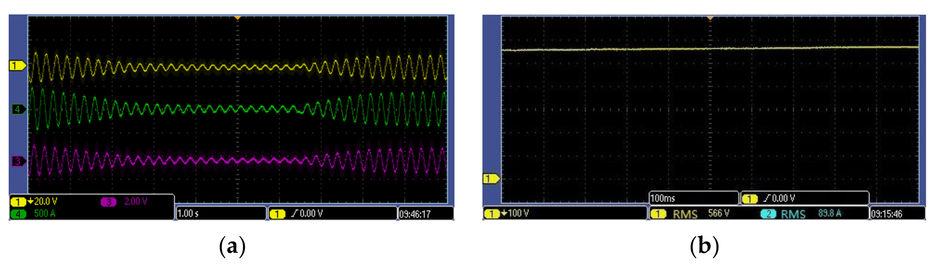
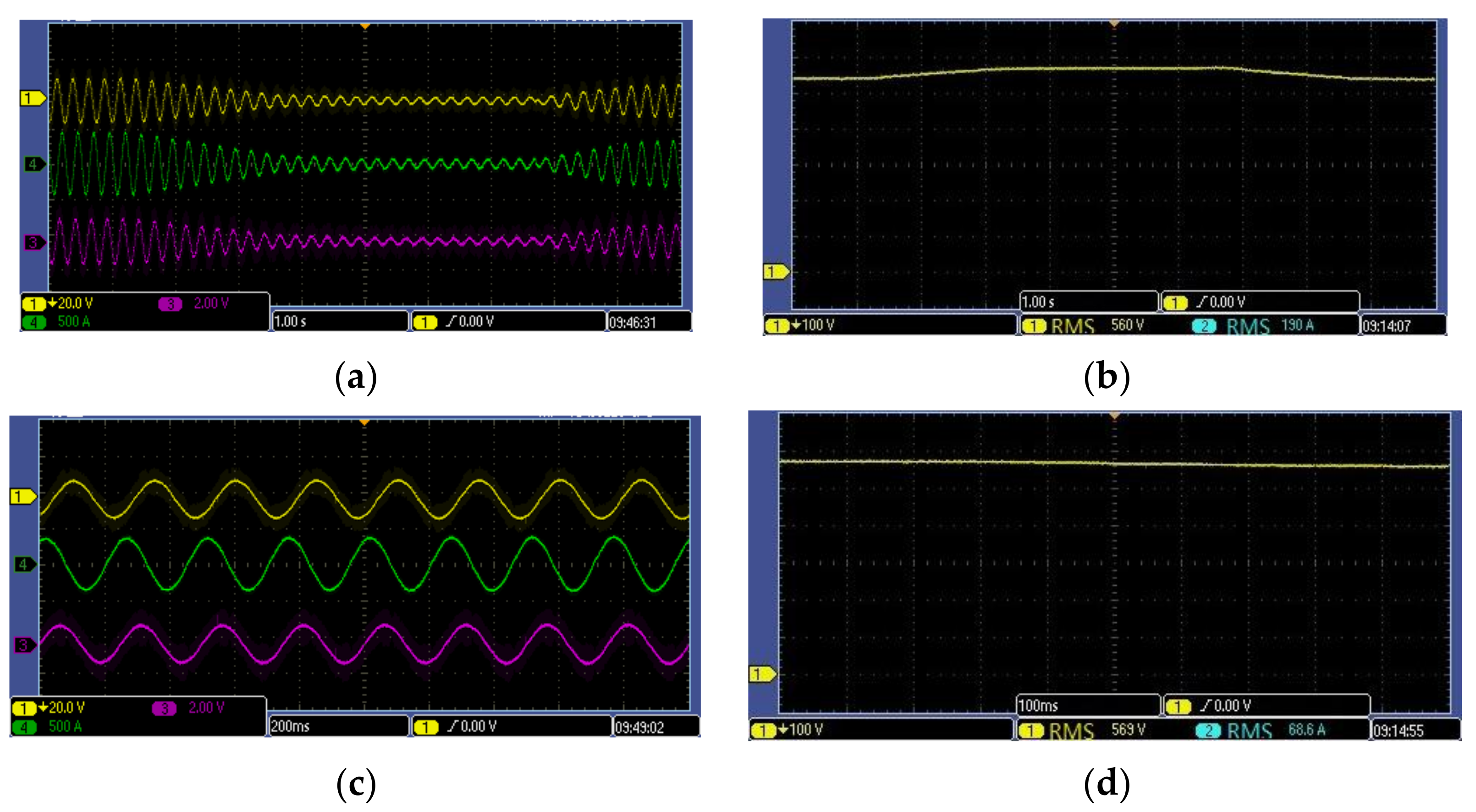
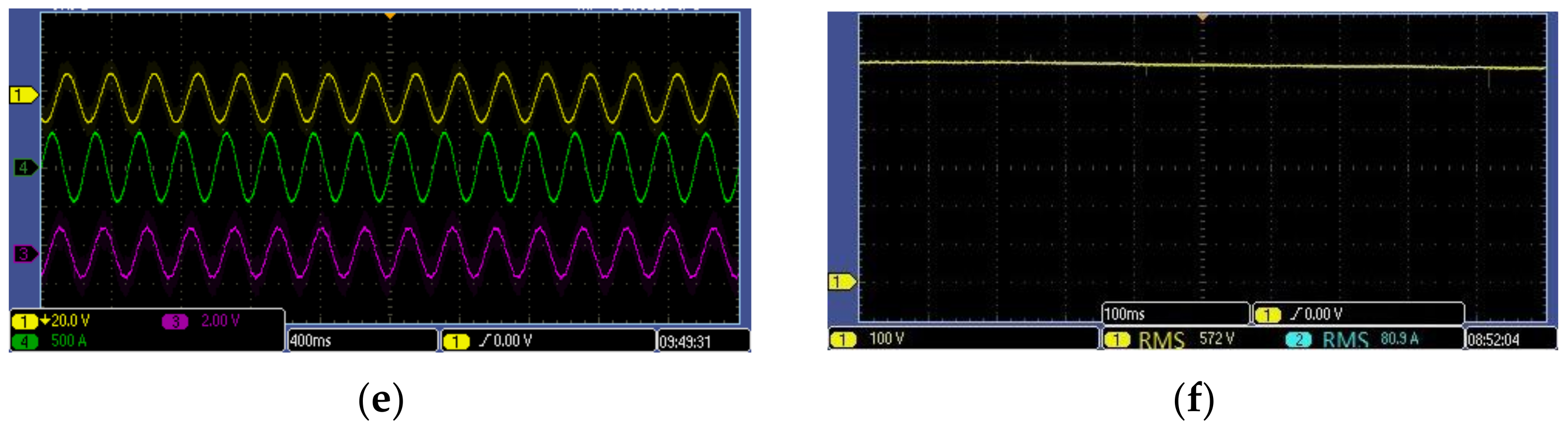
3.2. Experiment and Analysis

The reconstructed topology of high-reliability electromagnetic stirring power supply and the control algorithm are applied to the electromagnetic stirrer for experiments. The grid voltage is 380 V, 50 Hz. The filter inductance on the grid side is 1 mH. The DC side capacitance value is 5000 μF. The DC side voltage is 400 V. The inverter output side filter is 0.5 mH. The equivalent inductance of the electromagnetic stirrer is 50 mH, and the equivalent resistance is 0.5 Ω. This article uses Case 2 in Table 1 as an example for experimental verification. The experimental results are shown in Figure 13, Figure 14, Figure 15.

Figure 13a,b are the waveforms of three-phase output currents and the corresponding DC side voltage of the normal working conditions for the forward-stop-reverse operation. The three-phase output currents are completely consistent with the given currents, and the DC side voltage is stable without fluctuations. Figure 14a,b are the waveforms of α-phase output current and the corresponding DC side voltage of the fault working conditions without reconstructed topology for the forward-stop-reverse operation. The output current is distorted, and the amplitude and phase of the given current waveform cannot be tracked at all, and the DC side voltage also fluctuates. Figure 15a–f are the waveforms of the three-phase output currents and the corresponding DC side voltage of the fault working conditions and reconstructed topology for the forward-stop-reverse operation, the three-phase output current and the corresponding DC side voltage for forward running condition, the three-phase output current and the corresponding DC side voltage for reverse working operation. From Figure 15a–f, it can be seen that, regardless of whether the electromagnetic stirrer is agitated forward or reversely, the three-phase output currents of the inverter can be consistent with normal operation, which can maintain a smooth sine wave and correctly follow the given currents. The DC side voltage remains stable. Therefore, the problem of stable control of the high-reliability electromagnetic stirring power supply is solved. The switching of forward-stop or stop-reverse stirring can be maintained fast. The experimental results verify the validity of the fault diagnosis algorithm, the correctness of the reconstructed topology and the fault-tolerant control strategy proposed in this paper.

4. Conclusions

This paper proposes a fault diagnosis algorithm, reconstructed topology and its fault-tolerant control strategy for a high-reliability electromagnetic stirring power supply, which is applied to electromagnetic stirrers. The high-reliability electromagnetic stirring power supply includes a front-stage rectifier and a back-stage reconstructed inverter. When a fault occurs in IGBT in the back-stage reconstructed inverter, the fault diagnosis algorithm locates the fault switch and removes the faulty IGBT while the inverter is reconstructed to keep the system running continuously. The system can realize both fault diagnosis and reconstruction twice. A pulse reset method combined with the control method of the back-stage inverter for the purpose of forming a fault-tolerant control strategy is proposed, so the high-reliability electromagnetic stirring power supply does not need to switch the control algorithm before and after the failure. The reliability of the electromagnetic stirring power supply is improved from the control algorithm. Moreover, it ensures the ability of quick tracking currents of the system and the reliable and stable operation of the device. Finally, simulations and experiments verify the validity of the fault diagnosis algorithm, the correctness of the reconstructed topology and the fault-tolerant control strategy proposed in this paper.

References

1. Otake, R.; Yamada, T. Effects of Double-Axis Electromagnetic Stirring in Continuous Casting. IEEE Trans. Magn. 2008, 44, 4517–4520. [Google Scholar] [CrossRef]
2. Liu, C.-T. Refined Model Development and Performance Assessment of a Linear Induction-Type Electromagnetic Stirrer. IEEE Trans. Magn. 2010, 46, 3724–3730. [Google Scholar] [CrossRef]
3. Ege, Y.; Kalender, O. Electromagnetic Stirrer Operating in Double Axis. IRE Trans. Ind. Electron. 2010, 57, 2444–2453. [Google Scholar]
4. Liu, C.-T.; Lin, C.-D.; Lee, W.-J.; Chen, J.-H. Electromagnetic stirring systems. IEEE Ind. Appl. Mag. 2011, 46, 38–43. [Google Scholar]
5. Mao, B.; Zhang, G.; Li, A. Theory and Technology of Electromagnetic Stirring for Continuous Casting Steel. Metallurgical Industry Press: Beijing, China, 2012. [Google Scholar]
6. Luo, A.; Xiao, H.; Ouyang, H.; Wu, C.; Ma, F.; Shuai, Z. Development and Application of the Two-Phase Orthogonal Power Supply for Electromagnetic Stirring. IEEE Trans. Power Electron. 2013, 28, 3438–3446. [Google Scholar] [CrossRef]
7. Li, Y. Electromagnetic stirring power supply system with bidirectional energy flow and its control strategy. In Proceedings of the Power Electronics and Applications (EPE’17 ECCE Europe), Warsaw, Poland, 11–14 September 2017. [Google Scholar]
8. Rojat, G.; Mertz, J.; Foggia, A. Theoretical and Experimental Analysis of a Two-Phase Inverter-Fed Induction Motor. IEEE Trans. Ind. Appl. 1969, 15, 601–605. [Google Scholar]
9. Collins, E.R.; Puttgen, H.B.; Sayle, W.E. Single-phase induction motor adjustable speed drive: Direct phase angle control of the auxiliary winding supply. In Proceedings of the 1988 IEEE Industry Applications Society Annual Meeting, Pittsburgh, PA, USA, 2–7 October 1988. [Google Scholar]
10. Young, C.M.; Liu, C.C.; Liu, C.H. New inverter-driven design and control method for two-phase induction motor drives. Proc. Electr. Power Appl. 1996, 143, 458–466. [Google Scholar] [CrossRef]
11. Jang, D.H.; Yoon, D.Y. Space-vector PWM technique for two-phase inverterfed two-phase induction motors. In Proceedings of the 1999 IEEE Industry Applications Conference, Phoenix, AZ, USA, 3–7 October 1988. [Google Scholar]
12. Jabbar, M.A.; Khambadkone, A.M.; Zhang, Y. Space-vector Modulation in a two-phase induction motor drive for constant-power operation. IRE Trans. Ind. Electron. 2004, 51, 1081–1088. [Google Scholar] [CrossRef]
13. Rajaei, A.H.; Mohamadian, M. Single-phase induction motor drive system using z-source inverter. IET Electr. Power Appl. 2010, 4, 17–25. [Google Scholar] [CrossRef]
14. Bartholet, M.T.; Nussbaumer, T.; Kolar, J.W. Comparison of Voltage-Source Inverter Topologies for Two-Phase Bearingless Slice Motors. IRE Trans. Ind. Electron. 2011, 58, 1921–1925. [Google Scholar]
15. Wang, L.; Gao, H.; Zou, G. Modeling methodology and fault simulation of distribution networks integrated with inverter-based DG. Prot. Control. Mod. Power Syst. 2017, 2, 370–378. [Google Scholar]
16. Noureldeen, O.; Hamdan, I. A novel controllable crowbar based on fault type protection technique for DFIG wind energy conversion system using adaptive neuro-fuzzy inference system. Prot. Control. Mod. Power Syst. 2018, 3, 328–339. [Google Scholar]
17. Huang, K.; Liu, J.; Huang, S. Converters open-circuit fault diagnosis methods research for direct—driven permanent magnet wind power system. Trans. China Electrotech. Soc. 2015, 30, 129–136. [Google Scholar]
18. dos Santos, E.C., Jr.; Jacobina, C.B.; Dias, A.A.; Rocha, N. Fault tolerant ac-dc-ac single-phase to three-phase converter. IET Power Electron. 2011, 4, 1023–1031. [Google Scholar]
19. Zhang, F.; Mu, L. New protection scheme for internal fault of multi-microgrid. Prot. Control. Mod. Power Syst. 2019, 4, 159–170. [Google Scholar] [CrossRef]
20. Nair, D.V.; Murty, M. Reconfigurable control as actuator fault-tolerant control design for power oscillation damping. Prot. Control. Mod. Power Syst. 2020, 5, 70–81. [Google Scholar] [CrossRef]
21. Errabelli, R.R.; Mutschler, P. Fault-tolerant voltage source inverter for permanent magnet drives. IEEE Trans. Power Electron. 2012, 27, 500–508. [Google Scholar] [CrossRef]
22. Munim, W.N.W.A.; Duran, M.J.; Che, H.S.; Bermudez, M.; GonzalezPrieto, I.; Rahim, N.A. A unified analysis of the fault tolerance capability in six-phase induction motor drives. IEEE Trans. Power Electron. 2017, 32, 7834–7836. [Google Scholar] [CrossRef]
23. Abdel-Khalik, A.S.; Hamad, M.S.; Massoud, A.M.; Ahmed, S. Postfault operation of a nine-phase six-terminal induction machine under single open-line fault. IEEE Trans. Ind. Electron. 2018, 65, 1084–1096. [Google Scholar]
24. Xia, Y.; Gou, B.; Xu, Y. A new ensemble-based classifier for IGBT open-circuit fault diagnosis in three-phase PWM converter. Prot. Control. Mod. Power Syst. 2018, 3, 364–372. [Google Scholar]
25. Dhople, S.V.; Davoudi, A.; Domínguez-García, A.D.; Chapman, P.L. A unified approach to reliability assessment of multiphase DC–DC converters in photovoltaic energy conversion systems. IEEE Trans. Power Electron. 2012, 27, 739–751. [Google Scholar] [CrossRef]
26. Pradeep Kumar, V.V.S.P.; Fernandes, B.G. A Fault-Tolerant Single-Phase Grid-Connected Inverter Topology With Enhanced Reliability for Solar PV Applications. IEEE J. Emerg. Sel. Top. Power Electron. 2017, 5, 1254–1263. [Google Scholar]
Figure 1. The structure of the electromagnetic stirring power supply.
Applsci 11 09874 g001
Figure 2. Inverter reconstruction process when the fault occurs in V1. (a) Switching process; (b) Reconstruction result.
Applsci 11 09874 g002
Figure 3. Equivalent circuit diagram. (a) Sβ= 1; (b) Sβ= −1.
Applsci 11 09874 g003
Figure 4. Inverter reconstruction process when V4 fails. (a) Switching process; (b) Reconstruction result.
Applsci 11 09874 g004
Figure 5. Overall control block diagram.
Applsci 11 09874 g005
Figure 6. Reset rules of fault-tolerant pulse.
Applsci 11 09874 g006
Figure 7. Simulation results under the normal operation of electromagnetic stirring power supply. (a) Output currents; (b) DC side voltage; (c) power factor.
Applsci 11 09874 g007
Figure 8. Output currents of electromagnetic stirring power supply without fault tolerance. (a) faulty V1 at t = 0.7 s; (b) faulty V1 at t = 0.5 s and faulty V4 at t = 2.5 s; (c) both faulty V1 at t = 0.5 s and faulty V2 at t = 0.5 s; (d) faulty V1 at t = 0.5 s and faulty V4 at t = 0.5 s.
Applsci 11 09874 g008
Figure 9. Faulty V1 at t = 0.7 s. (a) faulty signal of V1; (b) Output currents; (c) power factor.
Applsci 11 09874 g009
Figure 10. Faulty V1 at t = 0.5 s and faulty V4 at t = 2.5 s. (a) faulty signal of V1; (b) faulty signal of V4; (c) Output currents; (d) power factor.
Applsci 11 09874 g010
Figure 11. Faulty V1 and V2 at t = 0.5 s. (a) faulty signal of V1; (b) faulty signal of V2; (c) Output currents; (d) power factor.
Applsci 11 09874 g011
Figure 12. Faulty V1 and V4 at t = 0.5 s. (a) faulty signal of V1; (b) faulty signal of V2; (c) Output currents; (d) power factor.
Applsci 11 09874 g012
Figure 13. Experimental results in the normal operation. (a) the output currents; (b) the DC side voltage.
Applsci 11 09874 g013
Figure 14. Experimental results in the faulty operation without reconstructing topology. (a) the output currents; (b) the DC side voltage.
Applsci 11 09874 g014
Figure 15. Experimental results in the faulty operation with reconstructing topology. (a) the output currents; (b) the DC-side voltage ; (c) the output currents in the forward operation; (d) the DC-side voltage in the forward operation; (e) the output currents in the reverse operation; (f) the DC-side voltage in the reverse operation.
Applsci 11 09874 g015aApplsci 11 09874 g015b