Abstract
Flow characteristics and pollutant dispersion characteristics of a mechanical upper vent of a tunnel under various discharge patterns and ambient wind were studied by using the computational fluid dynamics (CFD) numerical method and an experimental model. On this basis, variations in the environmental impact radius rcriti changing with the ambient wind velocity U for pollutants from vertical and horizontal outlets were also analyzed with the set discharge capacity. According to our findings, the pollutant emission of the upper vent under a vertical discharge pattern can be considered as free buoyant jet diffusion under the impact of the momentum of ambient wind, while the emission under the horizontal discharge pattern can be regarded as semi-confined buoyant jet diffusion under the impact of the momentum of ambient wind. Moreover, the rcriti of the vertical outlet increased with the increase of U when U ≤ 3 m/s and was minimally affected by U for U > 3 m/s. Additionally, the rcriti of the horizontal outlet decreased with the increase of U. When the discharge capacity was constant, the rcriti of the upper vent under both vertical and horizontal discharge patterns declined with the increase of the discharge velocity V0. Note that the rcriti of the vertical outlet was smaller than that of the horizontal one for the range of parameters considered. These results can provide a theoretical reference for optimizing the design of a vent on the top of an urban tunnel.
1. Introduction
Urban traffic tunnels, a primary form of developing and utilizing underground spaces, are essential for optimal land utilization, communication in key traffic nodes, and alleviation of traffic congestion on the ground [1]. Urban traffic tunnels also cause a variety of environmental problems, such as ambient air quality of some areas near the tunnel exceeding standards under the impact of exhaust gas from the tunnel and difficulty in harmonizing exhaust emissions and regional planning [2,3,4,5]. Currently, exhausting waste gas via upper vents on the top of tunnels is an efficient means to deal with the environmental impact of exhaust from urban traffic tunnels on the regional environment and has been more frequently applied in urban tunnels [6], such as the Hongxing Road Tunnel in Chengdu, the Zijingang Tunnel in Hangzhou, and the Taihu Avenue Tunnel in Wuxi, Jiangsu. Vehicle exhaust from the upper vent of traffic tunnels is low-altitude pollution that has a more immediate impact on the urban environment and people’s health, compared with industrial discharge [7,8,9]. Hence, conducting an environmental impact analysis on pollutants exhausted from tunnels’ upper vent has important implications for accelerating the construction of low-carbon eco-cities.
In fact, many scholars have been highly concerned about the problem of ventilation and pollution discharge from tunnels’ upper vent. Zhong et al. [10] analyzed the formation and consequences of pressure at the upper vent using a one-dimensional constant flow model and revealed that natural ventilation derives from the exchange of air inside the tunnel with that outside, due to oscillating pressure fluctuations at the upper vent caused by the traffic wind generated by moving vehicles. Further, Huo et al. [11] analyzed the impact of the number of upper vent groups on the efficiency in pollutant emission using the subway environment simulation software (SES). According to the simulation, the best pollutant emission efficiency can be observed with two groups of upper vents, achieving an emission of roughly 50% of the pollutants, on the premise that the number of upper vents, overall emission coverage, and spacing between the vents are constant. Jin et al. [6,12] established a pulsation model for a highway tunnel with natural upper vents combined with a experimental model; after studying the velocity distribution and flow field characteristics of the upper vent for three values of vehicle velocities, they established that the average inlet wind velocity at the upper vent increases linearly with the increase of vehicles’ speed. In addition, various scholars have studied the impact of height, cross-sectional area, distance from the combustion source, inclination, quantity, and other parameters of the upper vent on the smoke exhaust of the upper vent using a combination of theoretical analysis and numerical simulation. They found that a large cross-sectional area of the upper vent and a longer longitudinal distance from the combustion source contribute more favorably to flue gas emission than the height of the vent, which has a limited contribution [13,14,15]. Moreover, an upper vent that is low in position and slightly inclined can enhance emission efficiency, the best inclination being 76° [16]. The total mass flow rate of the vent increases with the increase of the number of upper vents when the vent area is constant [17]. Most of the existing studies focused on the impact of factors, such as the location and structural parameters of the upper vent and tunnel traffic’s flow conditions, on the discharge or smoke emission efficiency of the upper vent. On the contrary, the interaction of the upper vent with the outside environment of the tunnel has been rarely discussed in a systematic paper.
Therefore, this paper was designed to study the flow characteristics and the pollutant dispersion law in the case of a mechanical vent on the top of a tunnel under various pollutant discharge patterns and types of ambient wind by using a computational fluid dynamics (CFD) numerical method and an experimental model. Based on this, variations of the environmental impact radius changing with the ambient wind velocity for pollutants of the vertical and horizontal outlets were also analyzed with the set discharge capacity. The research findings can provide an academic reference for optimizing the design and control strategy of the upper vent.
2. Mathematical Model
2.1. Governing Equations and Numerical Algorithm
Previous studies have shown that the standard k-ε turbulence model remains the most widely used approach to investigate the dispersion characteristics of vehicular pollutants and model atmospheric dispersion problems [18,19,20,21]. Therefore, the Reynolds-averaged Navier–Stokes equation (RANS) [22] and standard k-ε models were adopted, and the following basic principles and assumptions were followed in the calculation:
- (1)
- Because the pollutant discharge rate was far lower than the speed of sound at the upper vents, the compressibility of discharge airflow can be ignored. This process can be regarded as the steady turbulent flow of incompressible fluid [23]. In addition, the influence of ambient temperature on the discharge airflow was temporarily omitted.
- (2)
- The fluid was set as a continuum, and no spaces existed between particles. The total fluid mass flowing through each cross section per unit time remained unchanged.
- (3)
- Considering the higher contribution rate of NO2 than of CO, NO2 was used as the main source of pollution to study the diffusion of pollutants.
Based on the rationale and assumption reported above, the equations for controlling the pollutant diffusion at the upper vent of urban tunnels considering the buoyancy effect of turbulent jets are as follows:
Continuity equation:
Momentum conservation equation:
k equation:
ε equation:
Species mass conservation equation:
where is the generation term of turbulent kinetic energy; is the turbulent viscosity coefficient; refers to the buoyancy correction term. The variables in the above formula are defined in Table 1. The model coefficients Cμ, σk, σε, C1ε, C2ε, and C3ε were determined according to the principle of gradualism, and their values are shown in Table 2 [24].

Table 1.
Definition of the variables.
Table 2.
Model coefficients.
The above governing equations were discretized in Ansys Fluent 2019R3 by using the finite volume method in a fully implicit way. The convective term adopted the second-order upwind scheme, the diffusive term was the centered difference, and the source term was linearized. The simple algorithm was iterated to solve the discretized equation set.
2.2. Computational Geometry, Domain, and Grid
There are great differences in the structure and size of the various kinds of upper vents, but pollutant emission can be roughly classified as vertical discharge and horizontal discharge. The computational fluid dynamics (CFD) model constructed above was used to simulate the diffusion movements of the pollutants, which were discharged vertically and horizontally from the upper vents. The area of the vertical outlet was 4 m×4 m, and that of the horizontal outlet was 2 m × 2 m (four sides), as shown in Figure 1.
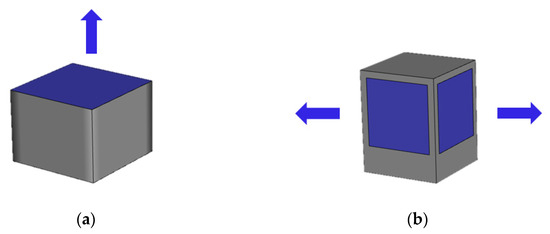
Figure 1.
Diagram of an upper vent: (a) vertical discharge pattern; (b) horizontal discharge pattern.
The fluid computational domains outside the upper vents were 200 m × 200 m × 100 m (length × width × height) (pollutant discharged vertically) and 400 m × 400 m × 50 m (length × width × height) (pollutant discharged horizontally). A hexahedral grid was used to subdivide the whole computational domain. To accurately simulate the jet effect of the air flow at the upper vents and to ensure computational efficiency, accuracy, and reliability, smaller grids were put around the upper vents, while larger girds were placed at the outer edge of the fluid computational space. Thus, the grids radiated from the upper vents and gradually became sparse. Figure 2 shows the partial profile of the grid around the upper vents for the two patterns of pollutant discharge. The total grid number was about 1.21 × 10⁶ for vertical pollutant discharge and 1.47 × 10⁶ for horizontal pollutant discharge.
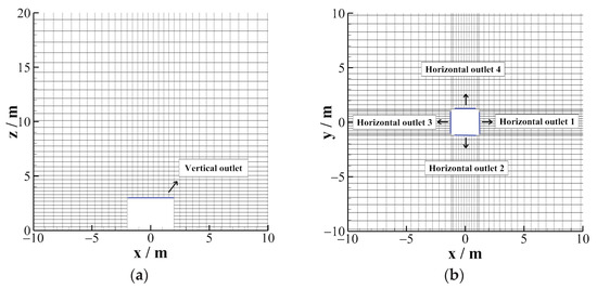
Figure 2.
Grid diagram of the upper vent: (a) vertical discharge pattern; (b) horizontal discharge pattern.
Figure 3a shows the velocity profile at a vertical height of 10 m from the ground, using different grid mesh numbers: 0.09 × 10⁶, 0.45 × 10⁶, 1.21 × 10⁶, and 2.80 × 10⁶. Figure 3b shows the velocity profile at a transverse distance of 10 m from the horizontal outlet, using different grid mesh numbers: 0.11 × 10⁶, 0.52 × 10⁶, 1.47 × 10⁶, and 3.00 × 10⁶. This indicates that the velocity distribution is not influenced by the increasing mesh number of the grids after it reaches 1.21 × 10⁶ for the outlets of vertically discharged pollutants and 1.47 × 10⁶ for the outlets of horizontally discharged pollutants. It is concluded that the grid independence requirement was met when the grid number reaches this approximate value.
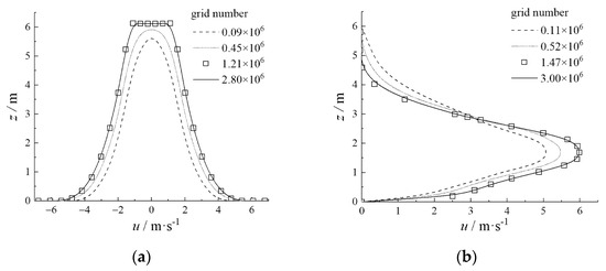
Figure 3.
Velocity profile of pollutant dispersion with different mesh numbers: (a) vertical discharge pattern; (b) horizontal discharge pattern.
2.3. Boundary Conditions
The non-slip and impenetrable boundary conditions (walls) were set for the walls of the upper vents and tunnel roofs. The Reynolds number in the near-wall region was quite low, and the standard wall function method was used to estimate the velocity distribution near the wall. The first grid node needed to be placed in the area where the laws of logarithm worked, thus ensuring that the dimensionless wall distance y+ fell between 30 and 300. For this study, y+ was guaranteed to be between 53 and 153 in all calculation conditions when the thickness of the first layer of the grid was 0.02102 m.
The Dirichlet boundary condition was set for the pollutant discharge outlet of the upper vents. The pollutant discharge velocity and concentration were provided according to the actual tunnel ventilation and possible working conditions in the stage of engineering operation. Due to the general characteristics of pollutant emission at fixed points and fixed volume in urban tunnels, and based on the sewage discharge parameters of Zijingang Tunnel’s upper vents in Hangzhou, this paper set the fixed discharge capacity (M = 40 mg/s) of the upper vents to study the rules of pollutant dispersion when the discharge velocity (V0) was 3 m/s, 4 m/s, 5 m/s, and 6 m/s. The discharge concentrations (C0) were then 0.83 mg/m3, 0.63 mg/m3, 0.5 mg/m3, and 0.42 mg/m3 at the corresponding discharge rates.
The Neumann boundary condition and pressure outlet were adopted for the boundary of the external air area in the computational region without considering the ambient wind. Taking the condition of ambient wind into consideration, the inlet of the external air area in the computational region was set as the Dirichlet boundary condition. The ambient wind speed was provided according to meteorological conditions, and the outlet of the external air area was set as Neumann boundary condition. It is thought that the normal gradient of the physical quantity is zero. The specific boundary conditions are shown in Figure 4.
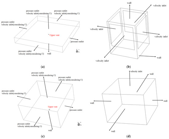
Figure 4.
Schematic diagram of the boundary conditions: (a) external air area for the horizontal upper vent; (b) upper vent in the horizontal discharge pattern; (c) external air area for the vertical upper vent; (d) upper vent in the vertical discharge pattern.
The ambient wind speed (U) at any elevation can be obtained by the following equation [25]:
U10 indicates the wind speed at 10 m elevation above ground, namely, the surface wind speed by the meteorological circle. The pollutant dispersion was computed when U10 was 0 m/s, 1 m/s, 2 m/s, 3 m/s, and 4 m/s. The ambient wind direction is the positive direction of the x-axis; p refers to the coefficient of roughness, which is related to landform and architecture environment. The wider and smoother a land is, the smaller p is. This study refers to the theses by Jiang et al. [26], where the α = 0.287 in the laboratory. The exponential distribution of wind speeds in the vertical direction can be achieved in Ansys Fluent 2019 R3 [27] by preparing the user-defined function (UDF).
3. Scale Model Test
The mathematical model was verified by the experimental results obtained with a 1/20 scale ventilation model tunnel with one upper vent from Zhejiang University. The schematic diagram of the model is shown in Figure 4. The length of the tunnel was 22 m, and the section size was 0.6775 m × 0.35 m. There are two types of upper vents, namely, a horizontal vent discharging pollutants and a vertical vent discharging pollutants, which can be replaced and spliced according to the test requirements. The discharge area of the vertical outlet was 0.2 m×0.2 m, and the area of the horizontal outlet was 0.1 m × 0.1 m (four sides). In the model tunnel, the airflow entered into a region of quadratic resistance law [28] when the tunnel wind speed was greater than or equal to 2.5 m/s.
In environmental impact analysis, NO2 is often used as a primary indicator. However, because of the toxicity of NO2, in this experiment we replaced NO2 with CO2, which is less harmful, cheaper, easy to obtain, and easy to measure. The pollutant-releasing device of the model test included a CO2 cylinder, a CO2 two-stage pressure-reducing valve (better pressure-stabilizing effect), and a vortex flow meter (DN200, CERTEON, China, Shanghai), as shown in Figure 5a.
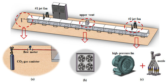
Figure 5.
Schematic diagram of the scale model: (a) pollutant release device; (b) axial fan; (c) jet fan simulator.
A stepless frequency conversion pipe fan was used to simulate axial flow fans (Figure 5b). A high-pressure variable-frequency fan was connected to the nozzle through a conductive pipe to simulate the jet fan (Figure 5c). The frequency converter was controlled by PLC 200 to start, stop, and regulate the speed of these model fans. The maximum fan volume in this model is 800 m3/h, and the maximum jet speed is 50 m/s. There are 2 jet fans and 1 set of top exhaust axial fans arranged in the model, as shown in Figure 5.
Figure 6a shows the distribution of wind speed and the CO2 concentration measurement points in the experimental model. In the experiment of pollutant diffusion from the vertical discharge outlet, a horizontal concentration sampling line was arranged at a height of 0.5 m from the ground, with a spacing of 0.05 m between the sampling points, for a total of 12 sampling points. When conducting the pollutant diffusion experiment at the horizontal discharge outlet, a horizontal concentration sampling line was arranged 0.09 m away from the ground, with a spacing of 0.3 m between the sampling points, using 10 sampling points in total, as shown in Figure 6b. Figure 6c shows the distribution of the wind speed measuring points on tunnel cross sections 1-1 and 2-2.
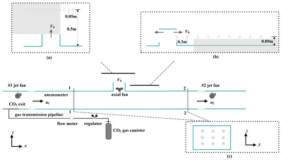
Figure 6.
Diagram of wind speed and concentration measurement points: (a) a series of CO2 concentration sampling points for the vertical outlet; (b) a series of CO2 concentration sampling points for the horizontal outlet; (c) wind speed measuring points for cross sections 1-1 and 2-2.
During the test, there was no ambient wind outside the model tunnel. The test process involved several steps: (1) the jet fans number 1 and 2 were turned on to ensure the air flow into a region of quadratic resistance law, and various values of V0 were obtained by regulating the speed of the axial-flow fan. Then, we waited a few minutes to make sure the airflow speed in the tunnel was stable; (2) in the tunnel, CO2 was released 10 m away from the upper vent to ensure that it was evenly mixed at the upper vent, and various values of discharge concentrations were obtained by changing the CO2 releasing flow; (3) the Testo 425 thermal anemometer (Testo AG, Baden-Wurttemberg, Germany) with accuracy of ±(0.03 m/s ± 5% reading) was used to collect 2 min speed data at each measuring point, and the average value of the 2 min data was taken as the speed of the measuring point. All the anemometers had been calibrated before the test; (4) the contaminated gas was sampled by the Scanivalve system, and the sample concentration was analyzed by high-resolution gas chromatograph. Samples of contaminated gas were collected via plastic tubes, which had an inside diameter of 1.6 mm. Ten samples were collected within 3 min at each sampling point, and the concentration of these samples was averaged as the concentration value of the sampling point. Each sampling point and Scanivalve scanning valve corresponding channel, Scanivalve outlet, and gas chromatograph sampling port were connected through a PVC pipe. In addition, an air pump was installed between the Scanivalve outlet and the gas chromatograph sampling port to speed up the sampling process. The tests were repeated twice to reduce random uncertainty. The coefficient of variation for most cases (more than 95%) was less than 5%, indicating that the measurement data only fluctuated in a small range, and the test results were reliable.
The average wind speed of tunnel Section 1-1 (u1) and 2-2 (u2) could be obtained by averaging the values measured at all measuring points on each section. The discharge wind speed of the upper vent V0 was calculated as V0 = (u1 − u2) S/F, where F is the total area of the discharge outlet, and S is the area of the tunnel cross section.
The variation curves of concentration C on the sampling line outside the vertical and horizontal discharge outlets with respect to x at different discharge velocities V0 were drawn. A numerical model was established under the same experimental conditions for the simulation. The comparison between the results of scale test and numerical simulation is shown in Figure 7. The CFD simulation results are consistent with the change trend of the test data, and the maximum error was 6.5%. The mathematical model demonstrated high accuracy and reliability.
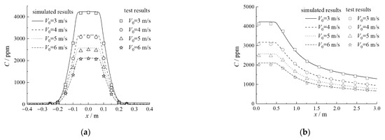
Figure 7.
Comparison between the results of numerical simulation and experimental model: (a) vertical discharge pattern; (b) horizontal discharge pattern.
4. Numerical Simulation Results and Discussions
4.1. Characteristics of the Air Flow in the Vertical Pollution Discharge Pattern
When the pollutants were discharged vertically from the upper vents, the flow structure and velocity vector with ambient wind were not considered, and the discharge velocity was V0 = 6 m/s, as shown in Figure 8, Figure 9 and Figure 10, displaying the flow structure and NO2 concentration distribution of the section with y = 0 m and z = 10 m at a discharge velocity of V0 = 6 m/s when the ambient wind speed was U = 1 m/s, 2 m/s, 3 m/s, and 4 m/s. Figure 11 presents the attenuation along the height direction (z-axis) of the dimensionless axial velocity Vmax/V0 of the jet under various working conditions.
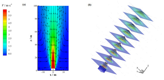
Figure 8.
(a) Flow structure and (b) velocity vector of the vertical outlet when V0 = 6 m/s without considering the ambient wind.
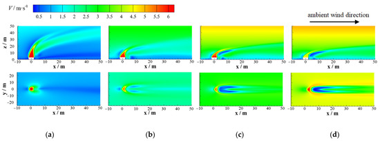
Figure 9.
Velocity profiles of the vertical outlet when V0 = 6 m/s without considering the ambient wind: (a) U = 1 m/s; (b) U = 2 m/s; (c) U = 3 m/s; (d) U = 4 m/s.
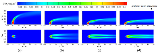
Figure 10.
NO2 distributions of the vertical outlet when V0 = 6 m/s without considering the ambient wind: (a) U = 1 m/s; (b) U = 2 m/s; (c) U = 3 m/s; (d) U = 4 m/s.
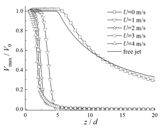
Figure 11.
Vmax/V0 attenuation of the vertical discharge jet under different U.
As seen in Figure 8, without ambient wind, the turbulent jet discharged from the vertical outlet continuously exchanged mass and momentum with the surrounding ambient air under transverse pulsation, driving the surrounding air flow so that the mass flow and cross-sectional area of the jet continuously increased along the height direction, forming a pyramidal flow field diffusing around. The dimensionless axial velocity Vmax/V0 attenuation of the jet was almost consistent with that of the free turbulent jet (Figure 11).
With ambient wind (Figure 9 and Figure 10), the polluted gas discharged from the vertical outlet diffused downwind and rose continuously under the combined action of its own kinetic energy through buoyancy effects caused by concentration difference and ambient wind. After a certain distance, it tended to be horizontal. This horizontal and vertical diffusion is called tail swinging and lifting of polluted air flow. The higher the ambient wind speed U, the faster the axial velocity attenuation of the jet due to the shear force of the transverse air flow (Figure 11), the greater the transverse diffusion of the polluted air flow in the horizontal direction, and the more significant the tail swing effect. In addition, because of the acceleration of the wind, the buoyancy and longitudinal diffusion of the exhaust gas were reduced, and the lifting effect of the exhaust gas was inhibited.
Therefore, the phenomenon of vertical pollutants discharging at the upper vent can be regarded as free buoyant jet diffusion under the momentum of ambient wind. Moreover, the movement of pollutants in the horizontal direction was mainly affected by the diffusion induced by the concentration difference and the convection caused by ambient wind.
4.2. Characteristics of the Air Flow in the Horizontal Pollution Discharge Pattern
Figure 12 displays the flow structure and velocity vector with discharge velocity of V0 = 6 m/s without considering the ambient wind when pollutants were discharged horizontally at the upper vents. Without ambient wind, the upper side of the turbulent jet discharged from the horizontal outlet was not limited, and the jet boundary expanded continuously under transverse pulsation. The lower side of the jet was close to the ground (distance from the ground, 0.8 m). Due to the Coanda effect [29], the jet could not entrain air, the static pressure of the gas was low, and the static pressure of the upper air flow of the jet was high. The difference in upper and lower pressure led to jet bending and a gradual close of the jet axis to the wall surface, forming a wall boundary layer.
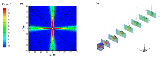
Figure 12.
(a) Flow structure and (b) velocity vector of the horizontal outlet when V0 = 6 m/s without considering the ambient wind.
Figure 13 presents the attenuation of the dimensionless axial velocity Vmax/V0 of the jet discharged from each outlet without considering the ambient wind. Near the horizontal outlet, Vmax/V0 decayed more slowly than that of a free jet, but faster than that of a three-dimensional wall jet. However, with the increase in the distance from the horizontal outlet, the attenuation rate of Vmax/V0 was gradually consistent with that of a three-dimensional wall jet.
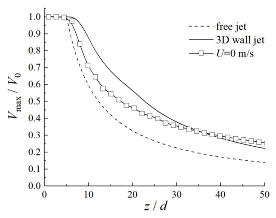
Figure 13.
Vmax/V0 attenuation of the horizontal discharge jet without considering the ambient wind.
Figure 14 and Figure 15 show the flow structure and NO2 concentration distribution in ambient wind direction corresponding to positive x-direction and discharge velocity V0 = 6 m/s for ambient wind speeds U = 1 m/s, 2 m/s, 3 m/s, and 4 m/s. Figure 16 presents the attenuation of the dimensionless axial velocity Vmax/V0 of the jet discharged from each outlet by considering the ambient wind.
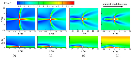
Figure 14.
Velocity profiles of the horizontal outlet when V0 = 6 m/s without considering the ambient wind: (a) U = 1 m/s; (b) U = 2 m/s; (c) U = 3 m/s; (d) U = 4 m/s.
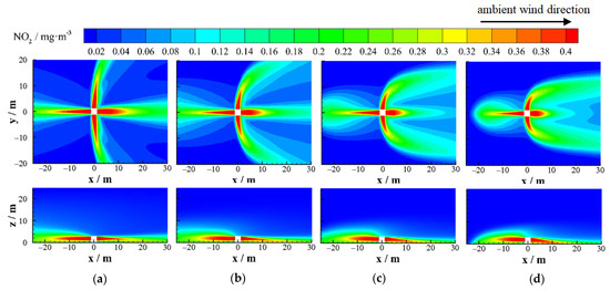
Figure 15.
NO2 distributions of the horizontal outlet when V0 = 6 m/s without considering the ambient wind: (a) U = 1 m/s; (b) U = 2 m/s; (c) U = 3 m/s; (d) U = 4 m/s.
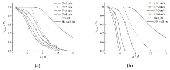
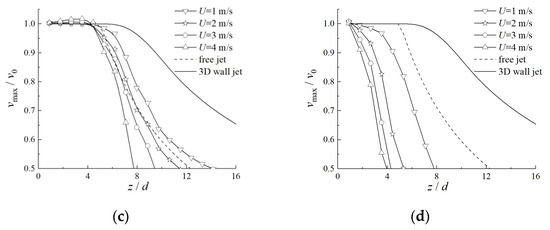
Figure 16.
Axial velocity attenuation of the horizontal discharge jet under different U: (a) horizontal outlet 1; (b) horizontal outlet 2; (c) horizontal outlet 3; (d) horizontal outlet 4.
Under the ambient wind, the polluted gas discharged from the horizontal outlet diffused in the downwind direction and upwards under the combined action of its own kinetic energy, through buoyancy effects caused by concentration difference and ambient wind. Compared with the case without ambient wind, a high-speed ambient wind could strengthen the turbulent mixing of polluted air flow and surrounding air, so that the core velocity of the jet at each outlet decayed faster, and the jet length was shorter, as shown in Figure 16.
Therefore, the phenomenon of pollutants discharging horizontally at the upper vent can be regarded as semi-confined buoyant jet diffusion under the momentum of the ambient wind. Moreover, the movement of pollutants in the horizontal direction was comprehensively affected by diffusion induced by concentration difference, jet momentum, and convection caused by the ambient wind.
4.3. Variation of the Environmental Impact Radius with Ambient Wind Velocity
Let r be the horizontal distance from the center of the upper vent. Then, Cmax is set as the maximum concentration of pollutants on the cylinder, with the center of the upper vent as the origin at the radius r. Cmax of the horizontal outlet when the discharge velocity V0 is 6 m/s and the ambient wind U is 0 m/s is presented in Figure 17.
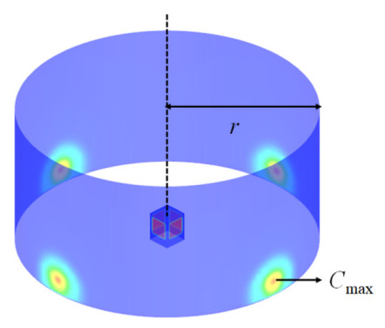
Figure 17.
Cmax diagram.
The concentration limits of various pollutants in various ambient air function zones are indicated in “Ambient Air Quality Standards” (GB3095-2012) issued by the Chinese government. Based on this, 0.2 mg/m3, i.e., the NO2 hourly average concentration limit of the class II ambient air function zone, was adopted in this study as the environmental standard. Meanwhile, the distance at which the concentration of pollutants discharged from the upper vent decreased to 0.2 mg/m3 was deemed as the environmental impact radius rcriti of the upper vent. Since the value of rcriti has a certain impact on both the planning layout of buildings around the tunnel and the valuation of the surrounding land, it is necessary to study the rcriti value of NO2 emission. The rcriti of the vertical outlet when the wind velocity V0 was 6 m/s and the ambient wind U was 3 m/s is shown in Figure 18.
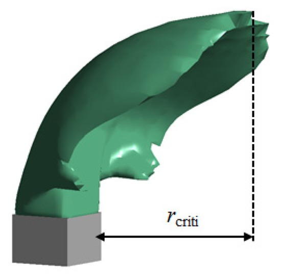
Figure 18.
Diagram of rcriti.
The distribution of Cmax of the vertical and horizontal outlets along the r direction under various ambient wind velocities U, when the discharge velocity of the vent V0 was 6 m/s, is shown in Figure 19. Figure 20 shows the environmental impact radius rcriti of pollutants discharged from the vertical and horizontal outlets under different ambient wind speeds U when the discharge velocity V0 was 3 m/s, 4 m/s, 5 m/s, and 6 m/s.
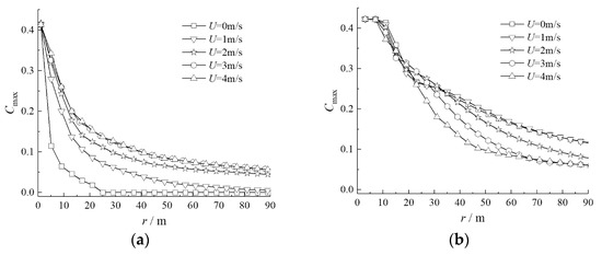
Figure 19.
Attenuation of Cmax along the r direction for various U: (a) vertical discharge pattern; (b) horizontal discharge pattern.
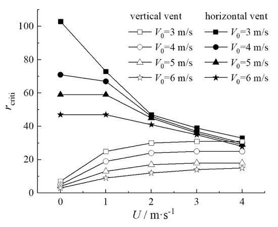
Figure 20.
Variation of rcriti with U under for V0.
As can be observed from Figure 19a, Cmax gradually attenuated with the rising of r under various U for the vertical outlet. In particular, Cmax near the upper vent decreased at a faster velocity, whereas Cmax far from the upper vent diminished slowly. Moreover, for U ≤ 3 m/s, the larger U was, the greater the shear force of the lateral airflow suffered by the polluted airflow, the greater the horizontal diffusion, and the more significant the tail swing effect obtained in combination with the flow structure shown in Figure 9 and Figure 10. Hence, the slower the attenuation in Cmax, the larger the rcriti (as shown in Figure 20). When U = 1 m/s, for instance, rcriti was 9 m; when U =3 m/s, rcriti wase 14 m, up by 56%. The attenuation rate of Cmax under various U values started to converge when U ≥ 3m/s. At the same time, rcriti also tended to be invariant according to Figure 20.
As can be seen from Figure 19b, Cmax first remained unchanged with the rising of r under various U for the horizontal outlet, and then began to decrease when far from the upper vent (r was roughly greater than 10 m). In addition, Cmax under various U tended to converge at the scope approaching the upper vent. By contrast, U had a significant impact on the attenuation rate of Cmax at the scope far from the upper vent (r was roughly greater than 20 m), that is, the greater the U value, the better the contribution to the turbulent mix of pollution gas and ambient air. Together with the flow structure shown in Figure 14 and Figure 15, the shorter the discharge jet length of each outlet, the faster the decrease of Cmax, resulting in the smaller rcriti (as shown in Figure 20). To be specific, when U = 1 m/s, rcriti was 47 m; when U = 4 m/s, rcriti was 28 m, reduced by 40%.
Further, rcriti decreased with the rising of V0 under various U for the vertical outlet, according to Figure 20. When there was ambient wind, V0 was more sensitive to the impact of rcriti than without ambient wind. To be clear, when V0 increased from 3 m/s to 6 m/s, in the case of no ambient wind, rcriti declined to 3 m from 7 m, with a reduction of 4 m. By contrast, rcriti was reduced to 15 m from 31 m when there was ambient wind, showing a reduction up to 15 m.
Regarding the horizontal outlet, rcriti also decreased with the increase of V0 under various U for the horizontal outlet. The greater the ambient wind U, the weaker the impact of V0 on rcriti. After U, a rcriti, however, merely decreased with the increase of U, rather than varying with the changing V0.
Further, the rcriti of the vertical outlet was smaller than that of the horizontal outlet within the parameter range when V0 and U were constant, in this study. However, a smaller variation was found in rcriti of the upper vents for the two discharge patterns when V0 was smaller and U was larger. When V0 = 3 m/s and U = 4 m/s, for instance, the environmental impact radius rcriti of the vertical and horizontal outlets were approximately equal, being 31 m and 33 m, respectively.
5. Conclusions
Several conclusions can be drawn from this study:
- (1)
- The pollutant emission of the upper vent under a vertical discharge pattern can be considered as the free buoyant jet diffusion under the impact of the momentum of ambient wind. The maximum concentration of pollutants Cmax gradually decreased with the increase in the horizontal distance r from the upper vent under varied ambient wind velocities U. The environmental impact radius rcriti of the pollutant increased with the increase of U when U ≤ 3 m/s, and was free from the impact of U after U > 3 m/s.
- (2)
- The emission under the horizontal discharge pattern can be regarded as the semi-confined buoyant jet diffusion under the impact of the momentum of ambient wind. Cmax first remained unchanged with the rising of the horizontal distance r from the upper vent under various U, and then gradually decreased. The attenuation rate of Cmax was nearly independent of the impact of U in the range approaching the upper vent. However, when it was far from the upper vent, the greater the value of U, the faster the attenuation of Cmax, and the smaller the environmental impact radius rcriti.
- (3)
- When the discharge capacity was constant, the environmental impact radius of the upper vent under both vertical and horizontal discharge patterns decreased with the increase of the discharge velocity V0. When there was ambient wind, V0 was more sensitive to the impact of rcriti for the vertical outlet, whereas V0 was more sensitive to the impact of rcriti for the horizontal outlet when there was no ambient wind. Moreover, the environmental impact radius, rcriti, of the vertical outlet was smaller than that of the horizontal outlet for the range of parameters considered.
- (4)
- It is worth noting that the upper vent featuring “emission in high concentration and low wind velocity” can improve more significantly the environmental air quality inside a longitudinal ventilation tunnel when the total air volume and discharge capacity are constant. In this regard, the annual environment wind velocity of the tunnel and the impact of the upper vent on the environment inside and outside the tunnel should be considered before designing top vents for tunnels.
Author Contributions
Conceptualization and Writing, X.Z.; Funding acquisition, X.Z. and K.W.; Supervision, K.Z.; Validation, X.Z. and K.Z.; Writing—Original Draft Preparation, X.Z.; Writing—Review and Editing, K.W. and K.Z. All authors have read and agreed to the published version of the manuscript.
Funding
This research was funded by the Natural Science Basic Research Program of Shaanxi (Program No.2020JQ-779), Shaanxi Provincial Education Department (Program No. 20JK0840), Ningbo Transportation Science and Technology Plan Project (202113) and the Natural Science Foundation of Zhejiang province (No. LY19E080028).
Institutional Review Board Statement
We choose to exclude this statement because this study did not involve humans or animals.
Informed Consent Statement
We choose to exclude this statement because this study did not involve humans.
Data Availability Statement
We choose to exclude this statement because this study did not report any data.
Conflicts of Interest
The authors declare no conflict of interest.
References
- Du, T.; Yang, D.; Peng, S.N.; Xiao, Y.M. A method for design of smoke control of urban traffic link tunnel (UTLT) using longitudinal ventilation. Tunn. Undergr. Space Technol. 2015, 48, 35–42. [Google Scholar] [CrossRef]
- Gong, C.J.; Ding, W.Q.; Soga, K.; Mosalam, K.M. Failure mechanism of joint waterproofing in precast segmental tunnel linings. Tunn. Undergr. Space Technol. 2019, 84, 334–352. [Google Scholar] [CrossRef]
- Wang, M.N.; Wang, X.; Yu, L.; Deng, T. Field measurements of the environmental parameter and pollutant dispersion in urban undersea road tunnel. Build. Environ. 2019, 149, 100–108. [Google Scholar] [CrossRef]
- Zhang, H.H.; Hou, Y.G.; Wu, K.J.; Zhang, T.H.; Wu, K.; Zhang, X. Study on Mechanism of Series-Flow of Pollutants between Consecutive Tunnels by Numerical Simulation. Appl. Sci. 2019, 9, 4125. [Google Scholar] [CrossRef] [Green Version]
- Zhang, X.; Zhang, T.H.; Zhu, K.; Huang, Z.Y.; Wu, K. Numerical Research on the Mixture Mechanism of Polluted and Fresh Air at the Staggered Tunnel Portals. Appl. Sci. 2018, 8, 1365. [Google Scholar] [CrossRef] [Green Version]
- Jin, S.K.; Jin, J.L.; Gong, Y.F. A theoretical explanation of natural ventilation at roof openings in urban road tunnels. Tunn. Undergr. Space Technol. 2020, 98, 103345. [Google Scholar] [CrossRef]
- Bari, S.; Naser, J. Simulation of airflow and pollution levels caused by severe traffic jam in a road tunnel. Tunn. Undergr. Space Technol. 2010, 25, 70–77. [Google Scholar] [CrossRef]
- Raaschou-Nielsen, O.; Andersen, Z.J.; Jensen, S.S.; Ketzel, M.; Sorensen, M.; Hansen, J.; Loft, S.; Tjonne, A.; Overvad, K. Traffic air pollution and mortality from cardiovascular disease and all causes: A Danish cohort study. Environ. Health 2012, 11, 60. [Google Scholar] [CrossRef] [PubMed] [Green Version]
- Hoek, G.; Krishnan, R.M.; Beelen, R.; Peters, A.; Ostro, B.; Brunekreef, B.; Kaufman, J.D. Long-term air pollution exposure and cardio-respiratory mortality. Environ. Health 2016, 12, 43. [Google Scholar] [CrossRef] [Green Version]
- Zhong, X.C.; Zeng, Z. Distribution of Harmful Gas Concentration in Highway Tunnel with Natural Ventilation. J. Railw. Eng. Soc. 2006, 9, 44–49. [Google Scholar]
- Huo, Z.Y.; Long, E.S.; Wang, J. Influence of Urban Highway Tunnel Upper Vents Groups Number on Natural Ventilation Efficiency. Lect. Notes Electr. Eng. 2014, 263, 357–363. [Google Scholar]
- Jin, S.K.; Jin, J.L.; Gong, Y.F. Natural ventilation of urban shallowly-buried road tunnels with roof openings. Tunn. Undergr. Space Technol. 2017, 63, 217–227. [Google Scholar] [CrossRef]
- Guo, Q.; Zhu, H.; Zhang, Y.; Shen, Y.; Zhang, Y.P.; Yan, Z.G. Smoke flow in full-scale urban road tunnel fires with large cross-sectional vertical shafts. Tunn. Undergr. Space Technol. 2020, 104, 103536. [Google Scholar] [CrossRef]
- Fan, C.G.; Chen, J.; Zhou, Y.; Li, L.J.; Zhang, J.Q.; Fan, M.H.; Liu, X.P. A simple method to improve smoke exhaust effectiveness of a shallow-buried urban tunnel fire with natural ventilation. Combust. Sci. Technol. 2021, 193, 355–378. [Google Scholar] [CrossRef]
- Fan, C.G.; Chen, J.; Mao, Z.L.; Zhou, Y.; Mao, S.H. A numerical study on the effects of naturally ventilated shaft and fire locations in urban tunnels. Fire Mater. 2019, 43, 949–960. [Google Scholar] [CrossRef]
- Yao, Y.Z.; Zhang, S.G.; Shi, L.; Cheng, X.D. Effects of shaft inclination angle on the capacity of smoke exhaust under tunnel fire. Indoor Built Environ. 2019, 28, 77–87. [Google Scholar] [CrossRef]
- Fan, C.G.; Ji, J.; Wang, W.; Sun, J.H. Effects of vertical shaft arrangement on natural ventilation performance during tunnel fires. Int. J. Heat Mass Transf. 2014, 73, 158–169. [Google Scholar] [CrossRef]
- Yu, J.; Tian, L.; Zhuang, W.; Yang, J. Prediction of the Pollutant Diffusion Discharged from Wind Tower of the City Traffic Tunnel. Tunn. Undergr. Space Technol. 2014, 42, 112–121. [Google Scholar] [CrossRef]
- Huang, Y.; Gong, X.; Peng, Y.; Lin, X.; Kim, C. Effects of the Ventilation Duct Arrangement and Duct Geometry on Ventilation Performance in a Subway Tunnel. Tunn. Undergr. Space Technol. 2011, 26, 725–733. [Google Scholar] [CrossRef]
- Launder, B.E.; Spalding, D.B. The numerical computation of turbulent flows. Int. J. Numer. Methods Fluids. 1974, 15, 127–146. [Google Scholar] [CrossRef]
- Stathopoulos, T. Computational Wind Engineering: Past Achievements and Future Challenges. J. Wind Eng. Ind. Aerodyn. 1997, 67–68, 509–532. [Google Scholar] [CrossRef]
- Rollet-Miet, P.; Laurence, D.; Ferziger, J. LES and RANS of Turbulent Flow in Tube Bundles. Int. J. Heat Fluid Flow 1999, 20, 241–254. [Google Scholar] [CrossRef] [Green Version]
- Yang, Y.R.; He, C.; Zeng, Y.H. Numerical simulation for the pollution effect between portals of twin highway tunnels. Mod. Tunn. Technol. 2009, 46, 94–98. [Google Scholar]
- Tabatabaian, M. CFD Module: Turbulent Flow Modeling; Mercury Learning & Information: Duxbury, MA, USA, 2015; p. 43. [Google Scholar]
- Lou, W.J.; Liang, H.C.; Li, Z.H.; Zhang, L.G.; Bian, R.; Zhang, S.W. Research on Wind Environment of Residential Districts in Hangzhou Based on Numerical Simulation. Acta Aerodyn. Sin. 2018, 36, 791–797. [Google Scholar]
- Jiang, W.M.; Yu, H.B.; Xie, G.L.; Wu, J.; Zhu, H.G.; Sun, H.N. An experiment study on environmental impact of automobile exhaust from urban transportation tunnels. ACTA Sci. Circumstantiae 1998, 18, 188–193. [Google Scholar]
- Wang, F.J. Computational Fluid Dynamics Analysis, 1st ed.; Tsinghua University Press: Beijing, China, 2004; pp. 21–22. [Google Scholar]
- Wang, Y.Q.; Xia, F.Y.; Xie, Y.L. Physical Model Experiment on Complementary Ventilation of Extra-long Highway Tunnel. China J. Highw. Transp. 2014, 27, 84–90. [Google Scholar]
- Panitz, T.; Wasan, D.T. Flow Attachment to Solid Surfaces: The Coanda Effect. AIChE J. 1972, 18, 51–57. [Google Scholar] [CrossRef]
Publisher’s Note: MDPI stays neutral with regard to jurisdictional claims in published maps and institutional affiliations. |
© 2021 by the authors. Licensee MDPI, Basel, Switzerland. This article is an open access article distributed under the terms and conditions of the Creative Commons Attribution (CC BY) license (https://creativecommons.org/licenses/by/4.0/).