Abstract
Magnetic field measurement is fundamental to nuclear magnetic resonance rotation sensors (NMRRS). A phase-locked loop (PLL)-based measurement with two nuclear isotopes is commonly applied to observe the magnetic field. However, the phase-loop and frequency-loop of the nuclear isotopes cannot be optimized simultaneously by a PLL-based method. In this paper, an approach based on a linear active disturbance rejection controller (LADRC) is proposed for synchronous phase-loop control of the two nuclear isotopes. Meanwhile, the frequencies of the nuclear isotopes are observed by linear extended state observers (LESOs). The phase and frequency loops can be decoupled and optimized with the proposed method. An experimental NMRRS prototype used for verification is built. The effectiveness and the feasibility of the proposed method are validated with the experimental results.
1. Introduction
In recent years, extensive research on quantum theory has resulted in the rapid development of atomic sensors. Atomic rotation sensors with ultra-high sensitivity and a small volume are positive prospects for modern inertial navigation systems (INS) [1,2,3]. Among the atomic spin rotation sensors, the nuclear magnetic resonance rotation sensor (NMRRS), which is featured as low cost, small volume, high precision, and insensitive to external vibrations, is recognized as one of the promising candidates for the next generation of rotation sensors [4,5,6].
NMRRS accomplishes rotation sensing by observing a shift in the Larmor frequency of nuclear spins in an applied magnetic field. Around the early 1960s, small-scale research and case studies on NMRRS began to emerge [7,8]. Over the next two decades, extensive research was carried out, aiming at providing an accurate, low-cost NMRRS, which is an alternative to the spinning-wheel rotation sensor in certain applications. However, the ring-laser gyroscope (RLG) [9] and fiber-optic gyroscope (FOG) [10], utilizing the Sagnac effect, have rapidly developed to be the leading contender of rotation sensors. The research of NMRRS hwas suspended before its potential was fully realized due to being incapable of providing considerable advantages. However, the research of NMRRS has been revived in the 20th century due to the success of the atomic clock and magnetometer [11,12]. Lots of former issues can be reconsidered using new concepts.
A considerable amount of literature has described the role of magnetic-field measurement [13,14,15,16]. According to [13], a 1°/h bias corresponds to a magnetic field error of 100 fT given the gyromagnetic ratio for 129Xe of 2π∙10 MHz/T. In the earliest proposals for NMRRS, the magnetic field could not be measured, which results in a severe limitation on accuracy by uncertainties in the magnitude of the magnetic field. By introducing a second set of resonant nuclei isotopes, the literature [17] makes it possible to measure the magnetic field. A variant with four frequencies available for measurement is mentioned in [18]; however, it is not commonly applied due to the stringent requirement for the two steady, equal, and opposite magnetic fluxes. Thus, the two-isotope (129Xe and 131Xe) solution of magnetic field measurement is mainly considered in this paper.
Traditionally, the observed precessional rate is assumed to be equal to the resonance frequency in previous research. These assumptions ignored the transient process of the observer. To make an expected differential rotation measurement, the transient processes of two nuclear isotopes need be synchronous, which is determined by the synchronous performance of the phase-locked loop (PLL). Moreover, observing the frequencies of the two isotopes makes it possible to measure the applied magnetic field. A monotone decreasing step response of the observed frequency can simplify the design of the feedback controller of the magnetic field. Both phase and frequency loops are determined by the parameters of the controllers. It turns out to be a tradeoff, which means that the performance of both loops cannot be optimized at the same time.
A LADRC is a robust, model-independent approach developed from the classic PID control strategy [19,20]. One of the most significant features of a LADRC is the linear extended state observer (LESO), which is designed to observe the unknown disturbance without establishing an accurate plant model. In [21,22,23], a linear ESO is used to enhance control dynamics of the PLL of the power system, which finds us a new way to overcome the weakness of the traditional method that appears in the NMRRS.
Therefore, this study makes a major contribution to research on magnetic field measurement by demonstrating a LADRC-based method. The two nuclear spin oscillators are driven synchronously by the LADRC. Two LESOs are designed to observe the Larmor precessional rate of both isotopes. The manipulations of the phase and frequency loops are decoupled, and the optimized performance can be achieved by proper parameter tuning.
The rest of this paper is organized as follows. The conventional magnetic-field measurement method based on the PLL is briefly introduced in Section 2. Meanwhile, the introduction of the experimental NMRRS and the magnetic field measurement errors are analyzed in this section. Section 3 is concerned with the methodology used for this study. Finally, the experimental setup is introduced in Section 4, and the experimental results are illustrated in Section 5. The main conclusions are drawn in Section 6.
2. Dual Nuclear Magnetic-Field Measurement Method
2.1. PLL-Based Dual Nuclear Magnetic-Field Measurement Method
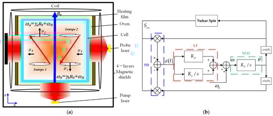
Figure 1a shows a typical experimental arrangement of the NMRRS. A vapor temperature-controlled glass cell is mounted in the NMRRS. The vapor cell contains two noble gas nuclei (129Xe and 131Xe), an alkali–metal atom(87Rb), and buff gas. A circularly polarized pumping beam, whose wavelength is equal to the D1 line of the Rb atoms, orients parallel to an applied magnetic field B0. Thereby, the valence electrons of the alkali metal are spin-polarized. The collisions between the alkali-metal atoms and noble gas atoms transfer some of the electron-spin polarization to the nuclei of the noble gas, which produced the coherency of the nuclear spin.
Figure 1.
Typical schematic diagram of the NMRRS. (a) is the typical experimental arrangement of the NMRRS. (b) is the PLL-based single nuclear feedback control.
The nuclear spins are made to precess about B0 by the oscillating magnetic field B+ Xe applied along the x-axis, producing a net nuclear magnetization. The linear polarized probe light to read out the spin precession is detected by a balanced detector after passing through the vapor cell. The signal is demodulated in a lock-in amplifier to obtain the two nuclear spins. The frequency of the nuclear spin precession can be observed by PLL circuits. When the sensor is rotating about the axis of the applied field B0 at a frequency ωr, the measured Larmor precession frequency is
where is the gyromagnetic ratio of the nucleus.
Figure 1b shows a conventional block diagram of the PLL-controlled nuclear spin. The PLL controls the coherent spin resonance with the oscillating magnetic field and observes the Larmor frequency of the nuclear spin.
From Equation (1), it is not possible to distinguish between changes in caused by fluctuations in B0 from changes solely due to rotation. It will be necessary for any practical version of the NMRRS to maintain the magnitude of B0 precisely or, alternatively, to employ techniques that effectively compensate for any variations in the value of caused by B0 fluctuation.
As shown in Figure 1, two isotopes precessing in Larmor frequency ( and ) are introduced to determine the rotation rate. The rotation rate is independent of the magnetic field B0.
2.2. Dynamic Model of the PLL Controlled Spin
The dynamics of the noble gas spin ensemble is the basis of this method. The motion of the magnetization vector of the Xe nuclei is described by Bloch equations as follows:
where , and are the three components of the magnetization vector. Bx, By, and Bz are the magnetic field. T1 and T2 are the longitudinal and transverse relaxation times of noble gas. γ is the gyromagnetic ratio. is the relaxation ratio.
For convenience, a phasor representation of , is defined as,
Meanwhile, Equation (4) could be rewritten as a phasor representation,
A main magnetic field is applied in the z-axis direction to make the nucleon ensemble precession, and a drive magnetic field B1 with the same precession frequency is added in the transverse x-axis. Thus, the evolution equation of the amplitude and phase of the spin magnetic moment of the nucleon can be obtained by introducing Equation (5) into Equation (6),
where and .
It can be seen from the above formula that the precession phase dynamics of the noble gas nucleon is a nonlinear process, and its changing rate is determined by the detuning phase and intensity of the driving magnetic field, the amplitude of the z-axis magnetic moment, and the amplitude of the transverse magnetic moment.
When the NMR gyro operates, the nuclear spin resonator is in resonance or near detuning state, and the changing rate of is very small, which could be ignored. Therefore, substituting into Equation (7), the following can be obtained,
Substituting Equation (6) into Equation (5), it can be derived,
Assuming , , a differential equation about the detune phase y could be obtained,
Considering the detuning phase y is extremely small, Equation (11) can be linearized as
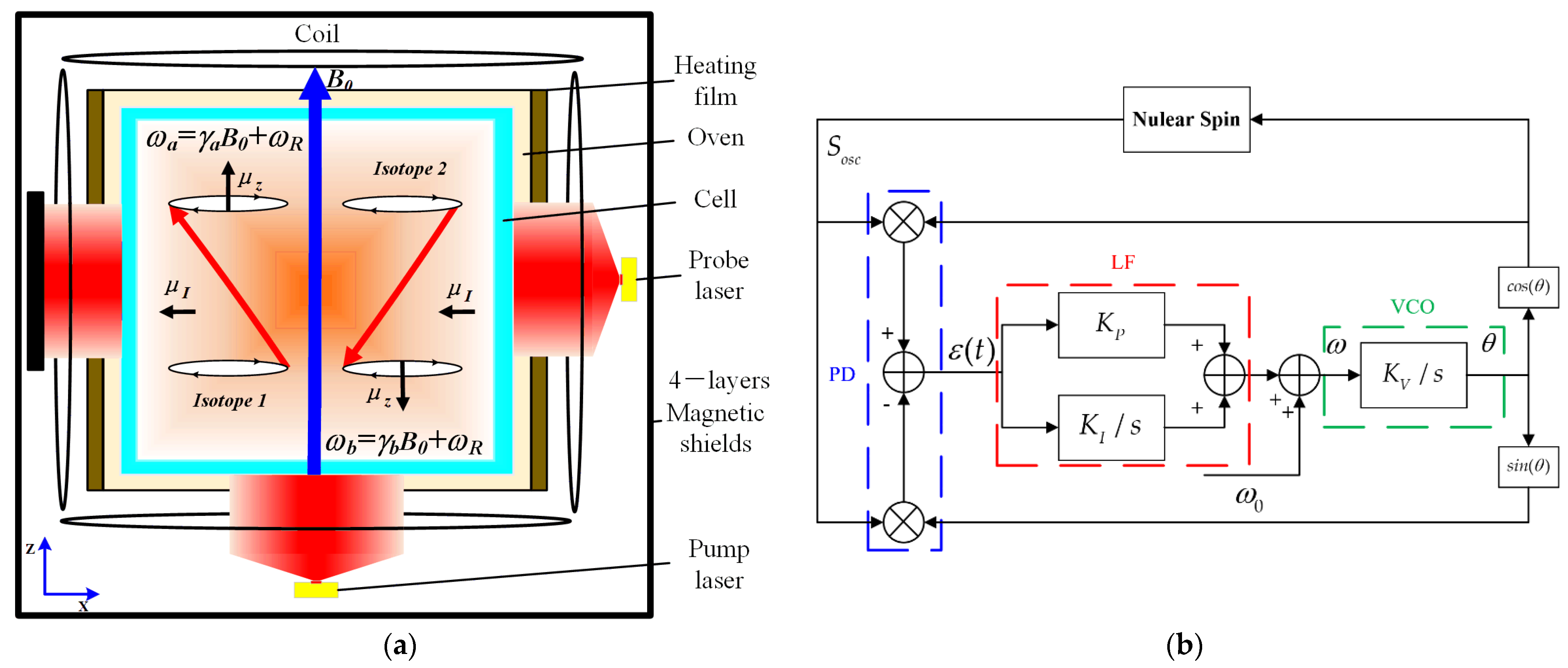
Thus, the block diagram of the PID-based nuclear spin control system is shown as Figure 2.
Figure 2.
Block diagram of PLL-based nuclear spin control loop.
D(s) is the external disturbance, Y(s) is the observed detuning phase, R(s) is the reference phase, and U(s) is the output of the controller. Gp(s) and Gc(s) is the transfer function of the plant and the controller, respectively.
According to Equation (12), Gp(s) can be obtained,
The loop filter used in this paper is PI controller, then
The close-loop transfer function of the system is
represents the phase tracking performance and represents the frequency observing performance of the system.
2.3. Analysis of Transient Errors in Magnetic Measurement
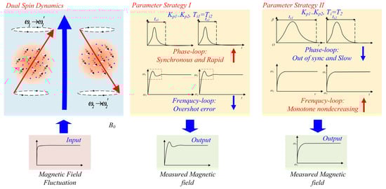
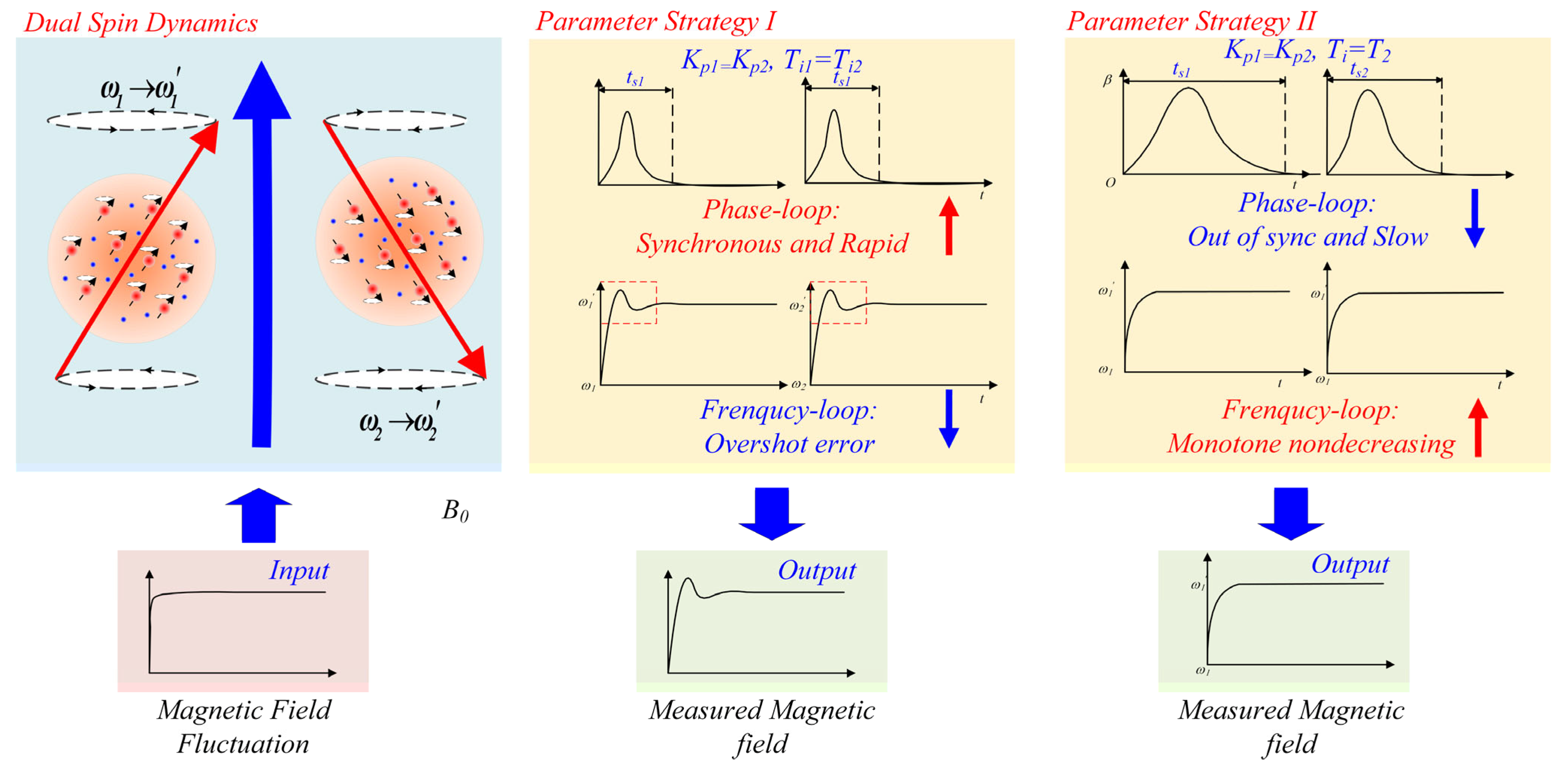
In this subsection, two strategies were proposed based on the PLL method. Analysis of the strengths and weaknesses of both strategies were given. As is shown in Figure 3, the two resonant nuclear oscillators with frequencies ( and ) are maintained by PLLs. The magnetic field fluctuation changes the Larmor frequencies of the nuclei, which makes the spin oscillators off-resonant. Under the control of PLL, the spin oscillators return to resonant in a new set of frequencies ( and ).
Figure 3.
Analysis of transient errors of the magnetic-field measurement.
In the applications of NMRRS, the tasks of the spin control are
- Synchronously tracking the detuned phase of the two isotopes, which makes the differential effect more efficient.
- Observing the Larmor frequency of the two isotopes with a monotone nondecreasing step-response. This will suppress errors of the magnetic field measurement and simplify the magnetic field control loop.
As they are in Equations (15) and (16), the parameters in the closed-loop transfer function are , and . In NMRRS, the bandwidth of the controller (determined by and ) is ten times greater than . Thus, the controller parameters play the dominant role in the synchronous transient processes. Two strategies were proposed here:
- (1)
- Strategy I
The controller parameters of the two spins can be set as equal to obtain a better synchronous performance of the phase loop.
, are the P gains, , are the integral time constants of the two isotope control loops, respectively.
Each of the two poles in (16) is greater than the zero (1/), which is necessary to achieve a fast response of the phase. Based on the theory in [24], an overshot inevitably appears in the step response.
- (2)
- Strategy II
The controller parameters of the two spins can be set to equal the lifetime of the nuclear spin to obtain a better observation of the frequency loop.
, are the transverse relaxation times of the two isotopes.
Then, the system in Equation (16) will be simplified as
It is obvious that monotone nondecreasing step response of the two spin frequency-loops can be achieved. However, the tracking response of the phase loop cannot be synchronous and fast due to the different lifetimes of the two isotopes.
Overall, based on the PLL method, it is a conflict to improve the phase loop or the frequency-loop performance at the same time. Both of the two strategies given above cannot achieve the goal solely.
3. LADRC-Based Synchronous Control Method
In this section, by employing the LADRC theory, a magnetic field measurement method is presented. The LADRC of each isotope is designed to control the spins synchronously. Meanwhile, the Larmor frequencies are observed by the LESOs without overshooting.
3.1. LADRC Design
On the basis of the preliminarily established phase dynamic model, we extended the fluctuation as an additional state variable, and the system state was extended to . Letting represent the extended state of , then the original plant in (13) can be rewritten as,
The task of the observer design is not only observing the unmeasured system states (i.e., x1) but also estimating the modeling uncertainty for controller compensation in real time. Let denote the estimate of x. The extended system model can be rewritten as
The error of the observer is defined as,
Thereby,
Assuming that the matrix (A-GC) is a Hurwitz matrix. The error of the observer e is converged to 0,
Denoting that
The characteristic equation of is
The poles are placed at ,
The gain matrix of the observer is obtained,
The LESO is formed as
As it is shown in Equation (29), the LESO always converges as . The total disturbance can be estimated by the LESO and the feedback control value is designed as
where Kc is the feedback gain and r is the refer input.
3.2. Analysis in Frequency Domain
By some deduction-based literature [24], the closed-loop transfer function of the phase loop and the frequency loop of LADRC are given by the expressions:
where
From the Routh stability criterion, systems in Equations (31) and (32) are always stable because .
According to the analysis in Section 2, a monotone nondecreasing step response without overshoot is required. Based on theorem in [24,25], a specific combination of control parameters is presented to have monotone nondecreasing step responses.
Corollary 1.
Let, and , then the system in Equation (32) has a monotone nondecreasing step response.
Proof of the corollary.
The precondition means that the absolute values of the three real poles are
Thus, Equation (32) can be decomposed as
The damping ratio of the system in Equation (35) is ; therefore, a monotone nondecreasing step response can be achieved. □
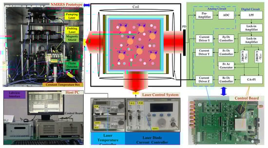
4. Experimental Setup
The overall NMR rotation sensor experimental setup is shown in Figure 4. The experimental setup consists of the NMR sensor prototype, the turntable, the laser control system, and the sensor control circuit. The NMR sensor prototype and the breadboard are mounted on the turntable. The laser control system (TED 200C and LDC 200C) is used to produce the pumping and probing laser beam. The laser beam is induced into the prototype by the optical fiber.
Figure 4.
Experimental setup of the NMRRS.
The comagnetometer signal (Spd) is collected by the photodetector. Then, the signal is sampled and converted to a digital signal by the pre-amplifier circuit. To process the digital signal and the electrical signal, the sensor control circuit using a digital signal processor (DSP, TMS 320F28335) and a field-programmable gate array (FPGA, Xilinx Kintex7 XC7K480T) has been implemented to control the magnetic field in the NMR rotation sensor.
As is shown in Figure 4, the signal is parametrically modulated at the alkali Larmor frequency (100 kHz range). The input signal is demodulated (32-bit CORDIC rotate algorithm) by a lock-in amplifier (LIA) to obtain the oscillation signal. By a low-pass filter, the oscillation signals of the Xe isotopes are separated and the phase of the oscillation signals are detected by the phase detector (32-bit CORDIC vector algorithm). The magnetic field estimation method based on the traditional PLL controller and the proposed synchronous estimation method based on LESO are implemented in the FPGA. The PLL or LADRC will keep the Xe isotopes resonant with the Larmor frequency by adjusting the frequency of the numerically controlled oscillator (NCO). Additionally, the estimation algorithms can obtain the magnitude of the magnetic field according to the frequencies of the NCO. The photograph of the experimental platform which consists of the control system and the experimental prototype is shown in Figure 4.
5. Experimental Evaluation
In this section, several experimental results are shown to validate the effectiveness of the proposed method in this paper. According to the analysis above, the proposed synchronous control method is designed to control the Xe isotopes synchronously, and the errors caused by the imbalance of the transient process can be reduced. For this reason, in this section, the synchronous control performance and the measurement performance were tested and evaluated first by comparison to the traditional PLL-based method. The influences of the adjustable parameters were tested, and a detailed parameter tuning method of the proposed controller was given.
5.1. Transient Response Performance Comparison
In this experiment, the effectiveness of the proposed method was examined. A step signal (5 nT) was added to the magnetic field of z-axis. The responses of the PLL-based method (parameter strategy I and II) and the LADRC-based method were recorded to be a comparative experiment. The parameters of the controller are listed in Table 1.
Table 1.
Parameters of the Tested Method.
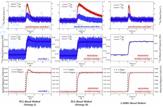
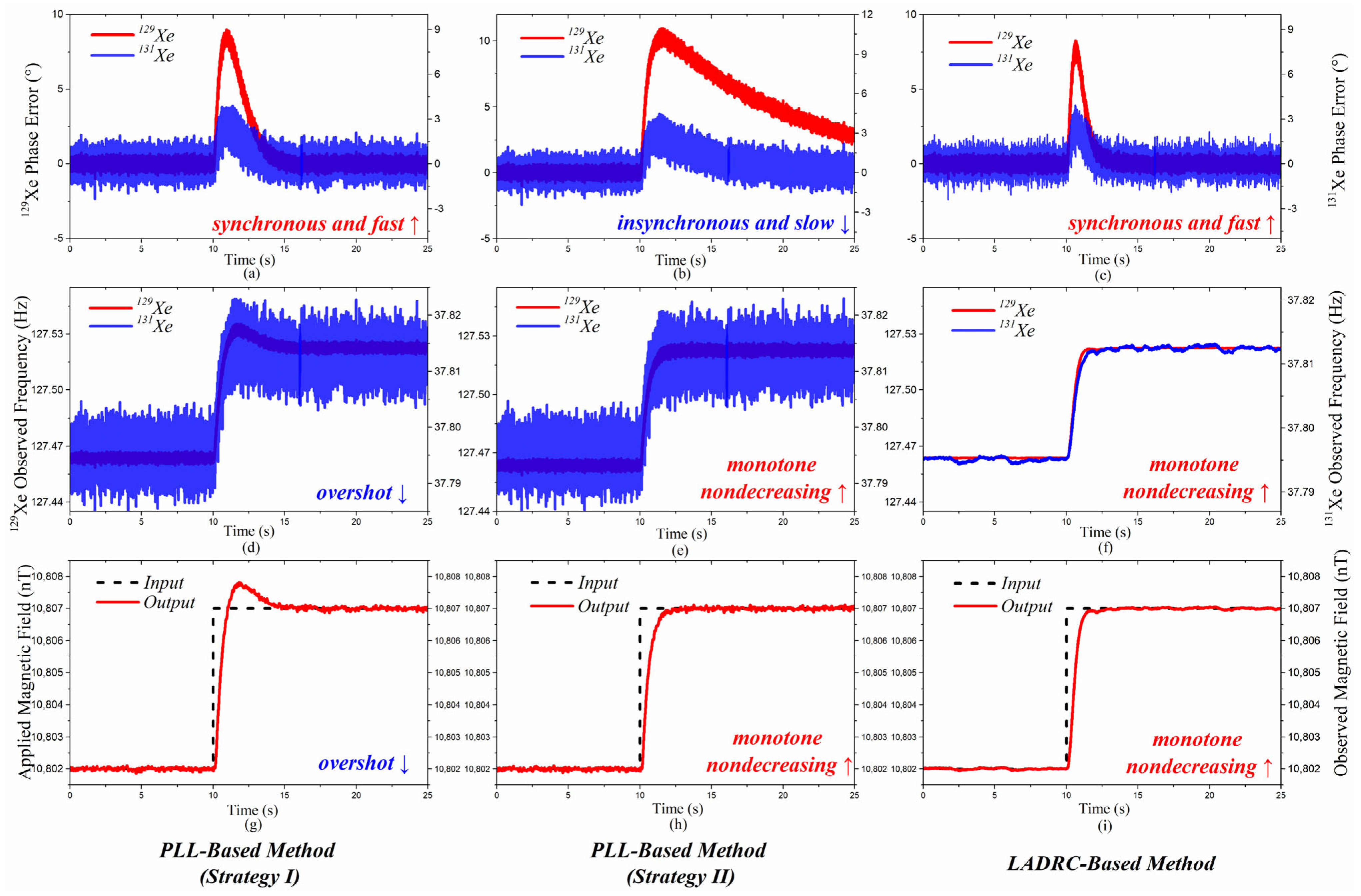
The experimental performance comparison is presented in Figure 5. Figure 5a–c are the phase-loop responses of the tested method. Figure 5d–f are the frequency-loop responses of the tested method. Figure 5g–i are the observed magnetic fields of the tested method calculated by the frequency observed from the frequency loops (the results of the PLL-based methods need to be filtered by a low-pass filter).
Figure 5.
Experimental performance of the PLL-based and LADRC-based methods with a step input signal. (a–c) are the phase-loop step response comparisons, (d–f) are the frequency-loop step response comparisons and (g–i) are the observed magnetic field.
It is obvious that the PLL-based method with parameter strategy I controlled the phases of two isotopes coherently as is shown in Figure 5a. In Figure 5b, the PLL-based method with parameter strategy II performed weakly on synchronization because the lifetime of the 129Xe is longer than the 131Xe. The results in Figure 5d,g show that great overshot appeared in the test of the parameter strategy I, which leads to great transient errors in the magnetic field measurement. Figure 5e,h show that strategy II has a great advantage in frequency observation. The overshot was suppressed and a monotone nondecreasing step response was obtained.
The LADRC-based method combined the advantages of both, as is shown in Figure 5c,f,i. The issue is decoupled in that the phase is controlled by LADRC, and the frequency is observed by LESO. The fast synchronous tracking phase loop and monotone nondecreasing frequency loop can be achieved at the same time, which is impossible for the PLL-based method.
5.2. Parameter Tuning of LADRC-Based Methods
In this experiment, the parameter tuning of the proposed LADRC-based method was considered.
Considering the system in Equation (13), the system parameter can be identified by a free inducing decay experiment. According to corollary 1, the parameter can be set as . Thus, only two parameters and need to be tuned. The influence of the two parameters were tested here.
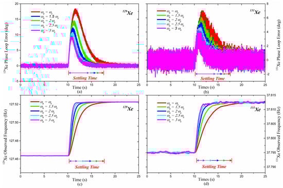
In Figure 6, the parameter was fixed to 3 mHz/deg ( Hz), and the parameter was set from 1~3 . A step input signal (5 nT) was added to the magnetic field of the z-axis, and the responses of both loops were recorded. Figure 6a,b show that the bandwidth of the LESO directly affects the phase-tracking performance, Figure 6c,d show its influence on frequency-observing, and Table 2 is the settling times of the experiments. The settling time of both loops is obviously reduced with a wider bandwidth. However, the bandwidth of LESO cannot be infinite due to the digital sampling and delay. According to the tests carried out in this paper, the bandwidth could be set to 3 (a faster feedback loop may be unstable) to obtain an acceptable feedback system.
Figure 6.
Experimental results of increasing bandwidth of the LESOs. (a,c) are the performance of the 129Xe, and (b,d) are the loop of 131Xe. Both kinds of isotopes were driven synchronously, and the influence of the parameter was specified.
Table 2.
Detailed Settling Time of the Tested Method in Figure 6.
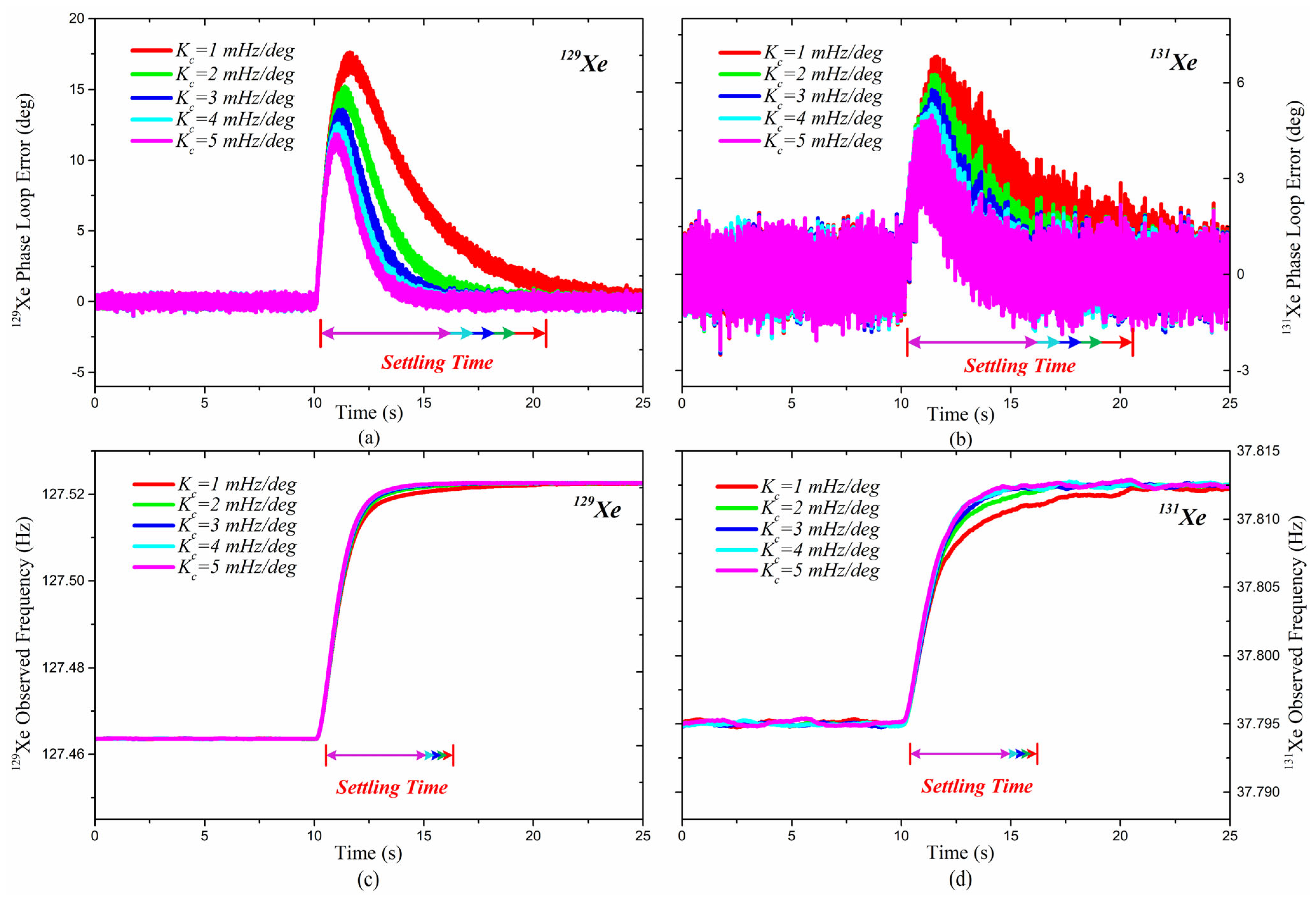
In Figure 7, the parameter was fixed to 2.16 Hz, and the parameter was set from 1~5 mHz/deg. A step input signal (5 nT) was added to the magnetic field of the z-axis, and the responses of both loops were recorded. Figure 7a,b are the phase-tracking response signals, Figure 7c,d are the frequency-observing response signals of both isotopes, and Table 3 is the settling times of the experiments. As is shown in the test results, played a dominant role in the phase-loop response, but not in the frequency-loop.
Figure 7.
Experimental results of increasing bandwidth of the LADRCs. (a,c) are the performance of the 129Xe, and (b,d) are the loop of 131Xe. Both kind of isotopes were driven synchronously, and the influence of the parameter was specified.
Table 3.
Detailed Settling Time of the Tested Method in Figure 7.
Consequently, the two unknown parameters are crucial to the performance of the LADRC-based magnetic field measurement.
- determines the frequency-observing performance significantly.
- Both and affect the phase-tracking performance.
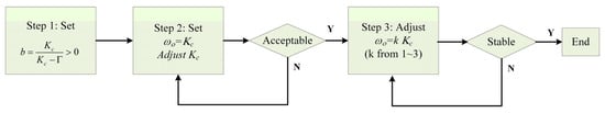
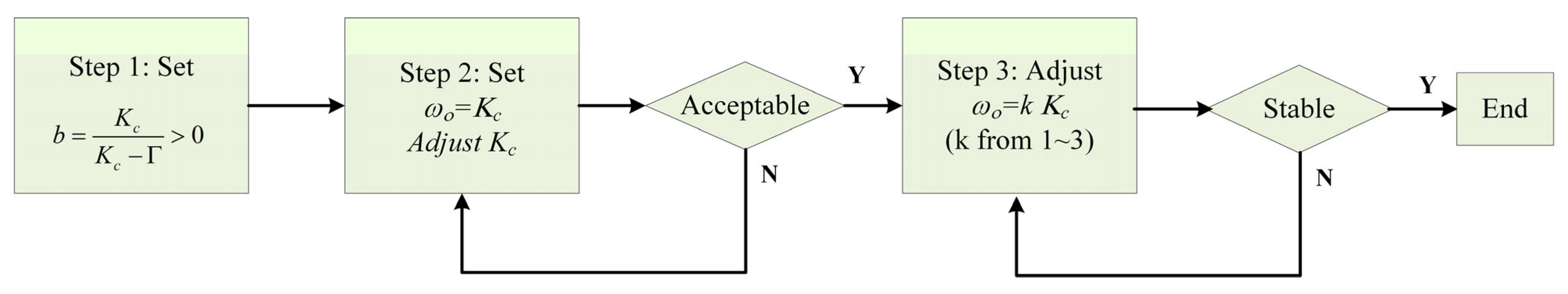
Therefore, a detailed parameter tuning process shown in Figure 8 is given as follows:
Figure 8.
Parameter tuning scheme of LADRC-based magnetic-field measurement method.
Step 1: Set for a monotone nondecreasing step response.
Step 2: Set , adjust to make the settling time of the loop acceptable.
Step 3: Adjust the bandwidth of LESO with a fixed . Find the largest based on the premise that the observer is stable.
6. Conclusions
This paper proposed a LADRC-based synchronous magnetic field measurement method for NMRRS. To provide a solution for improving the transient performance of the phase loop and frequency loop synchronously. LADRCs have been utilized to control the dual nuclear spins which precess synchronously, and the magnetic field fluctuations were observed by the LESOs. An experimental NMRRS was constructed. The effectiveness was demonstrated through mathematical analysis and comparative experimental results. Compared with the existing PLL-based magnetic field measurement method, the proposed method has several advantages, as follows:
- (1)
- the proposed LADRC-based method controls the phase loops of the two nuclear spins synchronously, which is fundamental for transient error suppression.
- (2)
- the proposed method has an outstanding performance in providing a monotone, nondecreasing step response of observing Larmor frequency, which is achieved without any destruction in the phase-tracking of the two isotopes.
- (3)
- the parameter tuning process of the proposed method is simple and fast; most of them can be calculated for a certain known cell.
The proposed method is suitable for NMRRS applications which suffer from complicated external magnetic field environments. The methods proposed may be applied to other frequency measurements of controlled oscillators elsewhere.
Author Contributions
Conceptualization, X.Z. and X.S.; methodology, X.Z.; software, Y.S. and X.Z.; validation, X.Z. and Y.S.; formal analysis, X.Z.; investigation, X.Z. and Y.S.; resources, X.Z.; data curation, X.Z. and Y.S.; writing—original draft preparation, X.Z.; writing—review and editing, X.S.; visualization, X.Z.; supervision, J.L.; project administration, Z.L.; funding acquisition, J.L. and Z.L. All authors have read and agreed to the published version of the manuscript.
Funding
This work was funded by the National Key Research and Development Program of China under Grand 2018YFB2002404, National Natural Science Foundation of China (NSFC) under Grant 61421063, Grant 61873020 and Grant 62003022.
Institutional Review Board Statement
Not applicable.
Informed Consent Statement
Not applicable.
Data Availability Statement
Data sharing is not applicable.
Conflicts of Interest
The authors declare no conflict of interest.
References
- Kitching, J.; Knappe, S.; Donley, E.A. Atomic Sensors—A Review. IEEE Sens. J. 2011, 11, 1749–1758. [Google Scholar]
- Degen, C.L.; Reinhard, F.; Cappellaro, P. Quantum sensing. Rev. Mod. Phys. 2017, 89, 035002. [Google Scholar] [CrossRef] [Green Version]
- Feng, D. Review of Quantum navigation. IOP Conf. Ser. Earth Environ. Sci. 2019, 237, 032027. [Google Scholar] [CrossRef]
- Fang, J.; Qin, J. Advances in Atomic Gyroscopes: A View from Inertial Navigation Applications. Sensors 2012, 12, 6331–6346. [Google Scholar] [CrossRef]
- Meyer, D.; Larsen, M. Nuclear magnetic resonance gyro for inertial navigation. Gyroscopy Navig. 2014, 5, 75–82. [Google Scholar] [CrossRef]
- Walker, T.G.; Larsen, M.S. Spin-Exchange-Pumped NMR Gyros. In Advances in Atomic, Molecular, and Optical Physics; Elsevier: Amsterdam, The Netherlands, 2016; Volume 65, pp. 373–401. ISBN 978-0-12-804828-3. [Google Scholar]
- Woodman, K.F.; Franks, P.W.; Richards, M.D. The Nuclear Magnetic Resonance Gyroscope: A Review. J. Navig. 1987, 40, 366–384. [Google Scholar]
- Larsen, M.; Bulatowicz, M. Nuclear magnetic resonance gyroscope: For DARPA’s micro-technology for positioning, navigation and timing program. In 2012 IEEE International Frequency Control Symposium Proceedings; IEEE: Piscataway, NJ, USA, 2014. [Google Scholar]
- Chow, W.W.; Gea-Banacloche, J.; Pedrotti, L.M.; Sanders, V.E.; Schleich, W.; Scully, M.O. The ring laser gyro. Rev. Mod. Phys. 1985, 57, 61–104. [Google Scholar]
- Bergh, R.A.; Lefevre, H.C.; Shaw, H.J. All-single-mode fiber-optic gyroscope. Opt. Lett. 1981, 6, 198–200. [Google Scholar]
- Schwindt, P.D.D.; Knappe, S.; Shah, V.; Hollberg, L.; Kitching, J.; Liew, L.-A.; Moreland, J. Chip-scale atomic magnetometer. Appl. Phys. Lett. 2004, 85, 6409–6411. [Google Scholar] [CrossRef]
- Knappe, S.; Schwindt, P.D.D.; Shah, V.; Hollberg, L.; Kitching, J.; Liew, L.; Moreland, J. A chip-scale atomic clock based on ^87Rb with improved frequency stability. Opt. Express 2005, 13, 1249–1253. [Google Scholar] [CrossRef]
- Donley, E.A. Nuclear magnetic resonance gyroscopes. In Proceedings of the 2010 IEEE SENSORS, Waikoloa, HI, USA, 1–4 November 2010; pp. 17–22. [Google Scholar]
- Zhang, D.-W.; Xu, Z.-Y.; Zhou, M.; Xu, X.-Y. Parameter analysis for a nuclear magnetic resonance gyroscope based on 133Cs–129Xe/131Xe. Chin. Phys. B 2017, 26, 023201. [Google Scholar]
- Vershovskii, A.K.; Litmanovich, Y.A.; Pazgalev, A.S.; Peshekhonov, V.G. Nuclear Magnetic Resonance Gyro: Ultimate Parameters. Gyroscopy Navig. 2018, 9, 162–176. [Google Scholar] [CrossRef]
- Zhang, K.; Zhao, N.; Wang, Y.-H. Closed-Loop Nuclear Magnetic Resonance Gyroscope Based on Rb-Xe. Sci. Rep. 2020, 10, 2258. [Google Scholar] [CrossRef] [Green Version]
- Simpson, J.H.; Fraser, J.T.; Greenwood, I.A. An Optically Pumped Nuclear Magnetic Resonance Gyroscope. IEEE Trans. Aerosp. 1963, 1, 1107–1110. [Google Scholar] [CrossRef]
- Karwacki, F.A. Nuclear Magnetic Resonance Gyro Development. Navigation 1980, 27, 72–78. [Google Scholar] [CrossRef]
- Han, J. From PID to Active Disturbance Rejection Control. IEEE Trans. Ind. Electron. 2009, 56, 900–906. [Google Scholar] [CrossRef]
- Gao, Z. Scaling and bandwidth-parameterization based controller tuning. In Proceedings of the 2003 American Control Conference, Denver, CO, USA, 4–6 June 2003; IEEE: Denver, CO, USA, 2003; Volume 6, pp. 4989–4996. [Google Scholar]
- Sun, G.; Li, Y.; Jin, W.; Bu, L. A Nonlinear Three-Phase Phase-Locked Loop Based on Linear Active Disturbance Rejection Controller. IEEE Access 2017, 5, 21548–21556. [Google Scholar] [CrossRef]
- Guo, B.; Bacha, S.; Alamir, M.; Hably, A.; Boudinet, C. Generalized Integrator-Extended State Observer With Applications to Grid-Connected Converters in the Presence of Disturbances. IEEE Trans. Contr. Syst. Technol. 2021, 29, 744–755. [Google Scholar] [CrossRef]
- Guo, B.; Bacha, S.; Alamir, M.; Pouget, J. A phase-locked loop using ESO-based loop filter for grid-connected converter: Performance analysis. Control Theory Technol. 2021, 19, 49–63. [Google Scholar] [CrossRef]
- Yang, R.; Sun, M.; Chen, Z. Active disturbance rejection control on first-order plant. J. Syst. Eng. Electron. 2011, 22, 8. [Google Scholar] [CrossRef]
- Lin, S.-K.; Fang, C.-J. Nonovershooting and monotone nondecreasing step responses of a third-order SISO linear system. IEEE Trans. Automat. Contr. 1997, 42, 1299–1303. [Google Scholar]


Publisher’s Note: MDPI stays neutral with regard to jurisdictional claims in published maps and institutional affiliations. |
© 2021 by the authors. Licensee MDPI, Basel, Switzerland. This article is an open access article distributed under the terms and conditions of the Creative Commons Attribution (CC BY) license (https://creativecommons.org/licenses/by/4.0/).