
Kinematic Analysis and Motion Planning of Cable-Driven Rehabilitation Robots


Abstract
:1. Introduction
2. Structure of Rehabilitation Robot and Human Lower Limb Model
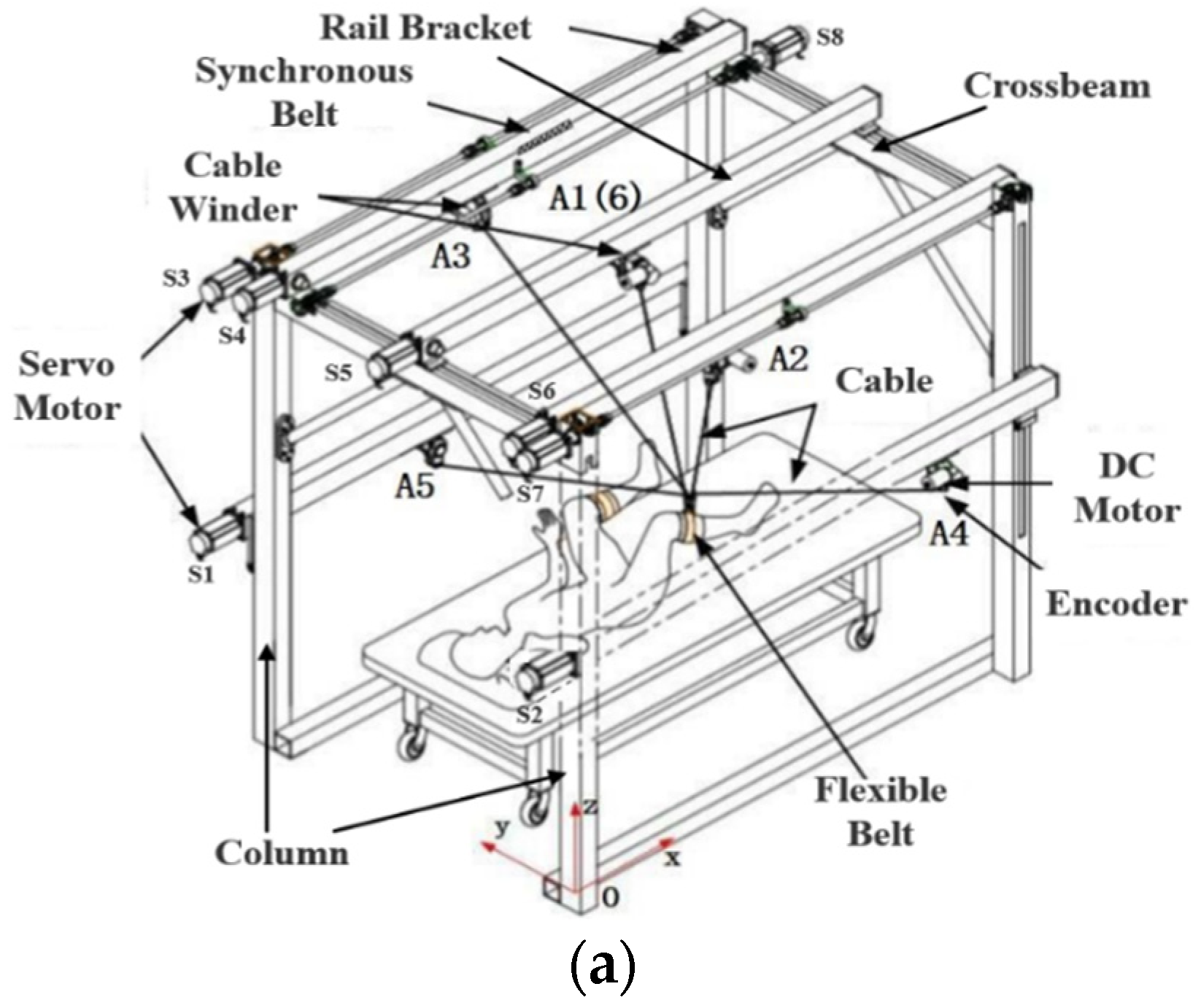
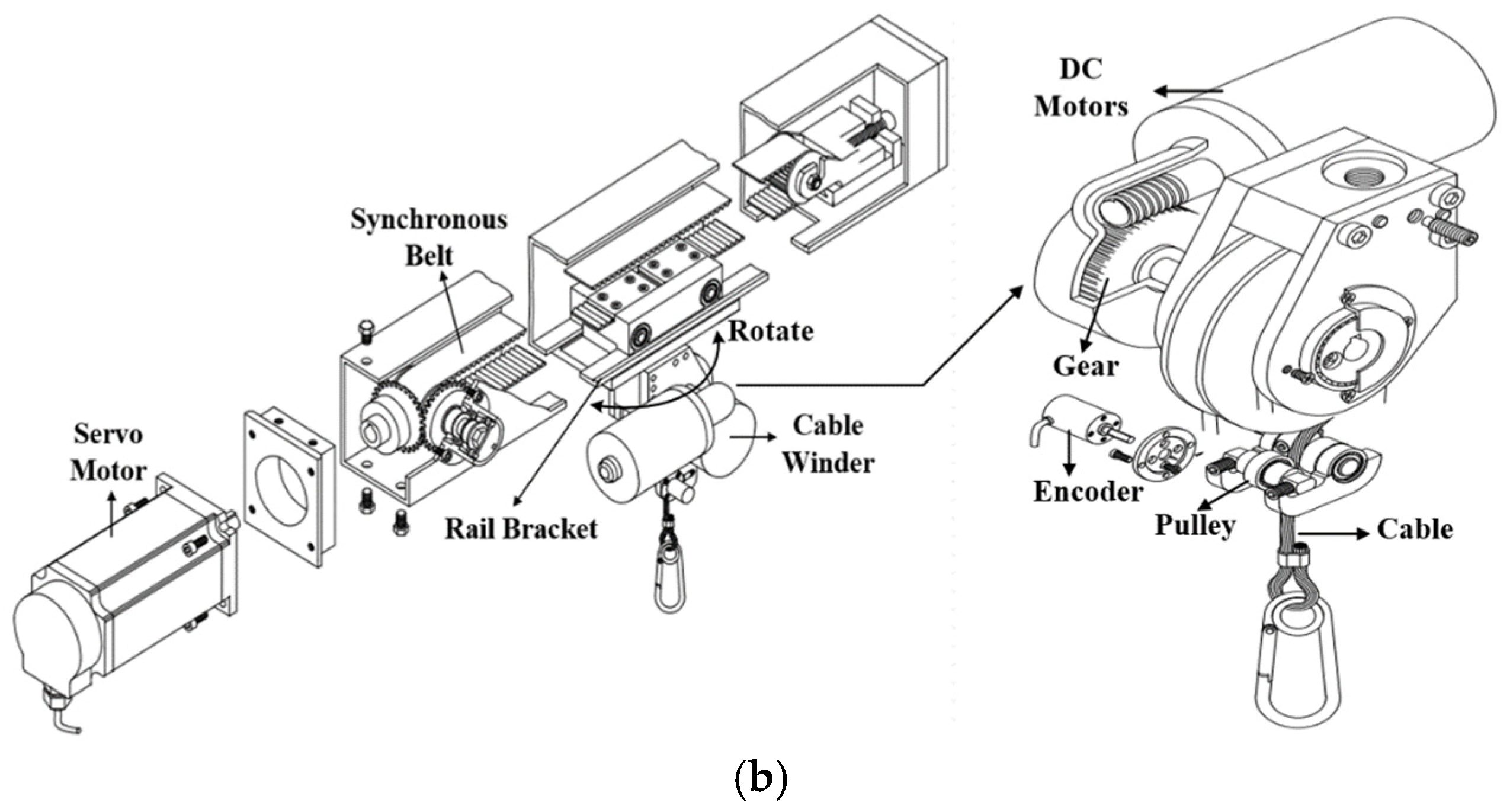
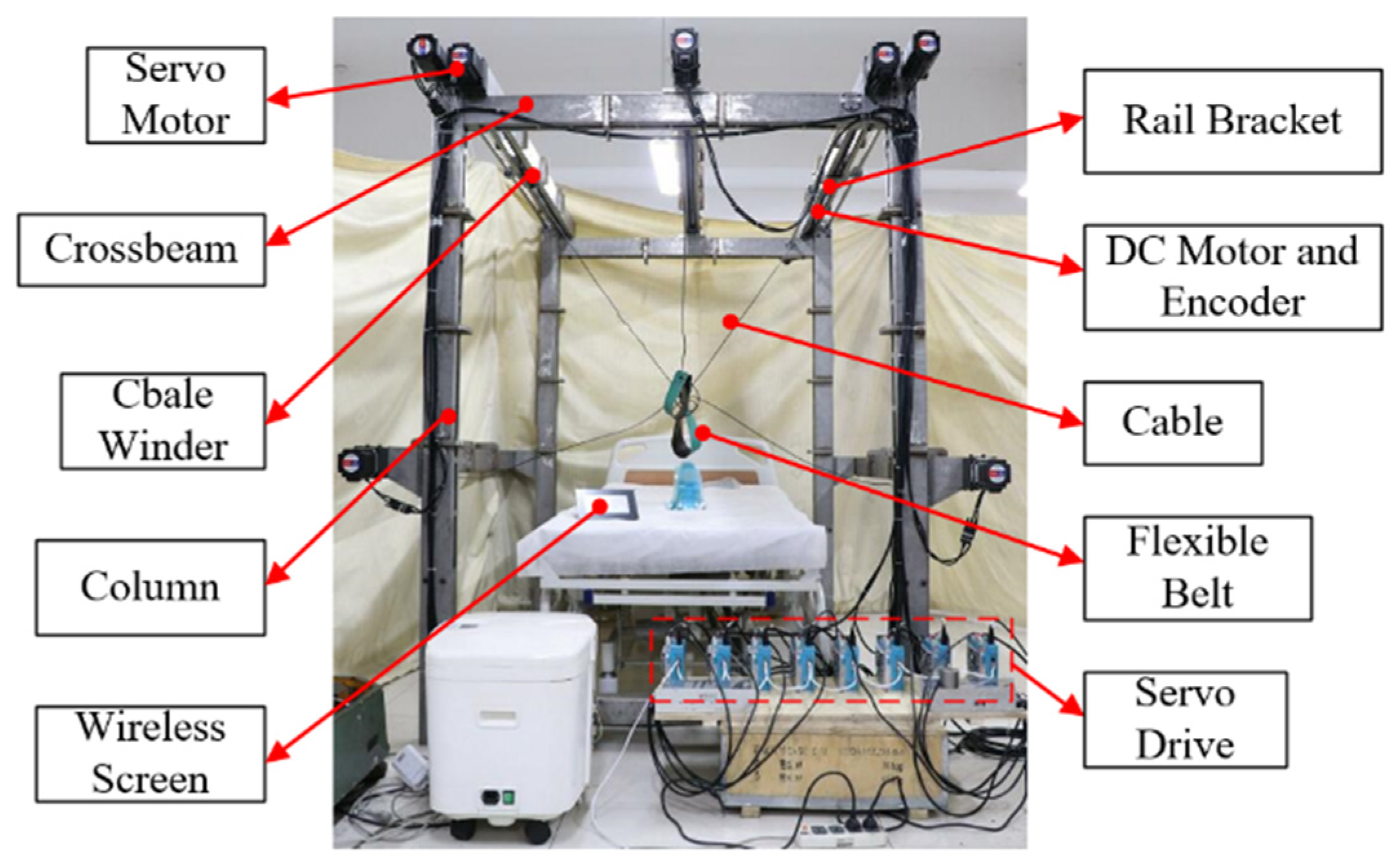
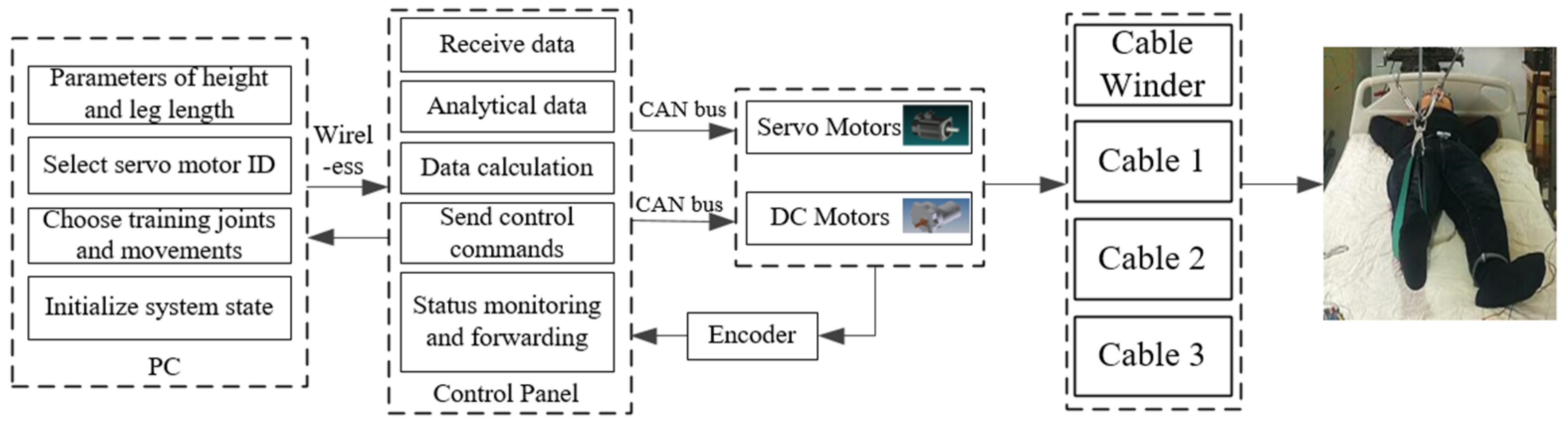
2.1. Structure of Robot
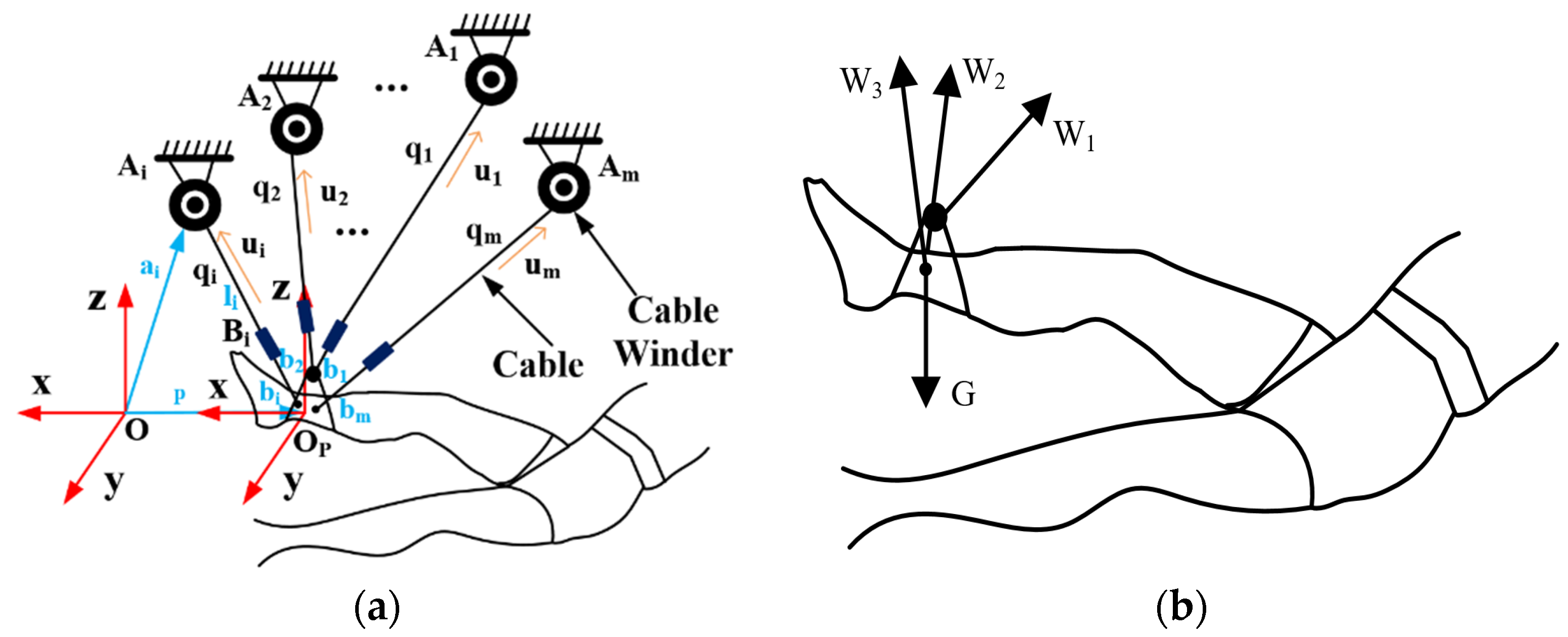
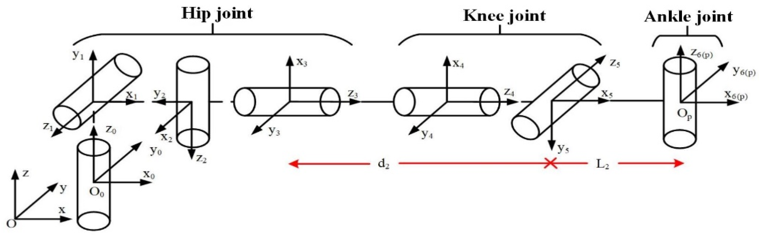
2.2. Human Lower Limb Model
3. Kinematics Analysis of Rehabilitation Robot
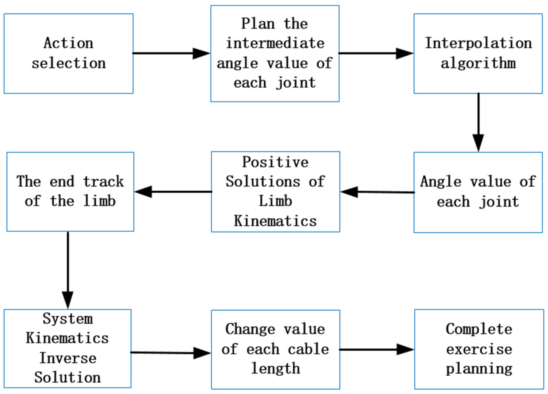
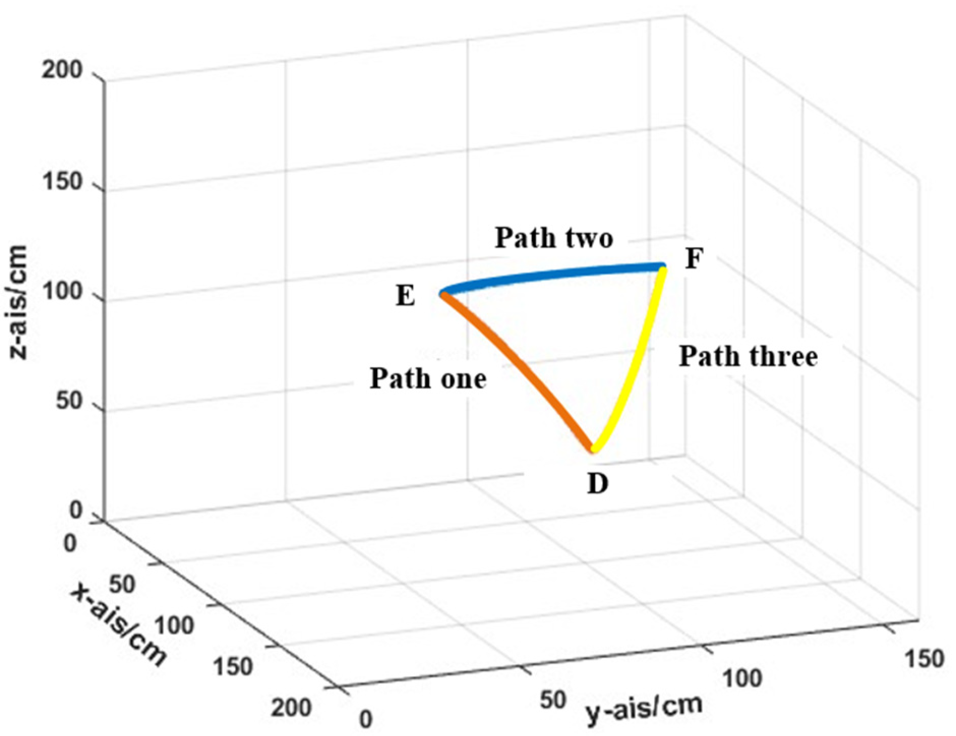
4. Trajectory Planning
4.1. Adaptive S-Shaped Speed Curve
4.2. Polynomial Programming Based on S-Shaped Curve
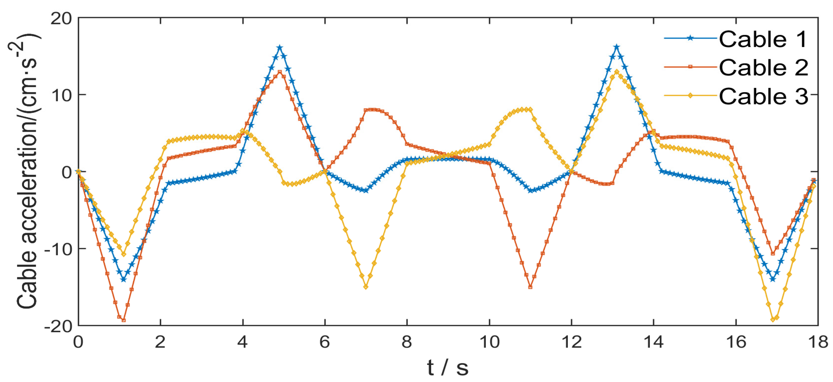
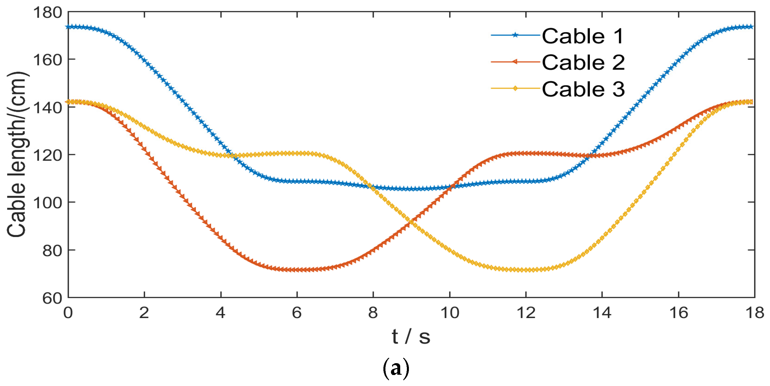
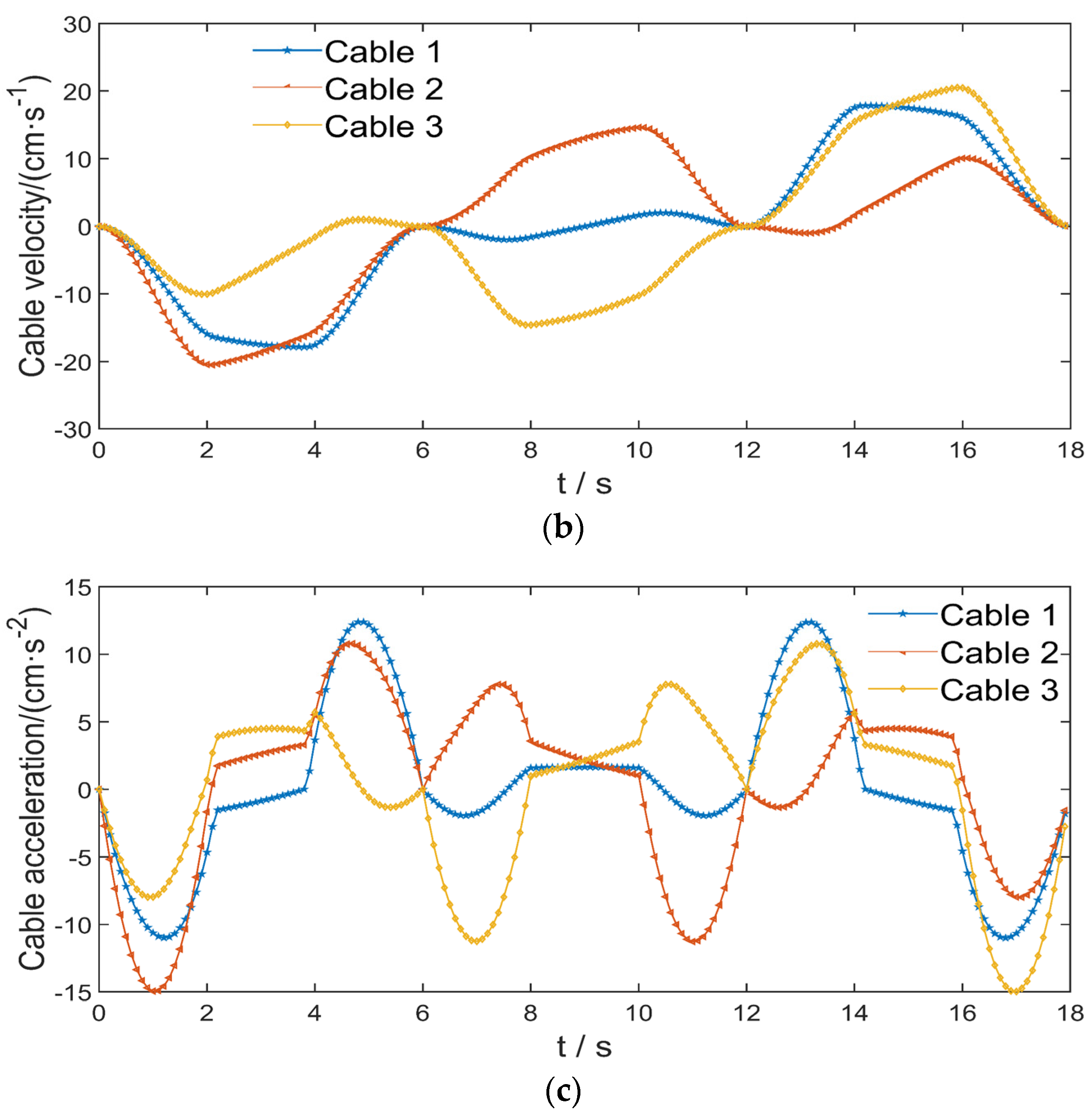
5. Simulation Results
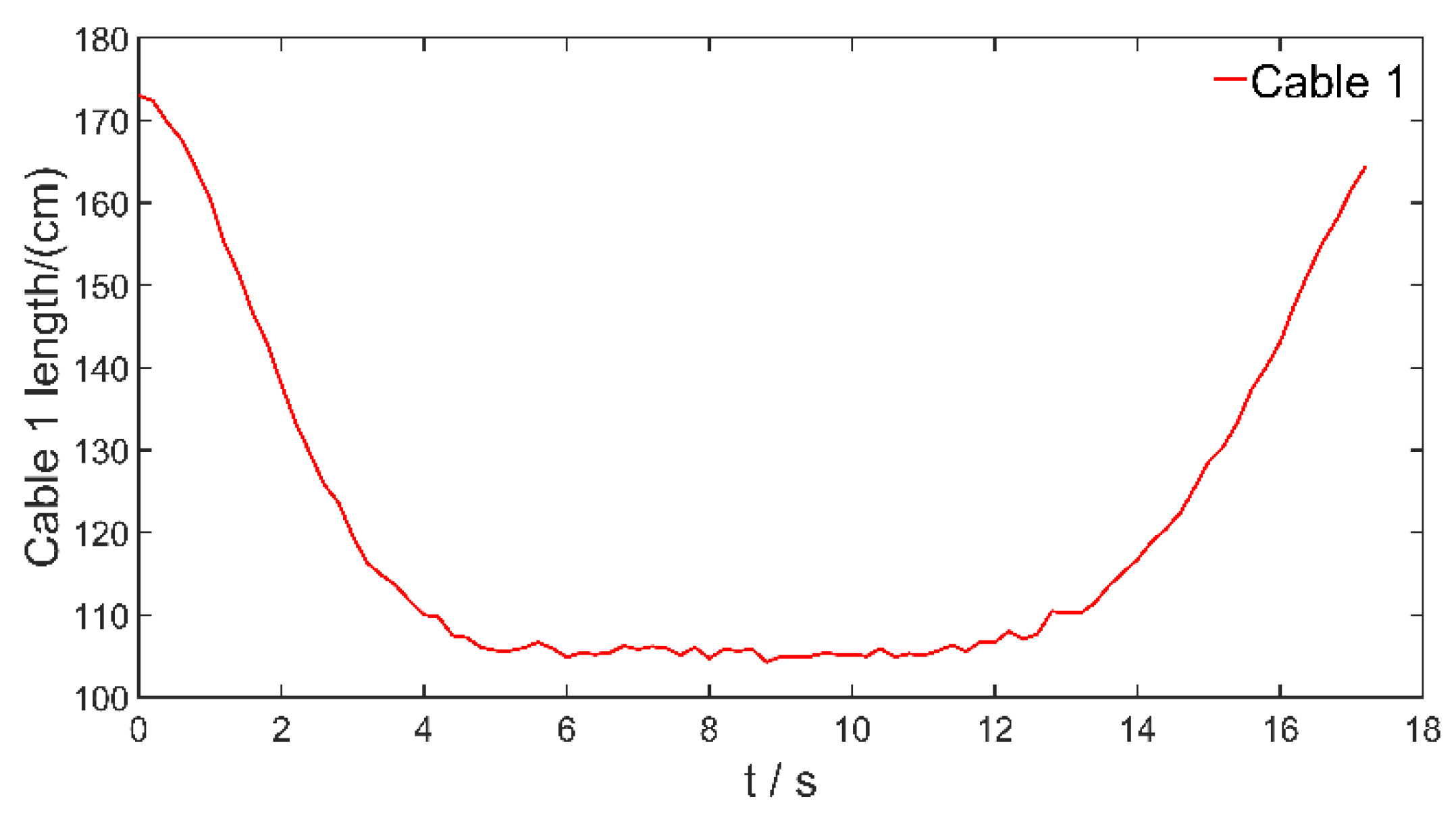
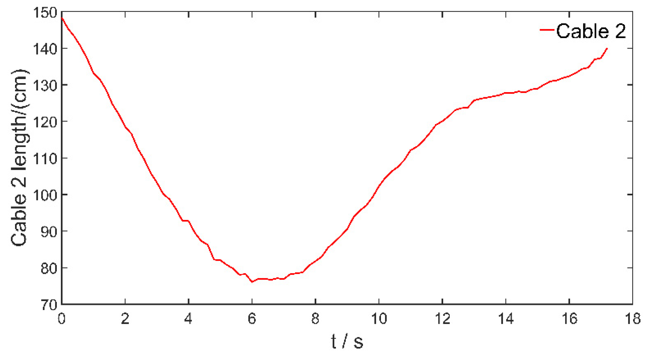
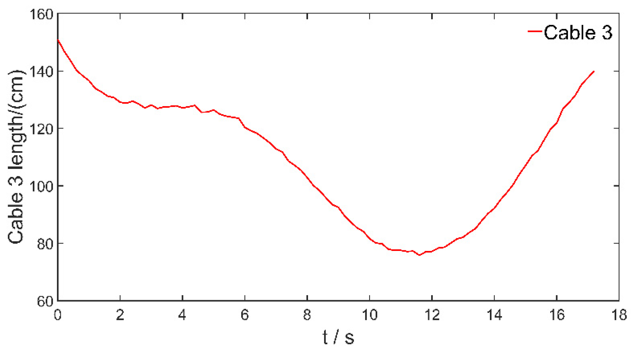
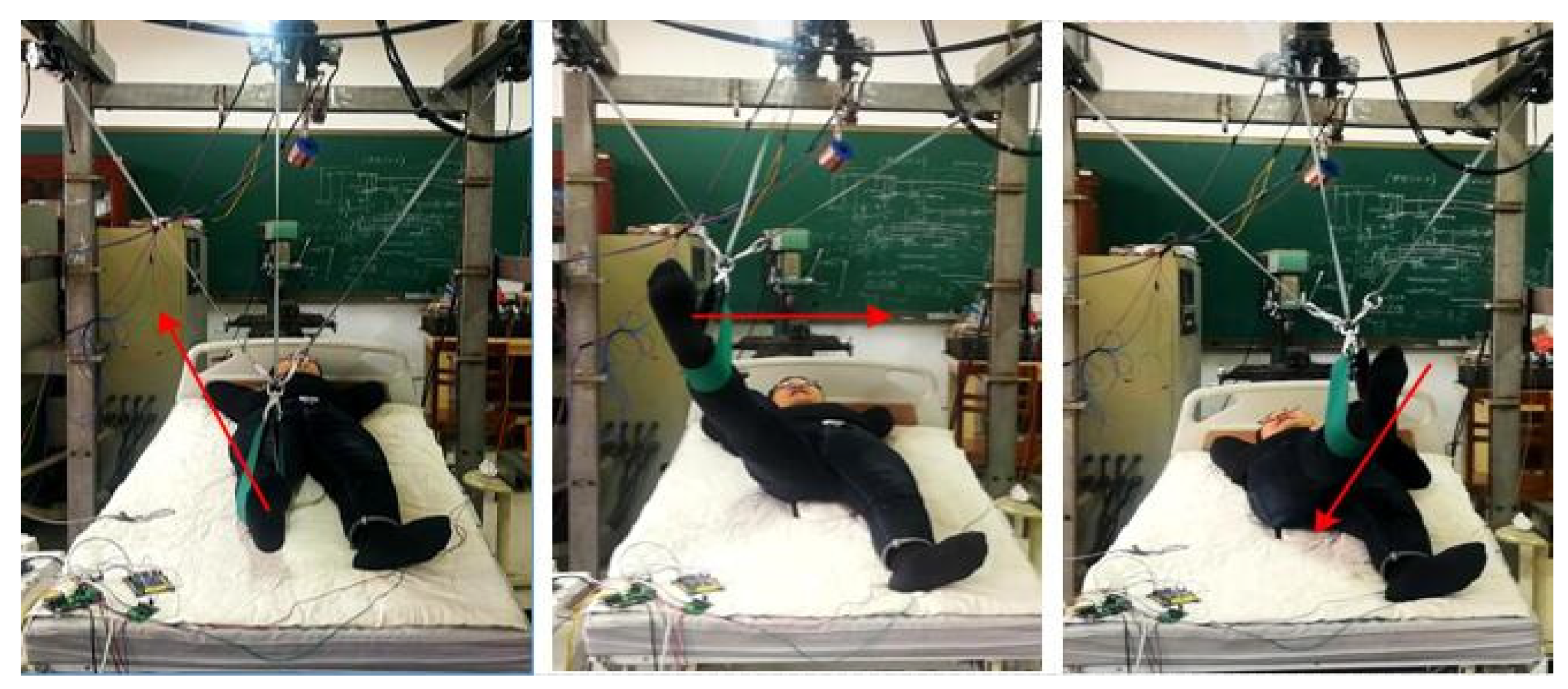
6. Experiments of Rehabilitation Robot
7. Conclusions
Author Contributions
Funding
Institutional Review Board Statement
Informed Consent Statement
Conflicts of Interest
References
- Chen, B.; Ma, H.; Yin, L.; Gao, F.; Chan, K.-M.; Law, S.-W.; Qin, L.; Liao, W.-H. Recent developments and challenges of lower extremity exoskeletons. J. Orthop. Transl. 2016, 5, 26–37. [Google Scholar] [CrossRef] [Green Version]
- Wang, Y.-L.; Wang, K.-Y.; Zhao, W.-Y.; Wang, W.-L.; Han, Z.; Zhang, Z.-X. Effects of single crouch walking gaits on fatigue damages of lower extremity main muscles. J. Mech. Med. Biol. 2019, 19, 1940046. [Google Scholar] [CrossRef] [Green Version]
- Zhao, Y.N.; Hao, Z.W.; Li, J.M. The effect of lokomat lower limb gait training rehabilitation robot on balance function and walking ability in hemiplegic patients after ischemic stroke. Chin. J. Rehabil. Med. 2012, 27, 1015–1020. [Google Scholar]
- Gazi, A.; Ahmet, E.C.; Erkan, K. Exoskeleton design and adaptive compliance control for hand rehabilitation. Trans. Inst. Meas. Control. 2019, 42, 493–502. [Google Scholar]
- Reinkensmeyer, D.J.; Boninger, M.L. Technologies and combination therapies for enhancing movement training for people with a disability. J. Neuroeng. Rehabil. 2012, 9, 17. [Google Scholar] [CrossRef] [PubMed] [Green Version]
- Wang, K.; Yin, P.; Yang, H.; Wang, L. Motion planning of rigid chain for rigid-flexible coupled robot. Int. J. Adv. Robot. Syst. 2018, 15, 1729881418772815. [Google Scholar] [CrossRef]
- Nef, T.; Guidali, M.; Klamroth-Marganska, V.; Riener, R. ARMin-exoskeleton robot for stroke rehabilitation. IFMBE Proc. 2009, 25, 127–130. [Google Scholar]
- Jian, H.; Tu, X.; He, J. Design and evaluation of the RUPERT wearable upper extremity exoskeleton robot for clinical and in-home therapies. IEEE Trans. Syst. Man Cybern. Syst. 2016, 46, 926–935. [Google Scholar]
- Perry, J.C.; Rosen, J. Upper-limb powered exoskeleton design. IEEE/ASME Trans. Mechatron. 2007, 12, 408–417. [Google Scholar] [CrossRef]
- Chen, S.H.; Lien, W.-M.; Wang, W.-W.; Lee, G.-D.; Hsu, L.-C.; Lee, K.-W.; Lin, S.-Y.; Lin, C.-H.; Fu, L.-C.; Lai, J.-S.; et al. Assistive control system for upper limb rehabilitation robot. IEEE Trans. Neural Syst. Rehabil. Eng. 2016, 24, 1199–1209. [Google Scholar] [CrossRef]
- Ugurlu, B.; Nishimura, M.; Hyodo, K.; Kawanishi, M.; Narikiyo, T. Proof of concept for robot-aided upper limb rehabilitation using disturbance observers. IEEE Trans. Hum. -Mach. Syst. 2015, 45, 110–118. [Google Scholar] [CrossRef]
- Rathore, A.; Wilcox, M.; Ramirez, D.Z.M.; Loureiro, R.; Carlson, T. Quantifying the human-robot interaction forces between a lower limb exoskeleton and healthy users. In Proceedings of the 2016 38th Annual International Conference of the IEEE Engineering in Medicine and Biology Society (EMBC), Orlando, FL, USA, 16–20 August 2016; pp. 586–589. [Google Scholar]
- Cao, L.; Tang, X.Q.; Wang, W.F. Tension optimization and experimental research of parallel mechanism driven by 8 cables for constant vector force output. Robot 2015, 37, 641–647. [Google Scholar]
- Wang, W.F.; Tang, X.Q.; Shao, Z.F. Design and analysis of a wire-driven parallel mechanism for large vertical storage tank. J. Mech. Eng. 2016, 52, 1–8. [Google Scholar]
- Zhang, B.; Shang, W.W.; Cong, S.; Li, Z. Coordinated dynamic control in the task space for redundantly actuated cable-driven parallel robots. IEEE/ASME Trans. Mechatron. 2020, 26, 2396–2407. [Google Scholar] [CrossRef]
- Ming, W.; Hornby, T.G.; Landry, J.M.; Roth, H.; Schmit, B.D. A cable-driven locomotor training system for restoration of gait in human SCI. Gait Posture 2011, 33, 256–260. [Google Scholar]
- Wang, Y.L.; Wang, K.-y.; Zhang, Z.-x.; Han, Z.; Wang, W.-l. Analysis of dynamical stability of rigid-flexible hybrid-driven lower limb rehabilitation robot. J. Mech. Sci. Technol. 2020, 34, 1735–1748. [Google Scholar] [CrossRef]
- Ennaiem, F.; Chaker, A.; Laribi, M.A.; Sandoval, J.; Bennour, S.; Mlika, A.; Romdhane, L.; Zeghloul, S. Task-Based Design Approach: Development of a Planar Cable-Driven Parallel Robot for Upper Limb Rehabilitation. Appl. Sci. 2021, 11, 5635. [Google Scholar] [CrossRef]
- Yang, Z.M.; Zi, B.; Chen, B. Mechanism Design and Kinematic Analysis of a Waist and Lower Limbs Cable-Driven Parallel Rehabilitation Robot. In Proceedings of the IEEE 3rd Advanced Information Management, Communicates, Electronic and Automation Control Conference, Chongqing, China, 11–13 October 2019; IEEE: Chongqing, China, 2019; pp. 723–727. [Google Scholar]
- Wang, Y.L.; Wang, K.Y.; Zhang, Z.X. Design, comprehensive evaluation, and experimental study of a cable-driven parallel robot for lower limb rehabilitation. J. Braz. Soc. Mech. Sci. Eng. 2020, 42, 1735–1748. [Google Scholar] [CrossRef]
- Rogério, S.G.; Carvalho, J.; Rodrigues, L.A.O.; Barbosa, A.M. Cable-Driven Parallel Manipulator for Lower Limb Rehabilitation. Appl. Mech. Mater. 2014, 2828, 535–542. [Google Scholar]
- Wang, K.-Y.; Yin, P.-C.; Yang, H.-P.; Tang, X.-Q. The man-machine motion planning of rigid-flexible hybrid lower limb. Adv. Mech. Eng. 2018, 10, 1687814018775865. [Google Scholar]
- Ghasem, A.; Jungwon, Y.; Hosu, L. Optimum kinematic design of a planar cable-driven parallel robot with wrench-closure gait trajectory. Mech. Mach. Theory 2016, 99, 1–18. [Google Scholar]
- Rosati, G.; Zanotto, D.; Agrawal, S.K. On the design of adaptive cable-driven systems. J. Mech. Robot. 2011, 3, 021004. [Google Scholar] [CrossRef]
- Nguyen, D.Q.; Gouttefarde, M. Study of Reconfigurable Suspended Cable-Driven Parallel Robots for Airplane Maintenance. In Proceedings of the 2014 IEEE/RSJ International Conference on Intelligent Robots and Systems, Chicago, IL, USA, 14–18 November 2014; pp. 14–18. [Google Scholar]
- Gagliardini, L.; Caro, S.; Gouttefarde, M.; Girin, A. Discrete reconfiguration planning for cable-driven parallel robots. Mech. Mach. Theory 2016, 100, 313–337. [Google Scholar] [CrossRef] [Green Version]
- Rosati, G.; Andreolli, M.; Biondi, A.; Gallina, P. Performance of cable suspended robots for upper limb rehabilitation. In Proceedings of the IEEE 10th International Conference on Rehabilitation Robotics (ICORR), Noordwijk, The Netherlands, 13–15 June 2007; pp. 13–15. [Google Scholar]
- Mao, Y.; Agrawal, S.K. Design of a cable-driven arm exoskeleton (CAREX) for neural rehabilitation. IEEE Trans. Robot. 2012, 28, 922–931. [Google Scholar] [CrossRef]
- Zanotto, D.; Rosati, G.; Minto, S.; Rossi, A. Sophia-3: A semiadaptive cable-driven rehabilitation device with a tilting working plane. IEEE Trans. Robot. 2014, 30, 974–979. [Google Scholar] [CrossRef]
- Kim, H.; Miller, L.M.; Fedulow, I.; Simkins, M.; Abrams, G.M.; Byl, N.; Rosen, J. Kinematic data analysis for post-stroke patients following bilateral versus unilateral rehabilitation with an upper limb wearable robotic system. IEEE Trans. Neural Syst. Rehabil. Eng. 2013, 21, 153–164. [Google Scholar] [CrossRef] [PubMed]
- Rezazadeh, S.; Behzadipour, S. Workspace analysis of multibody cable-driven mechanisms. ASME J. Mech. Robot. 2011, 3, 021005. [Google Scholar] [CrossRef]
- Lau, D.; Oetomo, D.; Halgamuge, S.K. Generalized modeling of multilink cable-driven manipulators with arbitrary routing using the cable-routing matrix. IEEE Trans. Robot. 2013, 5, 1102–1113. [Google Scholar] [CrossRef]
- Niku, S.B. Introduction to Robotics: Analysis, Systems, Application; Pearson Education: Upper Saddle River, NJ, USA, 2011. [Google Scholar]
- Pan, H.J.; Ma, C.H.; Shen, S.F. Study on the maximum motion range of main joints of human limbs. J. Zhejiang Norm. Univ. Nat. Sci. Ed. 1995, 3, 64–68. [Google Scholar]
- Strydom, M.L.; Banach, A.; Roberts, J.; Crawford, R.; Jaiprakash, A.T. Kinematic Model of the Human Leg Using DH Parameters. IEEE Access 2020, 8, 191737–191750. [Google Scholar] [CrossRef]
- Jung, Y.; Bae, J. Kinematic Analysis of a 5-DOF Upper-Limb Exoskeleton with a Tilted and Vertically Translating Shoulder Joint. IEEE/ASME Trans. Mechatron. 2015, 20, 1428–1439. [Google Scholar] [CrossRef]
- Khalipour, S.A.; Khorrambakht, R.; Taghirad, H.D.; Cardou, P. Robust cascade control of a deployable cable-driven robot. Mech. Syst. Signal Process. 2019, 127, 513–531. [Google Scholar] [CrossRef]
- Santos, J.C.; Chemori, A.; Gouttefarde, M. Model predictive control of large-dimension cable-driven parallel robots. Mech. Mach. Sci. 2019, 74, 221–232. [Google Scholar]
- Fang, S.; Cao, J.; Zhang, Z.; Zhang, Q.; Cheng, W. Study on High-Speed and Smooth Transfer of Robot Motion Trajectory Based on Modified S-shaped Acceleration/Deceleration Algorithm. IEEE Access 2020, 8, 199747–199758. [Google Scholar] [CrossRef]
- Saravanan, R.; Ramabalan, S. Evolutionary Minimum Cost Trajectory Planning for Industrial Robots. J. Intell. Robot. Syst. 2008, 52, 45–77. [Google Scholar] [CrossRef]
- Gasparetto, A.; Zanotto, V. A new method for smooth trajectory planning of robot manipulators. Mech. Mach. Theory 2007, 42, 455–471. [Google Scholar] [CrossRef]
- Wang, H.F.; Zhu, S.Q.; Wu, W.X. INSGA-II based multi-objective trajectory planning for manipulators. J. Zhejiang Univ. Eng. Sci. 2012, 46, 622–628. [Google Scholar]


| Human Joint | |||||
|---|---|---|---|---|---|
| 1 | 90 | 0 | 0 | 0–60 | |
| 2 | 90 | 0 | 0 | 60–135 | |
| 3 | 90 | 0 | 0 | −135 to −45 | |
| 4 | 0 | 0 | −10 to 10 | ||
| 5 | 90 | 0 | 0 | 90–210 | |
| 6 | 0 | 0 | −20 to 45 |
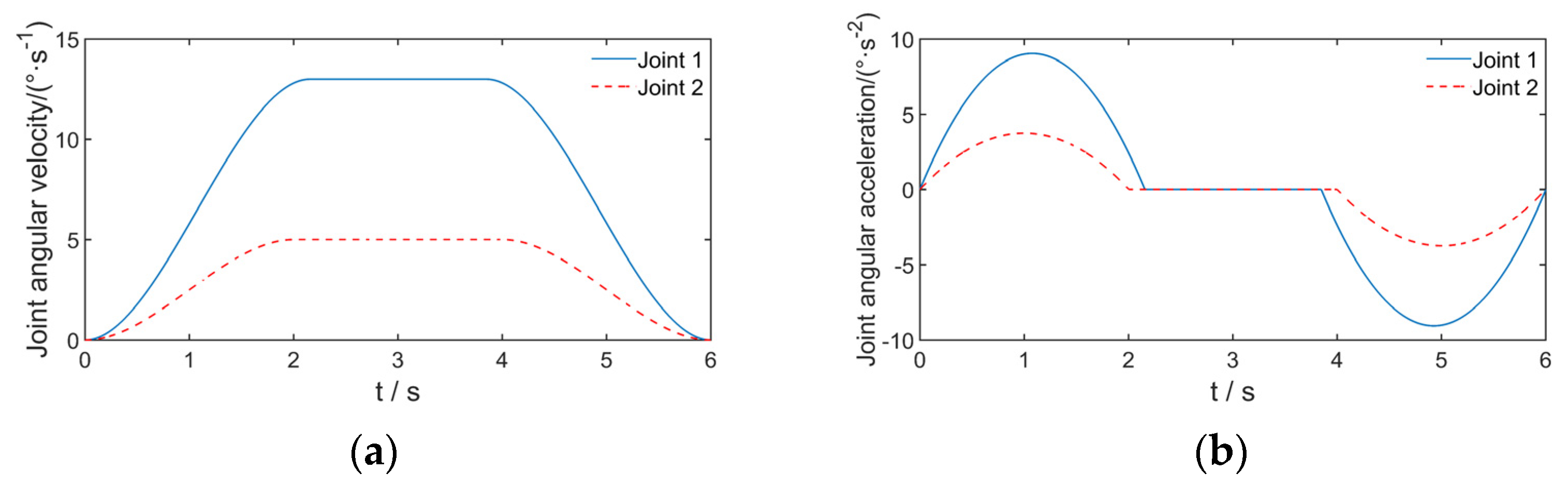
| Joint 1 | Angular | Maximum Angular | Maximum Angular |
|---|---|---|---|
| Path one | 0–50 | 13 | 25 |
| Path two | 50–50 | 0 | 0 |
| Path three | 50–0 | 13 | 25 |
| Joint 2 | Angular | Maximum Angular | Maximum Angular |
|---|---|---|---|
| Path one | 90–110 | 5 | 10 |
| Path two | 110–70 | 10 | 20 |
| Path three | 70–90 | 5 | 10 |
| Index | Fifth-Degree Polynomial Programming Based on S-Curve | S-Shaped Curve | Quintic Polynomial Programming |
|---|---|---|---|
| 5.8320 | 6.3689 | 7.4505 | |
| 27.8875 | 28.0933 | 29.8935 |
Publisher’s Note: MDPI stays neutral with regard to jurisdictional claims in published maps and institutional affiliations. |
© 2021 by the authors. Licensee MDPI, Basel, Switzerland. This article is an open access article distributed under the terms and conditions of the Creative Commons Attribution (CC BY) license (https://creativecommons.org/licenses/by/4.0/).
Share and Cite
Zhang, J.; Cao, D.; Wu, Y. Kinematic Analysis and Motion Planning of Cable-Driven Rehabilitation Robots. Appl. Sci. 2021, 11, 10441. https://doi.org/10.3390/app112110441
Zhang J, Cao D, Wu Y. Kinematic Analysis and Motion Planning of Cable-Driven Rehabilitation Robots. Applied Sciences. 2021; 11(21):10441. https://doi.org/10.3390/app112110441
Chicago/Turabian StyleZhang, Jingyu, Dianguo Cao, and Yuqiang Wu. 2021. "Kinematic Analysis and Motion Planning of Cable-Driven Rehabilitation Robots" Applied Sciences 11, no. 21: 10441. https://doi.org/10.3390/app112110441
APA StyleZhang, J., Cao, D., & Wu, Y. (2021). Kinematic Analysis and Motion Planning of Cable-Driven Rehabilitation Robots. Applied Sciences, 11(21), 10441. https://doi.org/10.3390/app112110441