Abstract
Cellular mobile systems aim at aggressive spectrum reuse to achieve high spectral efficiency. Unfortunately, this leads to unacceptable interference near cell borders. To control this, network multi-input multiple-output (MIMO) can be adopted to improve coverage and cell-edge throughput through multi-cell cooperation. With network MIMO, multiple geographically separated base stations (BSs) cooperatively serve their cell-edge users (CEUs) using their antennas, acting together as a network of distributed antenna array. It can be single-user (SU) or multi-user (MU) network MIMO by coordinating channel allocation in adjacent cells. In this paper, we make a capacity comparison of SU- and MU-network MIMO. In network MIMO, a collaborative BS simultaneously serves its own cell-center users (CCUs) and CEUs, and the CEUs of other partner BSs under a power constraint. As a result, power management among three types of users (intra-cell CCUs/CEUs, inter-cell CEUs) becomes necessary. Accordingly, we propose power management methods to help raise the signal strength of inter-cell CEUs and in the meantime gratify the performance of intra-cell users. Simulation results show that MU-network MIMO with superposition coding offers much better CEU capacity than SU-network MIMO. As for the CCU capacity, MU-network MIMO is generally better than SU-network MIMO.
1. Introduction
Cellular systems are targeting aggressive spectrum reuse via universal frequency reuse to achieve high spectral efficiency and simplify frequency planning [1,2,3,4,5]. However, universal frequency reuse leads to unacceptable interference level at cell borders, i.e., the quality of service (QoS) remarkably depends on user location. To control this, cellular systems adopt several interference mitigation techniques to achieve uniform levels of QoS. Among these, network multiple-input multiple-output (MIMO) is used to mitigate the serious co-channel interference (CCI) and improve cell-edge performance. With network MIMO, multiple geographically separated base stations (BSs) collectively serve their cell-edge users (CEUs) using their antennas. These collaborative BSs can together serve either each individual CEU or a group of their CEUs during cooperative network MIMO transmission, which are called the single-user (SU) and multi-user (MU)-network MIMO, respectively. Network MIMO is referred to as coordinated multi-point (CoMP) in the Long-Term Evolution-Advanced (LTE-A) [6].
Another key technique to combat the serious interference is inter-cell interference coordination (ICIC) [7,8]. Among a variety of ICIC strategies, the soft frequency reuse (SFR) and fractional frequency reuse (FFR) are widely adopted [9,10,11]. Both schemes assign a frequency reuse factor of one for cell-center users (CCUs) and a larger frequency reuse factor for CEUs. In LTE-A cellular systems, FFR has been used to keep the inter-cell interference at cell edges as low as possible.
Combining both network MIMO and FFR-based ICIC can have the advantages of complexity reduction and throughput enhancement [12]. In addition, the studies of network MIMO on top of the FFR-based cellular system have drawn increasing interest [11,12,13,14,15]. It has been shown that using a 3-cell coordinated network MIMO with tri-sector frequency partition can outperform the 7-cell one with omni-directional antennas [12]. The 3-cell coordinated network MIMO architectures have been particularly adopted by the IEEE802.16m WiMAX standard body, which has specified that the default number of neighboring cells in the collaborative network MIMO transmission is three. The FFR-related research was generally associated with the orthogonal frequency-division multiple access (OFDMA) systems [11,13].
In this paper, we consider two FFR-based frequency reuse methods for 3-cell network MIMO with tri-sector cells in OFDMA-based downlink cellular systems. They are regular and rearranged frequency partitions as shown in Figure 1. In the conventional regular one, the adjacent sectors of neighboring cells are with different frequency bands [13,14,16]. On the contrary, the rearranged frequency partition has the adjacent sectors of neighboring cells use the same frequency band. Thus, the rearranged frequency partition would yield serious CCI for network MIMO transmission. Regular and rearranged frequency partitions are associated with SU- and MU-network MIMO, respectively, to realize multi-cell cooperation. In this paper, we investigate the performance comparison between SU- and MU-network MIMO. In OFDMA systems, a collaborative BS can together serve its own users and the CEUs of other partner BSs under a transmitter power constraint. As a result, power management among three types of users (i.e., intra-cell CCUs, intra-cell CEUs, and inter-cell CEUs) becomes necessary. To the best of our knowledge, however, there has been no related literature dealing with this issue. Accordingly, we will develop methods of managing power to help raise the signal strength of inter-cell CEUs and in the meantime gratify the performance of intra-cell users. The rest of the paper is organized as follows. Tri-sector FFR-based frequency partitions (regular and rearrange) are introduced in Section 2. In Section 3, we present the signal model. Joint preprocessing techniques to eliminate serious CCI for MU-network MIMO are discussed in Section 4. Methods of managing transmitter power are given in Section 5. Simulation results are presented in Section 6 and finally the conclusions are given in Section 7.
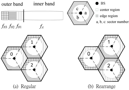
Figure 1.
Regular and rearranged frequency planning for a tri-sector cellular system.
2. Tri-Sector FFR-Based Frequency Partition
ICIC technique aims at minimizing CCI by efficiently coordinating channel allocation in adjacent cells. On top of network MIMO, this section introduces two FFR-based ICIC frequency reuse schemes as shown in Figure 1. The spectrum is divided into the inner frequency band and outer frequency band , where is further partitioned into three equal sub-bands (, and ) [12,15]. The inner and outer frequency bands are for CCUs’ and CEUs’ exclusive use, respectively. The differentiation between CEU and CCU can be made based on the received signal-to-interference-plus-noise ratio (SINR) at the user equipment [17]. All the CCUs within a cell share the sub-channels in inner frequency band . However, we serve a CEU either on a specific sub-channel of a sub-band or on an entire sub-band for SU- and MU-network MIMO, respectively. Specifically, the inner band adopts universal reuse factor with omni-directional antenna for CCUs; the outer bands uses frequency reuse factor of three for CEUs in each sector.
As mentioned in the previous section, we consider two frequency partitions (regular and rearranged) in Figure 1 [12]. Traditionally, the regular frequency planning in Figure 1a is the FFR-based frequency partition for a tri-sector cellular system, where the sectors of different cells with the same outer sub-band have the same main-beam direction. Accordingly, with regular frequency planning, the contiguous cell-edge areas of neighboring cells are assigned to different orthogonal outer sub-bands to avoid CCI as shown in Figure 1a. On the contrary, with rearranged frequency planning, the sectors of different cells with the same outer sub-band have different main-beam direction as shown in Figure 1b, where contiguous cell-edge areas of neighboring cells are with the same outer sub-bands.
In both SU- and MU-network MIMO, each CEU is served by a group of collaborative BSs. These BSs form a cooperative cell set (CCS) associated with that CEU. For convenience, let a BS sector denote the sector of cell . For example, consider a certain CEU located in the cell-edge area of sector for regular frequency planning in Figure 1a. For this CEU , we have the corresponding CCS , which use a particular sub-channel selected from outer sub-band to collectively serve the CEU . This is SU-network MIMO transmission. As in frequency-division multiple access (FDMA), SU-network MIMO allocates each CEU a unique sub-channel from an outer sub-band and thus the cooperative BSs in a CCS result in no multi-user interference. As for the rearranged one in Figure 1b, the collaborative BSs in CCS turn to together serve a group of their CEUs using the sub-band (i.e., MU-network MIMO), i.e., all CEUs in this group share the entire sub-band . As a result, the serious multi-user interference is inevitable. To control this, joint preprocessing among cooperative BSs is necessary in MU-network MIMO with rearranged frequency planning.
3. Signal Model
In this section, we present OFDMA-based signal models for CCU point-to-point transmission and 3-cell coordinated transmission, including MU- and SU-network MIMO. Consider a CCS as shown in Figure 1, where each cell employs 120° sectoring and is divided into cell-center and cell-edge regions. Users located in cell-center and cell-edge regions are referred to as CCUs and CEUs, respectively. We apply the traditional point-to-point and 3-cell coordinated transmission to CCUs and CEUs, respectively. Assume that each sector and each user are equipped with sector antennas and receiver antennas, respectively. The antenna pattern for each sector antenna in decibel is specified by [18]
where is the angle between the direction of interest and the main-beam of the antenna, is the 3-dB beamwidth in degree and is the maximum attenuation for the sidelobe.
The overall radio channel model at subcarrier of user with respect to BS is represented by
where denotes the small-scale Rayleigh fading, represents the shadowing effect and is the path loss. The cross-correlation model for the shadowing effect is given by
where is the difference of angle-of-arrival between two radio links observed at the receiver. The propagation loss model between a user and a BS is given by [19]
where represents the propagation constant, is the propagation distance in kilometer and denotes the path loss exponent. According to Shannon theorem, the achievable channel capacity is given by
where denotes bandwidth of the channel, represents the SINR. The parameter is the SINR gap with the target bit error rate (BER) [20]. In this paper, the target BER is given by .
3.1. MU-Network MIMO Signal Model
Consider a 3-cell coordinated MU-network MIMO as shown in Figure 1b, where 3 cooperative BSs together serve a group of their CEUs using the whole outer sub-band . Assume a proper cyclic-prefix length is appended to the inverse discrete Fourier transform (IDFT) sequence such that the inter-symbol interference can be ignored. After DFT, the signal reception at subcarrier by receiver antenna of CEU is:
where denotes the overall channel gain at subcarrier from transmitter antenna of BS to receiver antenna of CEU . Similarly, represents the pre-coded symbol transmitted from antenna of BS to CEU . The notation denotes the index set of subcarriers of the outer sub-band . is the received noise with single-sided power spectral density .
Let denote the index of the th subcarrier in for , where represents the cardinality of the set . We further represent the DFT sequence of (6) as a vector , which is given by the following matrix-vector form
where is a diagonal channel matrix with as its th diagonal element. Both and are vectors, whose th entry are and , respectively.
For later use, we define , which denotes the aggregate channel matrix observed at the receiver antenna of CEU from transmit antennas of BS . Similarly, the aggregate channel matrix observed at the antenna of CEU from all three cooperative BSs is given by
where represents the complex space. The aggregate signal vector sent to CEU from transmit antennas of BS can be represented as
To gain insight into how joint preprocessing works, we cascade all the received vectors of (7) to form a received vector, as shown below:
where is the aggregate channel matrix of user , is the aggregate signal vector sent for CEU from all 3 coordinated BSs, and is the aggregate received noise vector.
The aggregate signal vector associated with CEU results from jointly processing a data vector by all cooperative BSs, where is the number of data symbols sent to CEU in a network MIMO transmission. Specifically, the cooperative BSs jointly design a preprocessing matrix for the data vector , by which the signal vector is produced in the sense of mitigating the multi-user interference from other co-channel CEUs. In summary, the aggregate signal vector is produced according to
Define , which is the total number of CEU data symbols sent in a network MIMO transmission. Substituting (11) into (10), we have a more concise expression for the aggregate received DFT vector of (10) as follows:
where the aggregate data vector is
and is the completely aggregate preprocessing matrix given by
3.2. CCU Point-to-Point and SU-Network MIMO Signal Models
We have presented the signal model for CEUs in MU-network MIMO. In this sub-section, we first present the CCU point-to-point signal model. For CCU , the DFT signal at subcarrier received from the serving BS by its receiver antenna is
There is no intra-cell interference because each CCU is assigned a different sub-channel from the inner band . Here, the index set of subcarriers is associated with a particular sub-channel selected from the inner band .
As for the CEUs in SU-network MIMO, consider a 3-cell coordinated network MIMO as shown in Figure 1a, where each CEU is together served by 3 cooperative BSs using a different sub-channel from an outer sub-band. For instance, a CEU located at cell-edge region of sector 0(a) would be collectively served by the 3 cooperative BSs using a sub-channel selected from outer sub-band . Thus, after DFT, the signal reception at subcarrier by receiver antenna of CEU can be expressed as
where the index set of subcarriers is associated with a particular sub-channel selected from an outer band fBi.
4. Joint Preprocessing Techniques for MU-Network MIMO
As mentioned previously, the serious multi-user interference is inevitable in MU-network MIMO. To control this, joint preprocessing among cooperative BSs is necessary. With per-sector antenna power constraint, we derive various joint preprocessing schemes for OFDMA-based MU-network MIMO. They include MU joint time-division multiple access (MU-JTDMA), MU joint zero-forcing (MU-JZF), and MU joint minimum mean-square error (MU-JMMSE). Both MU-JZF and MU-JMMSE are superposition-coding schemes and MU-JTDMA is an orthogonal one.
Recall that the signal vector sent to CEU from all 3 coordinated BSs is the aggregate signal vector . Accordingly, the preprocessing matrix in (11) can be decomposed as
where BS uses sub-matrix to pre-code data vector , i.e., . Then the total power required by BS to serve all the CEUs is given by
where is the statistical expectation operator, denotes the trace of a square matrix, the superscript denotes Hermitian transpose and is the covariance matrix of with zero-mean uncorrelated data symbols.
4.1. MU-JTDMA
In MU-JTDMA, the collaborative BSs together serve each of their CEUs at a different time slot. Thus, it is free from multi-user interference at the cost of spectral efficiency. In [21], it was shown that the receiver side (say CEU ) equivalently observes a equivalent parallel channels:
where is the th non-zero singular value of aggregate channel matrix and denotes the received noise.
4.2. MU-JZF
The MU-JZF scheme enables complete suppression of interference, but it demands higher transmitter power for the jointly pre-coding process. To derive the preprocessing matrix, we stack up the received vector in (12) to form
where , and are the aggregate channel matrix, aggregate preprocessing matrix and aggregate noise vector for the entire network MIMO, respectively. Since the aggregate channel matrix is a random matrix, it has full rank with probability one. With ZF criterion, the square matrix product in (20) must be an identity matrix. This requires that the aggregate channel matrix have a full row rank of [22]. As a result, this leads to the inequality , which is usage constraint of MU-JZF. To satisfy this constraint, each per-CEU channel matrix of must be full row rank of and (the number of data symbols sent to CEU ) will be equal to .
Then the aggregate preprocessing matrix in (20) is the following pseudo-inverse of aggregate channel matrix :
Applying (21) to (20), the received signal vector of (12) becomes the equivalent parallel channels:
4.3. MU-JMMSE
The MU-JZF completely eliminates the multi-user interference at the cost of demanding higher transmitter power. The MU-JMMSE makes an acceptable compromise between interference suppression and transmitter power efficiency. Based on the MMSE criterion [21,23], the aggregate preprocessing matrix is
where is the transmission power for each data symbol.
5. Transmission Power Management
As mentioned earlier, each of BSs in a CCS together serves its own users and the CEUs of other collaborative BSs under a power constraint. Therefore, it is necessary to develop a method of distributing transmitter power among intra-cell CCUs, intra-cell CEUs, and inter-cell CEUs. To the best of our knowledge, however, there has been no literature dealing with this issue. The purpose of power management is to achieve a uniform capacity regardless of user position. Because of the cooperation with the neighboring BSs, the design of power management may involve the information exchange among the cooperative-based stations. Due to the time-variant characteristics of channel, this continuing need for information exchange will consume a lot of radio resources. In the absence of information exchange, our method of power management for MU-network MIMO cellular systems only needs the number of different types of users to realize an independent power adjustment among BSs.
Let , and denote the sub-channel power allocated for an intra-cell CCU, intra-cell CEU, and inter-cell CEU, respectively. Let denote a sub-channel baseline power and represent the maximum transmission power constraint in a sector antenna. In our method, a CCU and a CEU are respectively allotted the initial power and , where the power coefficient , i.e., we initially set and .
The power management is conducted in a per-sector basis. Let , and denote the number of intra-cell CCUs, intra-cell CEUs, and the inter-cell CEUs served by a particular sector antenna, respectively. Thus, the total power requirement is , where the power required to serve other cells’ CEUs is . In the subsequent sub-sections, we present transmission power management for SU- and MU-network MIMO, respectively.
5.1. Power Management for SU-Network MIMO
For a specific CCS, define to be the power ratio consumed by inter-cells’ CEUs, i.e., we partition the total transmitter power into two parts: power for intra-cell users and power for inter-cells’ CEUs (). Accordingly, we can use the power ratio to limit the maximum power dispensed to inter-cells CEUs. Therefore, the power consumption is limited within . In a per-sector antenna basis, the procedure of power management is presented as follows.
- (a)
- Initialize the power allocation to each of CCUs and CEUs by and , respectively.
- (b)
- Calculate the amount of power consumed by the other cells’ CEUs (i.e., ). If , then reduce the power allocation for each inter-cell CEU by a factor of such that the amount of power consumption by the other cells’ CEUs equals the power constraint , where ; elsewise .
- (c)
- Next calculate the total transmission power for intra-cell users (i.e., ). If , then reduce the initial power by a factor of such that equals the upper bound power , where ; elsewise .
- (d)
- Finally, we achieve , and .
In summary, the method consists of a CEU power coefficient and two power reduction factors ( and ). The coefficient is used to determine the power proportion between a CCU and a CEU. The power allotted to other cells’ CEUs can be restricted by power reduction factor together with the power ratio . As for the power reduction factor , it prohibits a power requirement from exceeding the corresponding power constraint . To best use the transmitter power, we initially assume that the baseline power is equal to . Thus, the two power portions and can be fully used.
5.2. Power Management for MU-Network MIMO
Unlike SU-network MIMO, each of CEUs in MU-network MIMO shares the entire sub-band instead, as shown in Figure 1b. This yields serious multi-user interference and thus joint preprocessing among cooperative BSs becomes necessary, as discussed in Section 4. Since the preprocessing matrices are jointly designed for all the CEUs, there is no distinction between intra-cell and inter-cell CEUs . Thus, there is no need for for power management in MU-network MIMO. Initially the power for each intra-cell CCU is . The total power requirement for cooperative BS to serve the CEUs is as shown in (18). We define the average preprocessing power for a CEU as . As in SU-network MIMO, the CEU power is . However, the CEU power depends on the average preprocessing power , which is variable because of the time-variant channel. Thus, we further let the CEU power be , where is determined such that . Therefore, we achieve .
For each sector antenna, the procedure of power management is as follows.
- (a)
- Initialize the power allocation to each of CCUs by .
- (b)
- Calculate the average preprocessing power according to (18). Then set the CEU power , where .
- (c)
- Next, calculate the total power requirement . If , then reduce the baseline power by a factor of such that the value of equals the power constraint , where ; elsewise .
- (d)
- Finally, we achieve and .
In summary, the method consists of a CEU power coefficient and a power reduction factor . We adaptively adjust the value of such that . The power reduction factor is used to make sure that the total power requirement does not exceed the power constraint .
6. Simulation Results
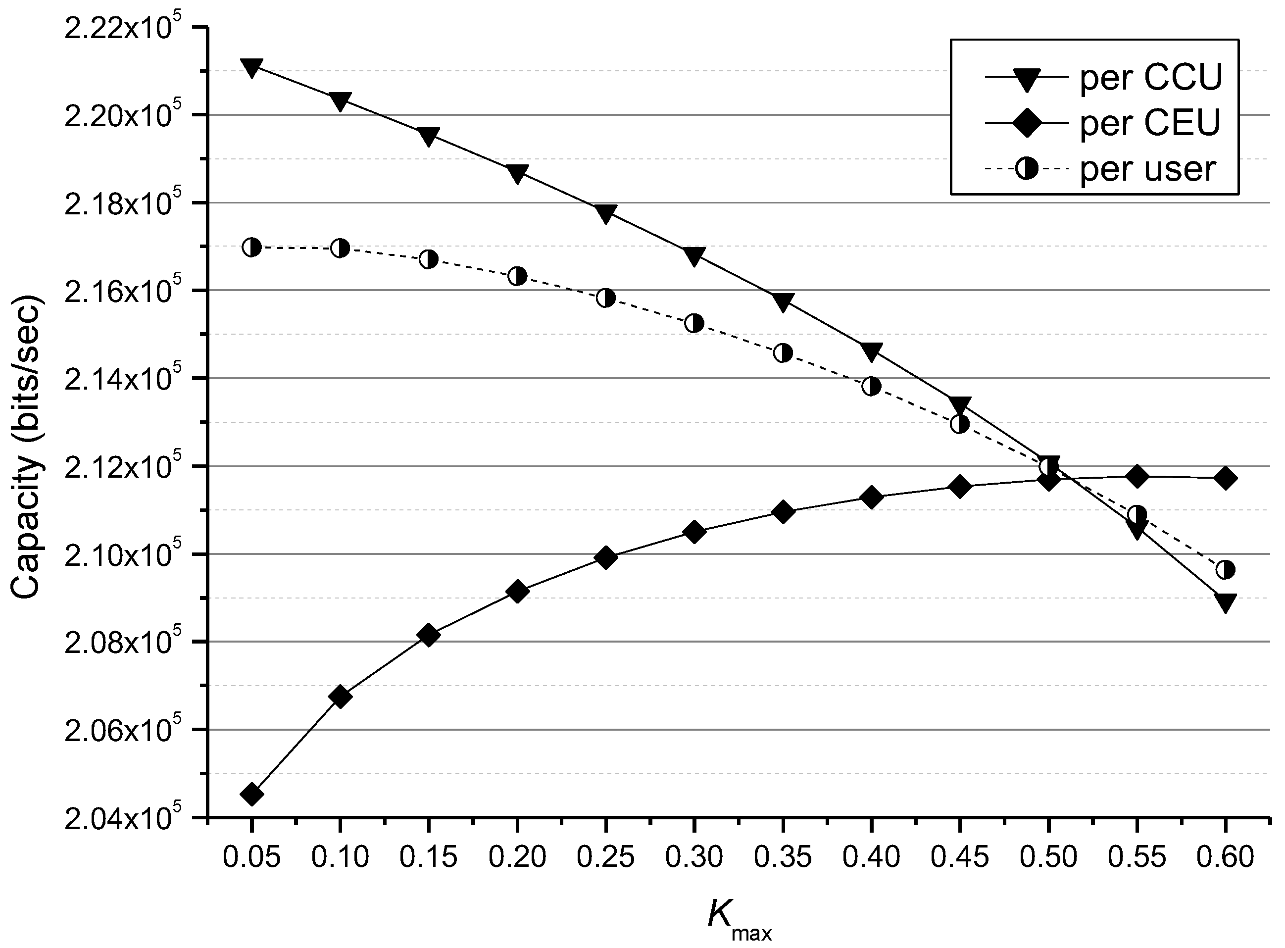
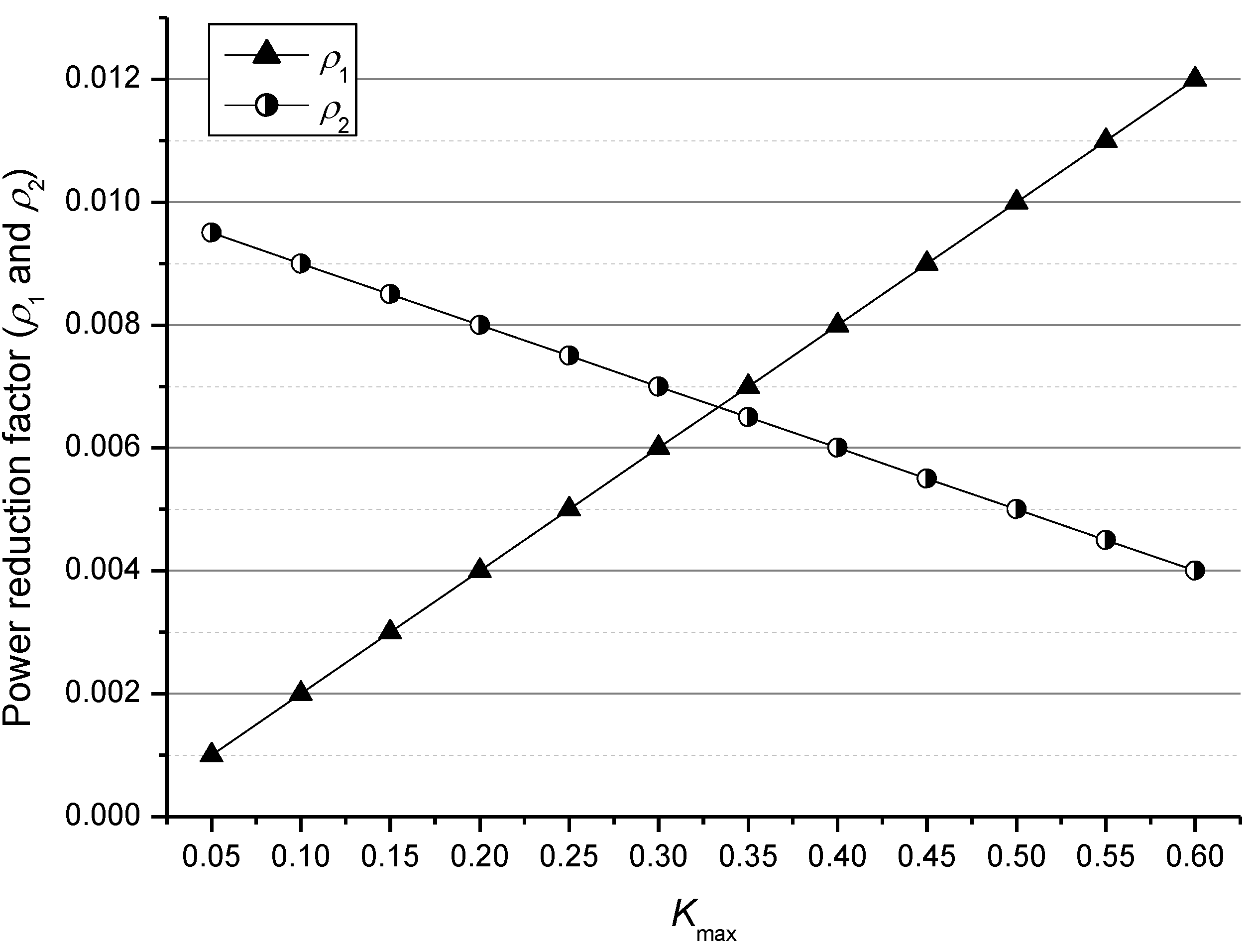
This section presents performance comparison between SU and MU-network MIMO with the power management methods. Unless otherwise stated, the cell radius and cell-center radius are 1000 m and 787.55 m, respectively. Accordingly, within a sector, the ratio of cell-center area to cell-edge area is 3 to 1. Assume users are uniformly distributed in each cell. Thus, we set the ratio of sub-channel number between inner band and outer band to be 3 to 1 as well. To this end, we assume the total number of OFDMA sub-channels is 60 such that the numbers of sub-channels in and are integers 45 and 15, respectively. Therefore, each outer sub-band consists of 5 OFDMA sub-channels. As a result, for SU-network MIMO, there are at most five active CEUs in each sector (hard CEU capacity). As for MU-network MIMO, joint preprocessing makes it possible that more than five CEUs in each sector can be served at the same time (soft CEU capacity). Assume there are 12 subcarriers in a sub-channel and the sub-channel bandwidth is 138.8 KHz. The maximum power constraint is 46.523 dBm [2]. The propagation constant and path loss exponent are and 3, respectively [20]. The standard deviation of log-normal shadowing is 12 dB. Unless otherwise stated, there are 15 CCUs and 5 CEUs uniformly distributed in each sector, each sector is equipped with five transmission antennas and the power coefficient is one . As for users, each of them is equipped with a single receiver antenna . In terms of different values of , Figure 2 shows the capacity comparison for SU-network MIMO and Figure 3 presents its corresponding curves of power reduction factors. In Figure 2, we find that smaller yields better per-user (average) capacity than larger . However, smaller results in bigger capacity gap between CCU and CEU than larger . Thus, through continuing enlarging the value of , the capacity gap can be reduced, but it is at the cost of decreasing the average capacity. For example, in Figure 2, an equal CCU and CEU capacity (zero capacity gap) occurs at about , i.e., a uniform capacity is achieved regardless of user position; however, it obviously reduces the average capacity. Figure 3 shows that while the value of is increasing, the power factor is increasing as well. This is because a larger value the means that more transmitter power is allocated to the inter-cell CEUs. Accordingly, the power factor associated with intra-cell users is decreasing while the value of is increasing.
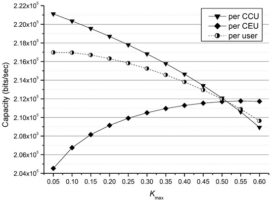
Figure 2.
Capacity comparison for SU-network MIMO in terms of different values of Kmax.

Figure 3.
Curves of power reduction factors associated with Figure 2.
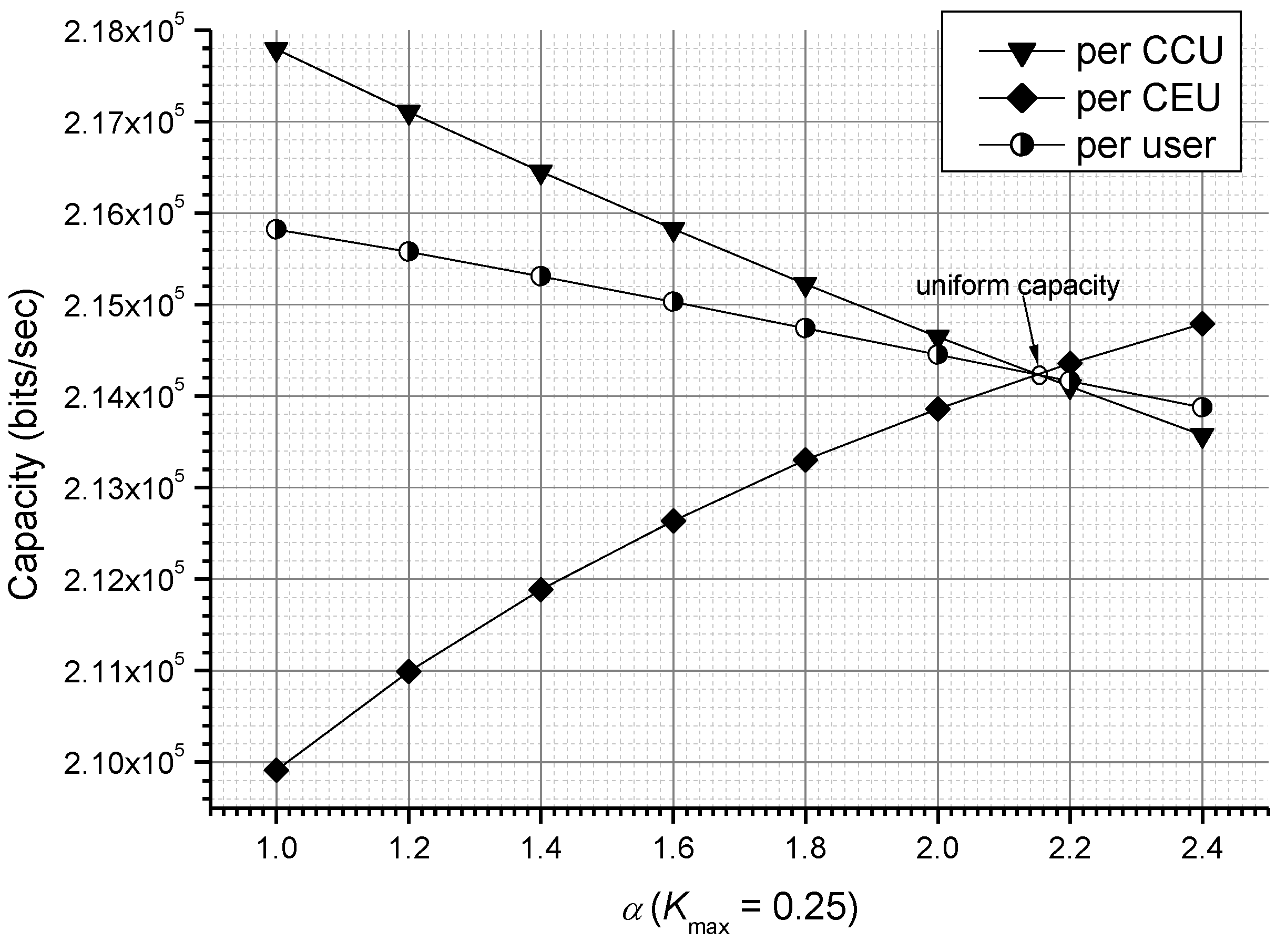
As a function of power coefficient , Figure 4 shows the capacity comparison for SU-network MIMO with a small (say ). Please note that the CEU power is given by . Thus, we can raise the CEU power by increasing the value of . It is found that increasing the value of can actually diminish the capacity gap between CCU and CEU, and a uniform capacity is achieved at . However, the average (per-user) capacity is also slowly decreasing at the same time, while the capacity gap is decreasing. In Figure 5, we present the capacity comparison as a function of for a large (say ). It is shown that the uniform capacity occurs at a smaller , , as compared with associated with the smaller in Figure 4. By making a comparison between Figure 4 and Figure 5, it is found that the per-user (average) capacity with smaller is always better than that with larger , although it yields larger capacity gap than that of larger . Nevertheless, while achieving uniform capacity (zero capacity gap), the smaller still yields better average capacity (about bits/sec) than that with the larger (about bits/sec). Therefore, with , SU-network MIMO offers more bits per second than that with . In conclusion, with uniform capacity, smaller can generally provide the SU-network MIMO with larger average capacity.
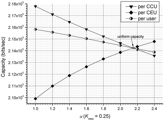
Figure 4.
Capacity comparison as a function of for a small in SU-network MIMO.

Figure 5.
Capacity comparison as a function of for a large in SU-network MIMO.
Uniform capacity makes sure that users have uniform data rate regardless of their position. According to the previous results, we found that uniform data rate comes at the price of reducing the average capacity. Studies on wireless usage show that more than 50% of all voice calls and more than 70% of data traffic originate from indoors (i.e., immobile conditions) [24]. As a result, the uniform capacity is only important for the small part of truly mobile users. For example, as a mobile user with SU-network MIMO moves from cell center to cell border, the cell-edge capacity will drop a small percentage as compared with cell-center capacity, and thus the user may be deficient in capacity. Thus, uniform data rate is essential for this scenario.
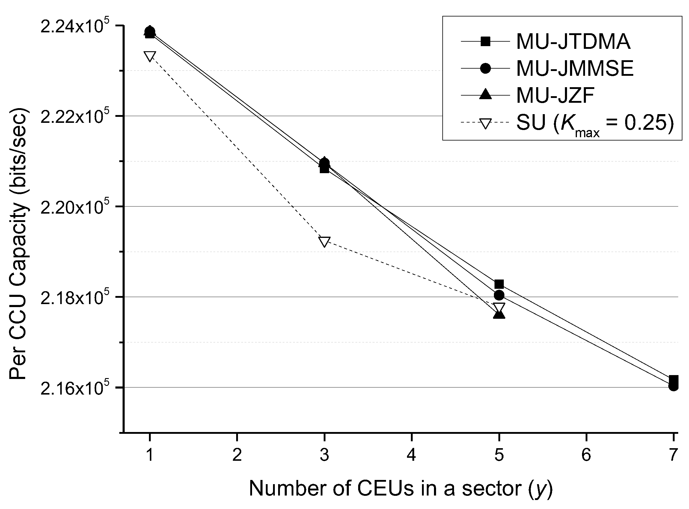
Now we turn our attention to the MU-network MIMO and in the meantime, make comparison with SU-network MIMO. In terms of the number of per-sector CEUs (), Figure 6 presents the per-CCU capacity comparison for three MU-network MIMO schemes and the SU-network MIMO. Recall that three cooperative BSs in a CCS collectively serve a group of CEUs using a whole out sub-band. Thus, we have for MU-network MIMO. In MU-network MIMO, both MU-JMMSE, and MU-JTDMA have soft CEU capacity, but MU-JZF does not, because it is subject to the usage constraint as shown in Section 4.2. In general, it is found that MU-network MIMO is better than SU-network MIMO in CCU capacity, except for MU-JZF at , whose CCU capacity is slightly less than SU-network MIMO. Figure 7 gives the per-CEU capacity comparison. Except for the orthogonal scheme (MU-JTDMA), it is found that the superposition-coding schemes (MU-JMMSE and MU-JZF) have obvious CEU capacity improvement over the SU-network MIMO [25]. In addition, since there are just 5 sub-channels in an outer frequency sub-band, the SU-network MIMO only can serve up to 5 CEUs per sector. By contrast, the MU-network MIMO has a soft capacity for CEUs, except for MU-JZF because it is subject to the usage constraint . For example, as increasing two additional CEUs from 5 CEUs to 7 CEUs in each sector, we calculate that the MU-JMMSE only drop about 0.9% and 15.2% for per-CCU and per-CEU capacity, as shown in Figure 6 and Figure 7, respectively.
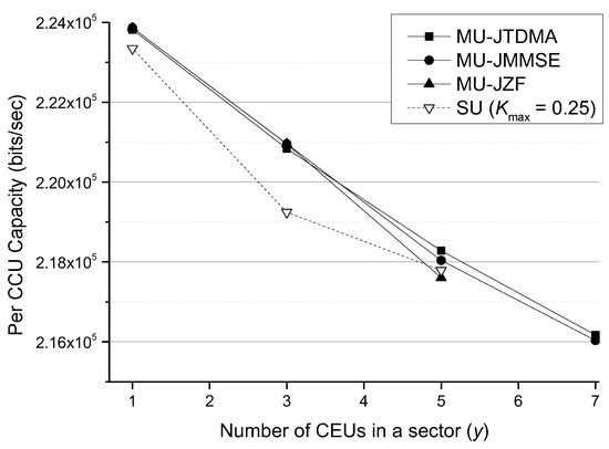
Figure 6.
Per-CCU capacity comparison between the MU and SU-network MIMO.
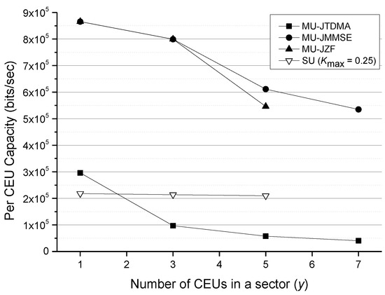
Figure 7.
Per-CEU capacity comparison between the MU and SU-network MIMO.
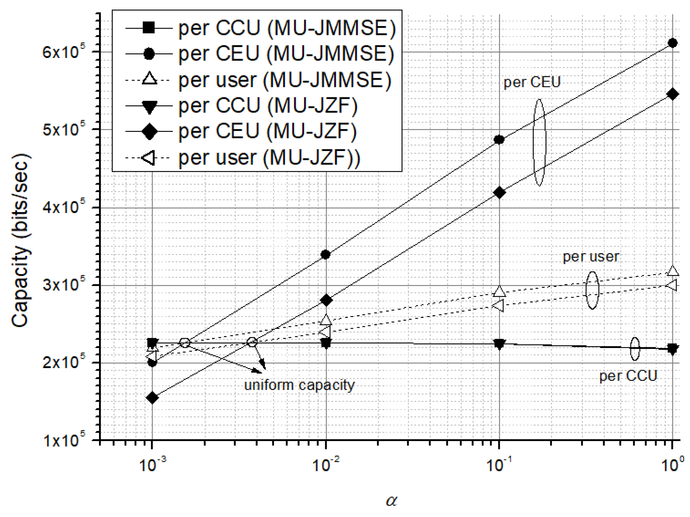
Figure 8 shows the capacity comparison for both superposition-coding schemes (MU-JMMSE and MU-JZF) as a function of . It is found that the per-CEU capacity is much better than the per-CCU capacity (at ) because of joint preprocessing. By contrast, for SU-network MIMO with , its per-CEU capacity is still distinctly worse than the per-CCU capacity, as shown previously in Figure 4 and Figure 5. This means that the joint preprocessing (superposition coding) offers great preprocessing gain that benefits per-CEU and per-user (average) capacities. Recall that , where is the CCU power. Due to the excellent preprocessing gain, the MU-network MIMO can use extremely small value of (i.e., very small CEU power) to achieve uniform data rate, say and for MU-JMMSE and MU-JZF, respectively. This is opposite to SU-network MIMO. Moreover, it is found that MU-JMMSE is better than MU-JZF. This is because MU-JZF completely eliminates the CCI at the cost of demanding higher transmitter power. However, MU-JMMSE makes an acceptable compromise between interference suppression and transmitter power efficiency.
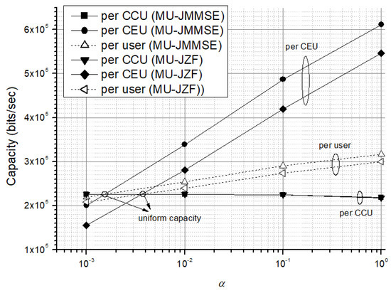
Figure 8.
Capacity comparison for joint preprocessing schemes in MU-network MIMO as a function of .
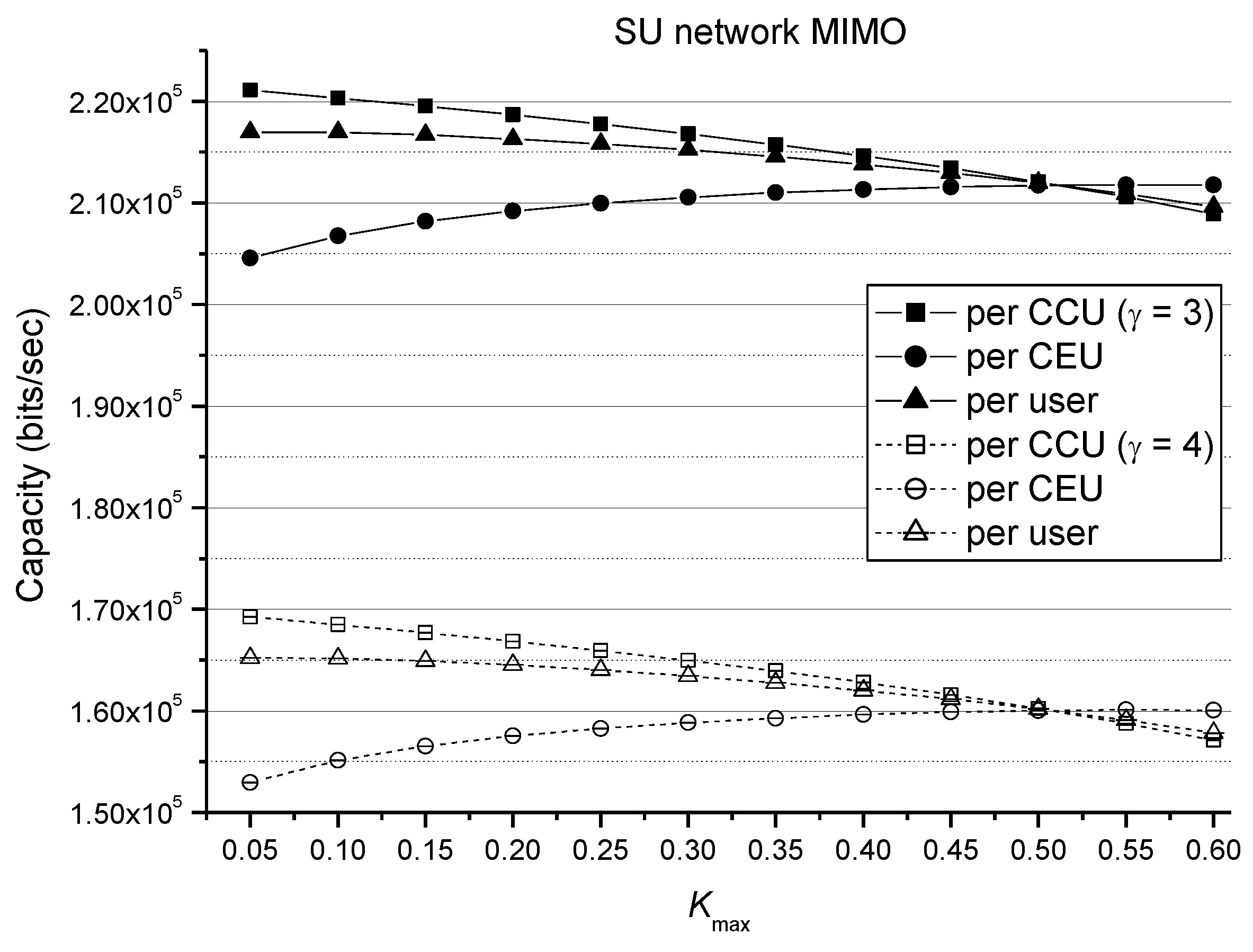
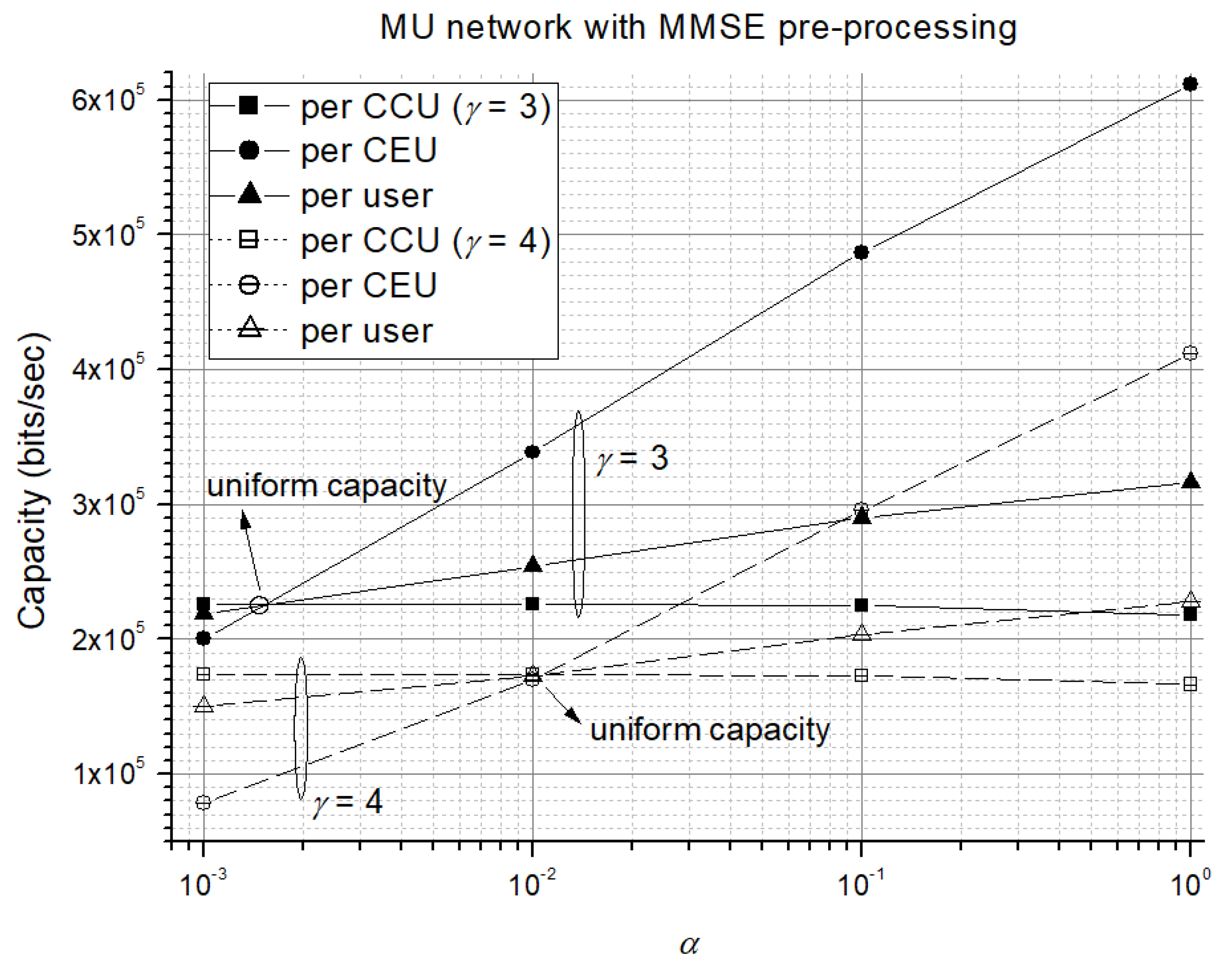
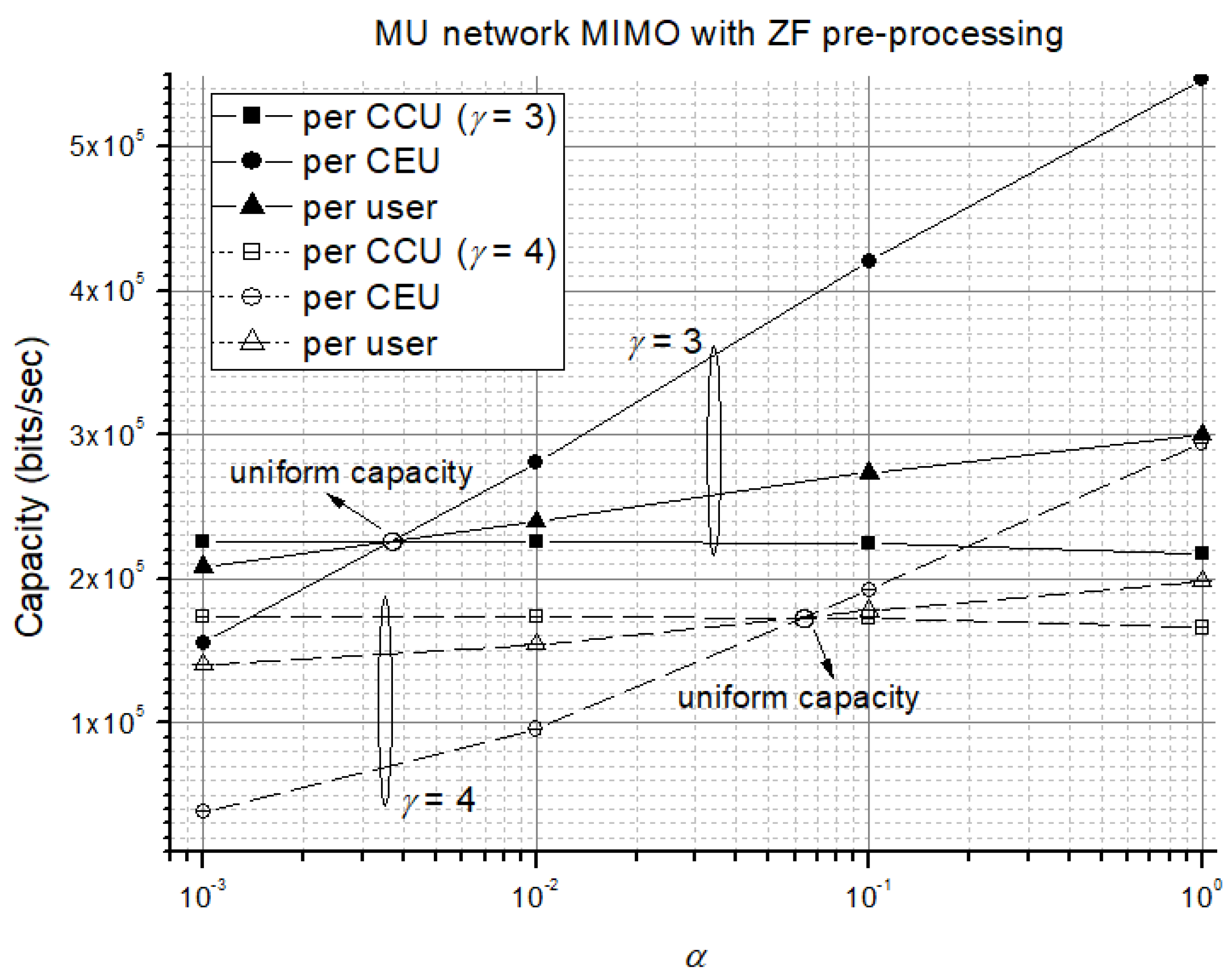
The numerical results above are obtained under the path loss exponent of 3. Changing the value of to a typical value of 4 does not influence the previous numerical results. For example, Figure 9 shows the same observations in SU-network MIMO for both path loss exponents (), i.e., smaller yields better per-user (average) capacity than larger . However, smaller produces bigger capacity gap between CCU and CEU than larger . Likewise, in MU-network MIMO, the observed phenomena are also the same for different values of path loss exponent. Figure 10 and Figure 11 show the capacity comparison between different values of path loss exponent with MMSE and ZF joint preprocessing, respectively. It is found that the per-CEU capacity is much better than the per-CCU capacity at because of taking advantage of joint preprocessing. It is worth mentioning that, however, although the path loss increases with a larger path loss exponent , we need to allocate more power to CEUs by increasing the value of to achieve a uniform capacity as shown in Figure 10 and Figure 11.

Figure 9.
Capacity comparison between different values of path loss exponent for SU-network MIMO.
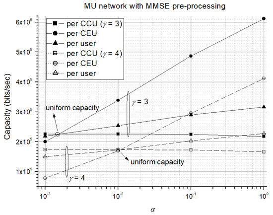
Figure 10.
Capacity comparison between different values of path loss exponent for MU-network MIMO with MMSE joint preprocessing.
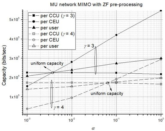
Figure 11.
Capacity comparison between different values of path loss exponent for MU-network MIMO with ZF joint preprocessing.
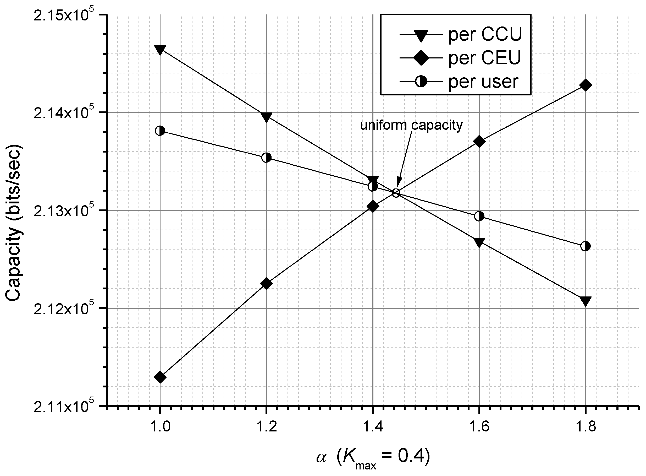
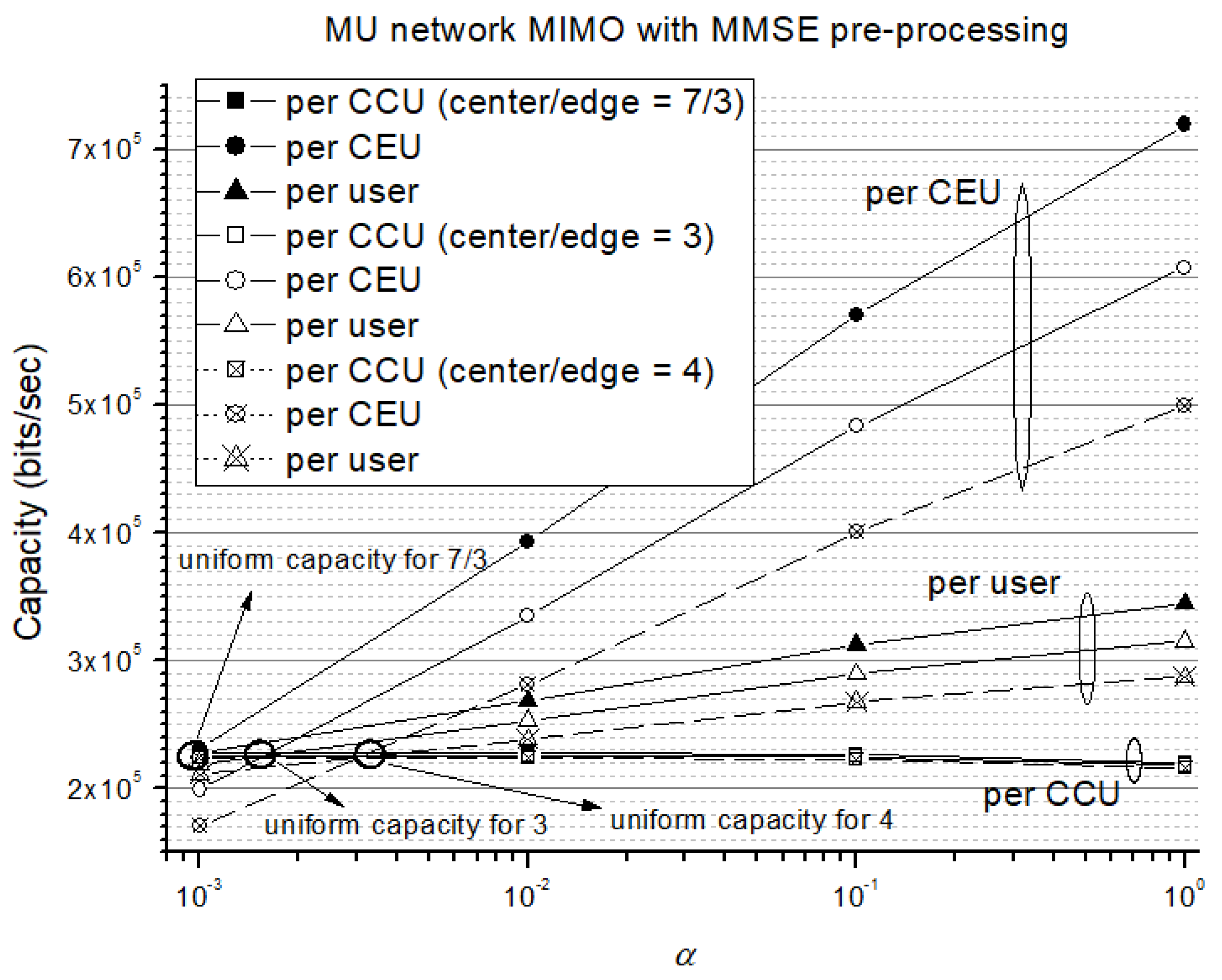
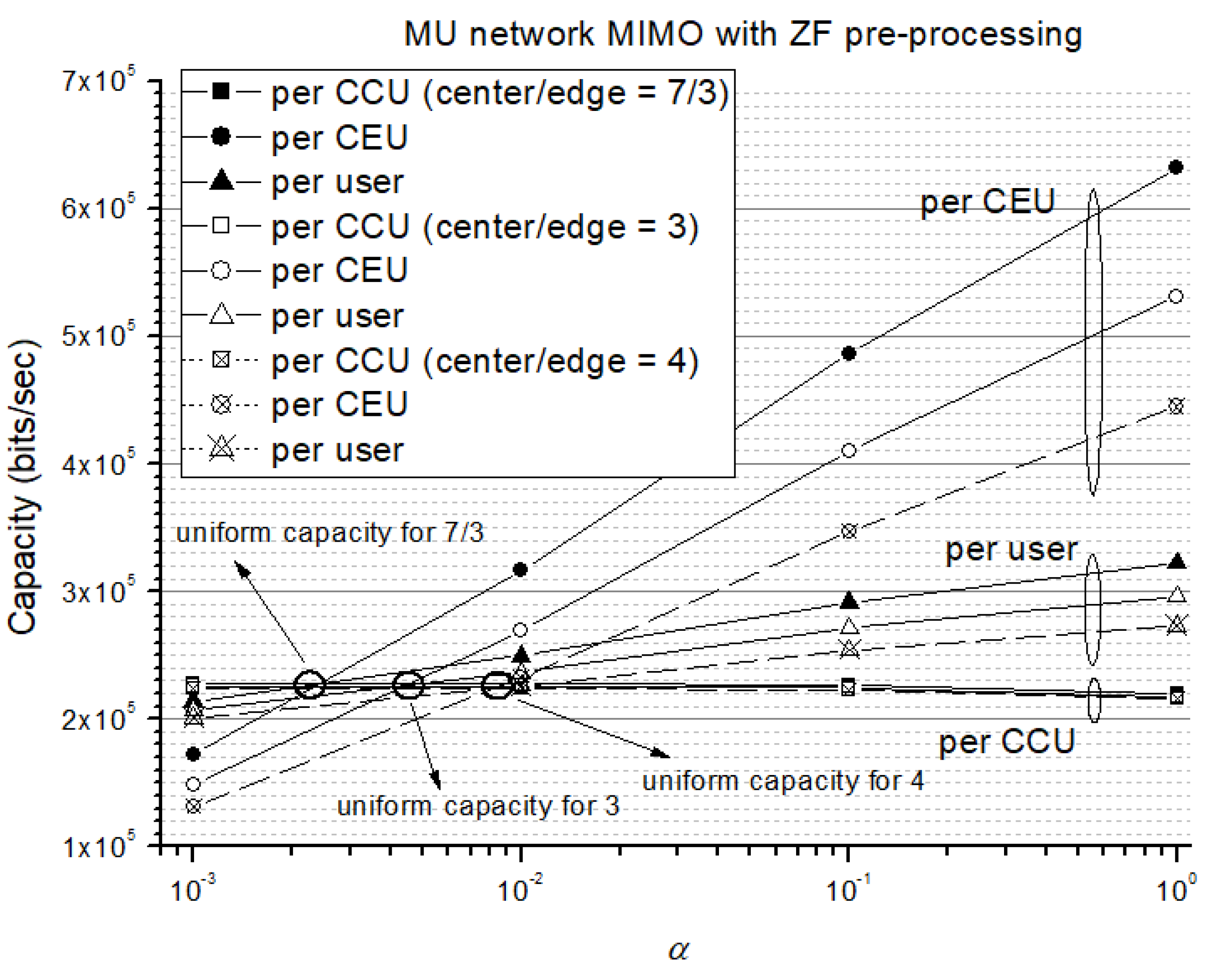
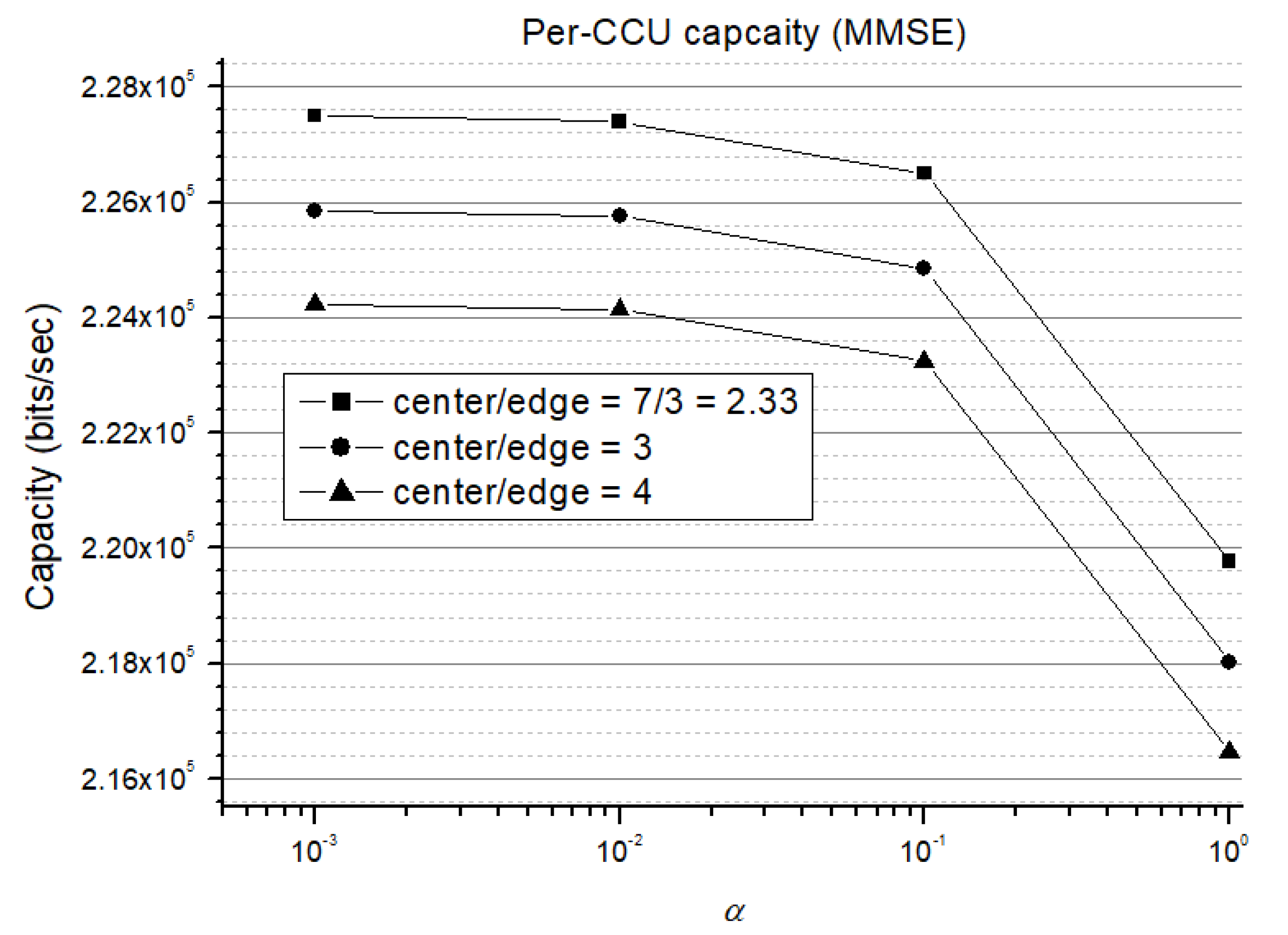
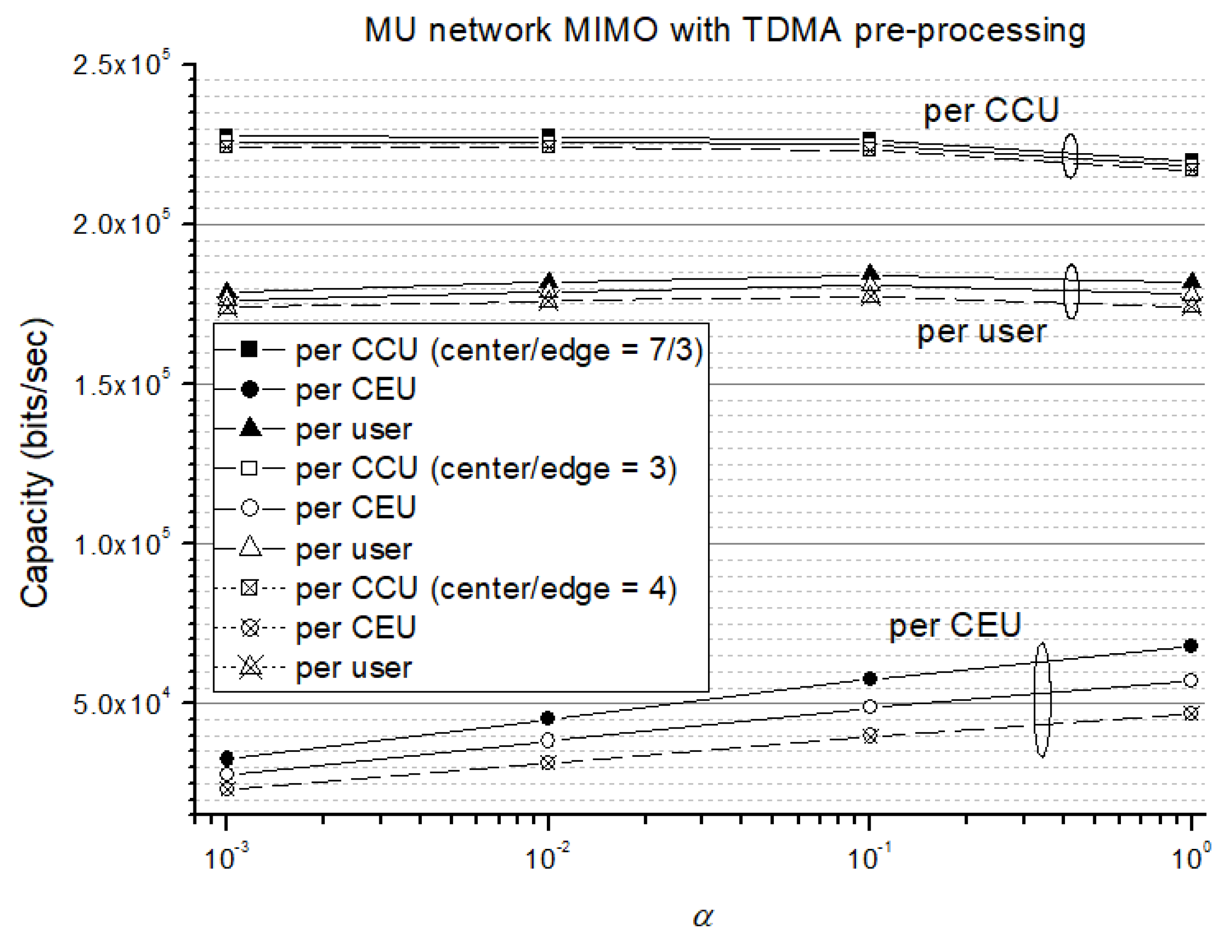
Next, we show how the different ratios between cell-center and cell-edge area influence the result. Figure 12 and Figure 13 are numerical results for the superposition-coding MU-MMSE and MU-ZF joint preprocessing schemes, respectively. Because the variation of CCU capacity is much less obvious than that of CEU capacity, we give a separate illustration for CEU capacity in Figure 14, where only the MMSE CCU capacity is shown because both MMSE and ZF are similar. The result of the orthogonal MU-TDMA joint preprocessing scheme is given in Figure 15. Finally, Figure 16 shows the result for the SU-network MIMO. With superposition-coding MU-MMSE and MU-ZF schemes, Figure 12 and Figure 13 indicate that reducing the ratio (i.e., increasing the edge area, but decreasing the center area) significantly benefits the CEU capacity. For example, this can be found from the decrease in the value of α to achieve uniform data rate as shown in Table 1. As for the CCU, while cell-center area is reduced, the interference from neighboring cells is decreased and thus there is also a slight increase in CCU capacity as shown in Figure 14. In Figure 15, the result of the orthogonal MU-TDMA joint preprocessing scheme is similar to the superposition-coding schemes, i.e., increasing the cell-edge area benefits the capacity for either CEU or CCU capacity. The same observations are also true for SU-network MIMO in Figure 16, where we just show two different area ratios for clarity of illustration. It also shows that decreasing the center area significantly benefits the CEU capacity and improves the CCU capacity slightly. Overall, the system capacity increases due to enlarging the cell-edge area, which directly increases the proportion of downlink multi-cell cooperation (network MIMO) transmission. With network MIMO, multiple geographically separated base stations cooperatively serve their CEUs using their antennas, acting together as a network of distributed antenna array. In fact, this network architecture not only can effectively mitigate the serious co-channel interference but also provide diversity transmission. However, it is worth mentioning that the disadvantages of cooperative transmission require additional overhead for information exchange among cooperative BSs.
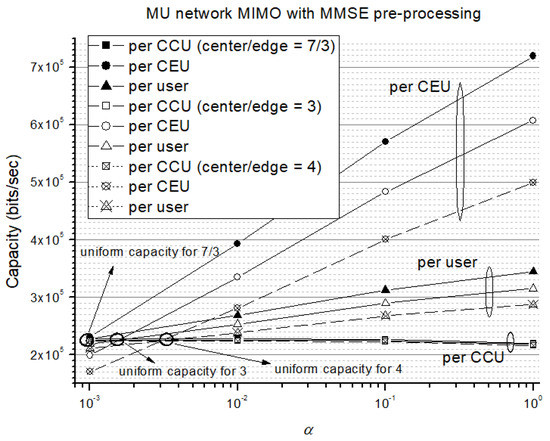
Figure 12.
Capacity comparison between different values of center-edge area ratio for MU-network MIMO with MMSE joint preprocessing.
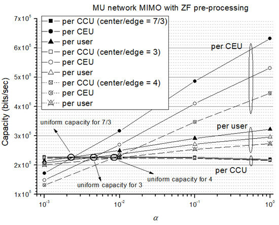
Figure 13.
Capacity comparison between different values of center-edge area ratio for MU-network MIMO with ZF joint preprocessing.
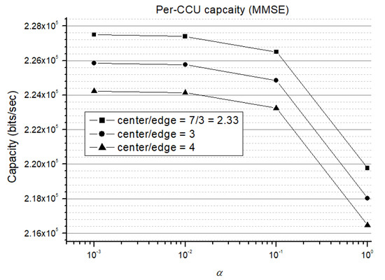
Figure 14.
Per-CCU Capacity comparison between different values of center-edge area ratio for MU-network MIMO with MMSE joint preprocessing.
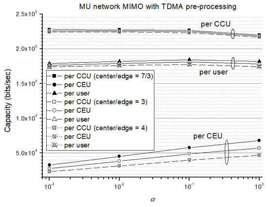
Figure 15.
Capacity comparison between different values of center-edge area ratio for MU-network MIMO with TDMA orthogonal joint preprocessing.
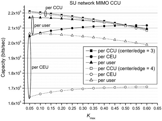
Figure 16.
Capacity comparison between different values of center-edge area ratio for SU-network MIMO.

Table 1.
The distribution of the value of .
7. Conclusions
In this paper, we have investigated both the SU and MU-network MIMO based on FFR-based ICIC, together with their power management methods. Two considered FFR-based ICIC are regular and rearranged frequency partitions, which are associated with SU and MU-network MIMO, respectively. With regular partition, the SU-network MIMO can avoid the multi-user interference, but it just has a hard CEU capacity. As for rearrange partition, MU-network MIMO needs joint preprocessing among cooperative BSs to deal with the serious multi-user interference. However, it can provide soft capacity for CEUs. To this end, we have derived three joint preprocessing schemes, including two superposition-coding schemes (MU-JZF and MU_JMMSE) and an orthogonal one (MU-JTDMA).
Uniform capacity makes sure that users can acquire uniform data rate regardless of their position. To achieve uniform data rate for SU-network MIMO, we can adjust either the power coefficient or power ratio Kmax. For MU-network MIMO with unit power coefficient, because of the excellent preprocessing gain, the superposition-coding schemes yield much better CEU capacity and slightly better CCU capacity as compared with the SU-network MIMO. As a result, the MU-network MIMO can allocate very small power to CEUs by greatly reducing the value of power coefficient to achieve a uniform data rate.
Author Contributions
Conceptualization, J.-S.S.; methodology, J.-S.S. and K.-M.H.; software, J.-S.S. and K.-M.H.; validation, J.-S.S. and K.-M.H.; formal analysis, J.-S.S.; investigation, J.-S.S.; resources, J.-S.S. and K.-M.H.; data curation, J.-S.S. and K.-M.H.; writing—original draft preparation, J.-S.S. and K.-M.H.; writing—review and editing, J.-S.S.; visualization, J.-S.S. and K.-M.H.; supervision, J.-S.S.; project administration, J.-S.S. All authors have read and agreed to the published version of the manuscript.
Funding
This research received no external funding.
Data Availability Statement
The source codes of this studies are available at the following link: https://drive.google.com/drive/folders/1LvBDXByQIXKVKEInCjD8H8x9t2aXitJJ?usp=sharing (accessed on 31 October 2021).
Conflicts of Interest
The authors declare no conflict of interest.
References
- Chang, S.; Kim, S.; Choi, J.P. The Optimal Distance Threshold for Fractional Frequency Reuse in Size-Scalable Networks. IEEE Trans. Aerosp. Electron. Syst. 2020, 56, 527–546. [Google Scholar] [CrossRef]
- IEEE. Standard 802.16. Part 16: Air interface for fixed and mobile broadband wireless access systems–DRAFT amendment to IEEE standard for local and metropolitan area networks-advanced air interface, IEEE P802.16m/D4. Febuary 2010. Available online: https://standards.ieee.org/standard/802_16h-2010.html (accessed on 31 October 2021).
- Clark, M.V.; Erceg, V.; Greenstein, L.J. Reuse Efficiency in Urban Microcellular Networks. IEEE Trans. Veh. Technol. 1997, 46, 279–288. [Google Scholar] [CrossRef]
- Wang, J.; Wang, L.; Wu, Q.; Yang, P.; Xu, Y.; Wang, J. Less Is More: Creating Spectrum Reuse Opportunities via Power Control for OFDMA Femtocell Networks. IEEE Syst. J. 2016, 10, 1470–1481. [Google Scholar] [CrossRef]
- Hossain, M.S.; Becvar, Z. Soft Frequency Reuse with Allocation of Resource Plans Based on Machine Learning in the Networks with Flying Base Stations. IEEE Access 2021, 9, 104887–104903. [Google Scholar] [CrossRef]
- Ali, M.S.; Hossain, E.; Kim, D.I. LTE/LTE-A Random Access for Massive Machine-Type Communications in Smart Cities. IEEE Commun. Mag. 2017, 55, 76–83. [Google Scholar] [CrossRef] [Green Version]
- Soret, B.; Domenico, A.D.; Bazzi, S.N.; Mahmood, H.; Pedersen, K.I. Interference Coordination for 5G New Radio. IEEE Wirel. Commun. 2018, 25, 131–137. [Google Scholar] [CrossRef] [Green Version]
- Hamza, A.S.; Khalifa, S.S.; Hamza, H.S.; Elsayed, K. A Survey on Inter-Cell Interference Coordination Techniques in OFDMA-Based Cellular Networks. IEEE Commun. Surv. Tutor. 2013, 15, 1642–1670. [Google Scholar] [CrossRef]
- Kumar, S.; Kalyani, S.; Giridhar, K. Impact of Sub-Band Correlation on SFR and Comparison of FFR and SFR. IEEE Wirel. Commun. 2016, 15, 5156–5166. [Google Scholar] [CrossRef]
- Elayoubi, S.E.; Ben Haddada, O.; Fourestie, B. Performance Evaluation of Frequency Planning Schemes in OFDMA-based Networks. IEEE Trans. Wirel. Commun. 2008, 7, 1623–1633. [Google Scholar] [CrossRef]
- Ghosh, J.; Jayakody, D.N.K. An Analytical View of ASE for Multicell OFDMA Networks Based on Frequency-Reuse Scheme. IEEE Syst. J. 2020, 14, 645–648. [Google Scholar] [CrossRef]
- Wang, L.C.; Yeh, C.J. 3-Cell Network MIMO Architectures with Sectorization And Fractional Frequency Reuse. IEEE J. Sel. Areas Commun. 2011, 29, 1185–1199. [Google Scholar] [CrossRef]
- Lei, H.; Zhang, L.; Zhang, X.; Yang, D. A Novel Multi-Cell OFDMA System Structure Using Fractional Frequency Reuse. In Proceedings of the 2007 IEEE 18th International Symposium on Personal, Indoor and Mobile Radio Communications, Athens, Greece, 3–7 September 2007; pp. 1–5. [Google Scholar]
- Chiu, C.S.; Huang, C.C. Combined Partial Reuse and Soft Handover in OFDMA Downlink Transmission. In Proceedings of the VTC Spring 2008—IEEE Vehicular Technology Conference, Singapore, 11–14 May 2008; pp. 1707–1711. [Google Scholar]
- Sheu, J.S.; Lyu, S.H.; Lyu, S.J. Cell Sectorization and Power Management for Inter-Cell Interference Coordination in OFDMA-based Network MIMO Systems. In Proceedings of the 2014 IEEE Wireless Communications and Networking Conference (WCNC), Istanbul, Turkey, 6–9 April 2014; pp. 638–1642. [Google Scholar]
- Khan, F. LTE for 4G Mobile Broadband: Air Interface Technologies and Performance, 1st ed.; Cambridge University Press: Cambridge, UK, 2009. [Google Scholar]
- R1-090613: ‘Discussions on CoMP SU-MIMO’, Samsung, 3GPP TSG RAN WG1 Meeting #56. February 2009. Available online: https://www.3gpp.org/DynaReport/TDocExMtg--R1-56--27291.htm (accessed on 31 October 2021).
- R1-091983: ‘Way forward for Beamforming Antenna Gain Pattern’, CATT, CMCC, Potevio, 3GPP TSG RAN WG1 Meeting #57. May 2009. Available online: https://www.3gpp.org/DynaReport/TDocExMtg--R1-57--27292.htm (accessed on 31 October 2021).
- Sawahashi, M.; Kishiyama, Y.; Morimoto, A.; Nishikawa, D.; Tanno, M. Coordinated Multipoint Transmission/Reception Techniques for LTE-Advanced. IEEE Wirel. Commun. 2010, 17, 26–34. [Google Scholar] [CrossRef]
- Goldsmith, J.G.; Chua, S.G. Variable-Rate Variable-Power MQAM for Fading Channels. IEEE Trans. Commun. 1997, 45, 1218–1230. [Google Scholar] [CrossRef] [Green Version]
- Sheu, J.S.; Hsieh, C.H. On the Joint Preprocessing Techniques for OFDM-based Cooperative Network MIMO Systems. J. Chin. Inst. Eng. 2015, 1, 1–11. [Google Scholar] [CrossRef]
- Golub, G.H.; Loan, V.; Charles, F. Matrix Computations, 1st ed.; Johns Hopkins University Press: Baltimore, MD, USA, 1983. [Google Scholar]
- Zhang, H.; Dai, H. Cochannel Interference mitigation and Cooperative Processing in Downlink Multicell Multiuser MIMO Networks. EURASIP J. Wirel. Commun. Netwo. 2004, 1, 222–235. [Google Scholar] [CrossRef] [Green Version]
- Chandrasekhar, V.; Andrews, J.G.; Gatherer, A. Femtocell Networks a Survey. IEEE Commun. Mag. 2008, 1, 59–67. [Google Scholar] [CrossRef] [Green Version]
- Tse, D.; Viswanth, P. Fundamentals of Wireless Communication, 1st ed.; Cambridge University Press: Cambridge, UK, 2005. [Google Scholar]


Publisher’s Note: MDPI stays neutral with regard to jurisdictional claims in published maps and institutional affiliations. |
© 2021 by the authors. Licensee MDPI, Basel, Switzerland. This article is an open access article distributed under the terms and conditions of the Creative Commons Attribution (CC BY) license (https://creativecommons.org/licenses/by/4.0/).