High-Capacity and High-Quality Reversible Data Hiding Method Using Recurrent Round-Trip Embedding Strategy in the Quotient Image

Abstract

In previous research, scholars always think about how to improve the information hiding algorithm and strive to have the largest embedding capacity and better image quality, restoring the original image. This research mainly proposes a new robust and reversible information hiding method, recurrent robust reversible data hiding (triple-RDH), with a recurrent round-trip embedding strategy. We embed the secret message in a quotient image to increase the image robustness. The pixel value is split into two parts, HiSB and LoSB. A recurrent round-trip embedding strategy (referred to as double R-TES) is designed to adjust the predictor and the recursive parameter values, so the pixel value carrying the secret data bits can be first shifted to the right and then shifted to the left, resulting in pixel invariance, so the embedding capacity can be effectively increased repeatedly. Experimental results show that the proposed triple-RDH method can effectively increase the embedding capacity up to 310,732 bits and maintain a certain level of image quality. Compared with the existing pixel error expansion (PEE) methods, the triple-RDH method not only has a high capacity but also has robustness for image processing against unintentional attacks. It can also be used for capacity and image quality according to the needs of the application, performing adjustable embedding.

1. Introduction

With the rapid development of the Internet of Things, advanced high-end computing equipment, and the popularization of communication technology, there are already many applications developed on the IoT-connected platforms, such as cloud-based vehicle routing [1], medical and healthcare [2], freight transportation system [3], blockchain-based IoT [4], etc. The automobile was hailed as the fourth C after the 3C industry. In recent years, after various technology companies have accelerated their investment in Internet of Vehicles (IoV), this industry has set off the biggest change in a century. With the increasing popularity of connected medical devices, companies from the communications technology (ICT) and financial services industries are taking the lead. Healthcare and life sciences are aspiring industries that are close behind. The emerging Internet of Medical Things (IoMT) is becoming a form of medical care. This major change not only helps to simplify the clinical workflow, which is helpful for an infected patient to identify symptoms [5] and provides better treatment rapidly, but also helps to realize remote care.

Blockchain technology, a solution to ensure a trust relationship, has widespread applications relating to Internet of Things (IoT) and Industrial IoT (IIoT) [6]. Blockchain and IIoT has been gaining enormous attention in areas beyond its cryptocurrency roots since more or less 2014: blockchain and cybersecurity, blockchain and finance, blockchain and anti-counterfeit labels, blockchain and smart contracts [7], etc.

People transmit a large amount of media content on the Internet to achieve real-time interactions. At the same time, data are exposed on these public platforms and have run into unforeseen risks. It is easy to attract the attention of stakeholders and even to be maliciously attacked, causing the attacked files tampered with or even destroyed before they are spread. Therefore, how to avoid malicious tampering and misappropriation of secret information is an urgent task.

With the rapid growth of the number of the IoT applications, the amount of data that needs to be transmitted also grows rapidly in multiple activities and even about the environmental conditions that we need to monitor and control at a distance. For users, the environment of various IOT applications contains a lot of key and sensitive information. Therefore, higher requirements are put forward to protect the secure transmission of multimedia data to the destination, and information hiding was born in response to this demand. Information hiding technology, also known as steganography, is to use the content in digital media as a cover media to embed the secret message that you want to convey into the content. To protect the secret message and increase security, it is now used in various applications, for example, identity verification used to protect information content and intellectual property rights [8,9,10]. These technologies hide the secret information in the multimedia content. During transmitting, it is not easy to find that there is a secret message in the content. The receiving party only needs to know how to extract the information hidden in the content so that complete information can be obtained safely. In response to different application methods, two categories are distinguished: digital watermarking and information hiding. Digital watermarking is mainly used to protect intellectual property rights and verify the integrity of information; information hiding is to hide the secret message in the embedded content, not easily discovered, and the restored content also has a considerable degree of image quality.

In the past few decades, reversible data hiding (RDH), also known as lossless data hiding, has gradually become a very active research topic in the field of data hiding. In reversible data hiding, after the confidential information is retrieved, the original images, such as medical images or military images, are not allowed to degrade at all, but its application is now extended. Through the cloud technology, IoT applications, blockchain, AI artificial intelligence technology, and algorithms [1,2,3,4,5,6,7], RDH can be used as a tool to do many things with reversible image operations. After operating the image to the desired target, we can explore all the feature values to be restored to the original image from the target image. These feature values are some derived auxiliary parameters, and then these auxiliary parameters are embedded in the target image through reversible data embedding technology.

The three main methods are difference expansion (DE) [11], histogram shifting (HS) [12,13,14], and prediction error expansion (PEE) [15,16,17]. The histogram shifting (HS) [12] proposed by Ni et al. in 2006 changes the histogram of the image in hiding the embedding secret message, and the histogram is based on the count of the number of all pixel values in the gray-scale image and is drawn into a graph. The pixel value that appears most is the peak point, and the pixel value that does not appear is the zero point. The pixel values in between will move one unit to the zero point to create space. At this time, the peak point can hide the embedding secret message with secret data 1 bit. For the HS method, because the pixel value can only be adjusted at most 1 bit each time, it can have higher image quality, but the embedding capacity will be relatively low. Other scholars have successively proposed related technologies based on the HS method, including generalized histogram shifting [18], two dimensional histogram shifting (TDHS) [19], and adaptive embedding [20].

Another mainstream method of RDH that Thodi and Rodriguez first proposed is the prediction error expansion (PEE) [15], which is based on the difference between the pixel values to perform the action of embedding, so embedding capacity is twice higher compared with the general DE. Additionally, PEE has a more complex predictor than DE, so it produces a prediction error that is smaller than the pixel differences of DE. In order to reduce the excessive distortion after embedding the secret message, Hu et al. proposed an improved method [21] to reduce the size of the location map. In 2014, Peng et al. proposed an improved PVO-based reversible data hiding (IPVO) method [22] based on pixel-value ordering (PVO) and prediction-error expansion (PEE). The IPVO method makes full use of image redundancy to hide information at the prediction errors of 0 or 1/−1 to achieve excellent embedding performance. In 2020, Kumar and Jung successively proposed a pairwise IPVO method [23] to hide data in a smoother block and used the bin reservation strategy [24] to further combine PEE technology to increase the capacity embedded in the carrier. However, the method has lower image quality under low hidden payload. In 2020, Li et al. proposed an improved prediction-error expansion (I-PEE) scheme [25] to achieve higher embedding capacity and good image quality.

In the spatial domain, exquisite pictures are usually transmitted or stored in a JPEG compression format. In view of this, in 2017, Wang et al. proposed a robust significant bit-difference expansion (SBDE) method [26], which uses the higher significant bits (HiSB) in the pixel value as the cover image represented by ($I_{HiSB}$). The reason is that general image processing or attacks will make changes in the lower significant bits (LoSB). Therefore, hiding the data in $I_{HiSB}$ can better maintain the integrity of the data content and increase the robustness of the hiding method. In 2020, Kumar and Jung [27] also proposed the two-layer embedding (TLE) method that hides two secret data in the original pixels. Kumar and Jung’s TLE strategy based on the HS method of PEE uses the sorted predictors and repeatedly embedding, keeping the pixel value unchanged to increase the embedding capacity. The TLE method effectively solves the problem of low capacity of the SBDE method, but there is still room for improvement. Based on the constant pixel value, this method uses a round-trip recursive embedding strategy for the high-capacity and high-quality reversible information hiding of quotient images to hide more secret information and maintain good image quality. The following are the main contributions of our method:

(1)

Our method is called recurrent robust reversible data hiding (triple-RDH). The secret message is embedded back and forth in a recursive round-trip way, which effectively increases the embedding capacity.

(2)

Our method hides the secret message on the quotient images to resist malicious attacks and increase the robustness.

(3)

In addition, our method makes full use of the similarity and correlation of adjacent quotient pixels to maintain stable image quality while increasing the embedding capacity.

(4)

We also split the quotient image into gray pixels and white pixels, using different recursive parameters to adjust the embedding capacity and image quality.

(5)

Therefore, the recurrent round-trip embedding strategy (double R-TES embedding strategy) achieves better performance than the TLE and SBDE methods in terms of embedding capacity and image quality.

This article reviews the Kumar and Jung’s method in Section 2, the proposed method is described in Section 3, Section 4 is the experimental results, and the conclusion is summarized in Section 5.

2. Related Work

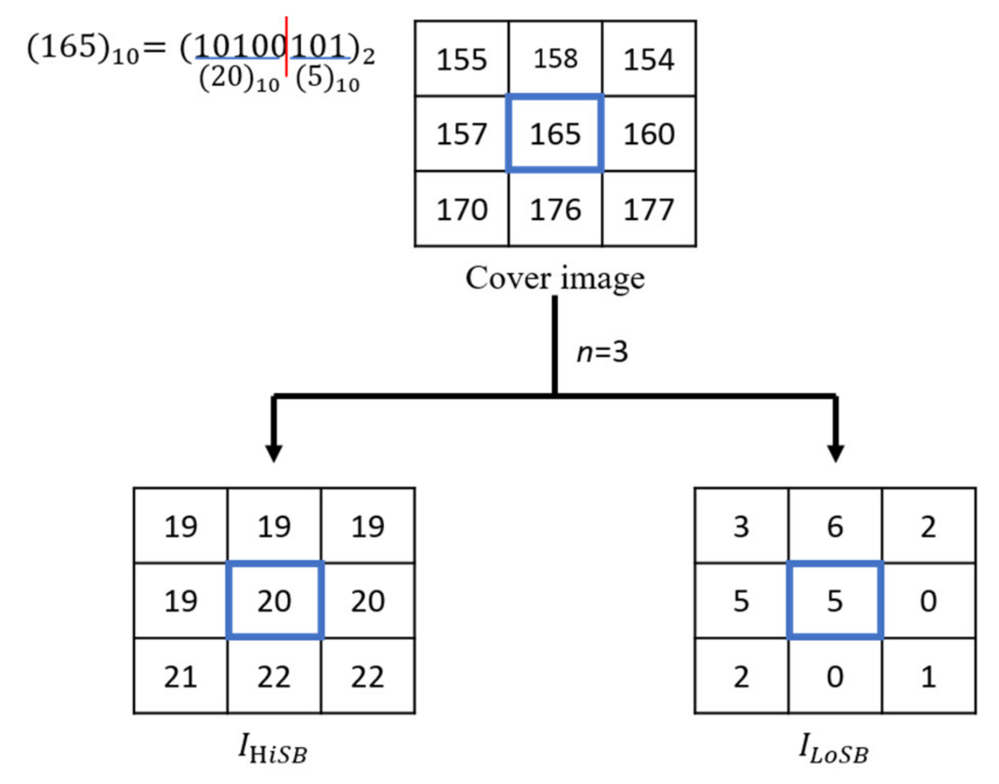
In the spatial domain, all pixels on the first layer correspond to their own corresponding values of the least significant bit (LSB); all pixels on the eighth layer correspond to their own corresponding values of the most significant bit (MSB). That is, the LoSBs contains the least significant n bits; the HiSBs contains the higher significant ($8-n$) bits. That is to say, in the eight-level bit plane, the original image pixel from the intensity value of level 1–127 is changed to 0, and the intensity value of the level 128–255 is changed to 1, and the resulting binary image is described below. The higher significant images of the higher layers are called higher significant bits and represented by $I_{HiSB}$ images, and the images of the lower significant of the lower layers are called lower significant bits (LoSBs). In this article, $I_{LoSB}$ images are represented. That is, the LoSBs contain the least significant n bits; the HiSBs contain the higher significant ($8-n$) bits. For example, a gray-scale pixel value is 155 = ${\left(10011011\right)}_2$. Assuming $n$ = 3, the pixel value of the original image pixel in this $I_{LoSB}$ image is ${\left(011\right)}_2$ = 3, and the pixel value in this $I_{HiSB}$ image is ${\left(10011\right)}_2$ = 19. Most of the information hiding techniques in spatial domain directly change the LSBs of the pixel value to achieve the embedding of secret data.

Both the significant-bit-difference expansion (SBDE) method proposed by Wang et al. [26] and the two-layer embedding (TLE) method proposed by Kumar and Jung at (2020) [27] utilize the HiSBs to achieve the information embedding and make the hiding methods more robust. Both the SBDE and TLE methods consider that the distortion of the $I_{HiSB}$ image should not be too large. It will only embed the secret message in the embedding area with low complexity. The measure of complexity complex is the variance of the pixel value on the $I_{HiSB}$ image. The smaller the variance, the higher the smoothness, which means that embedding secret information in this area will cause less distortion, therefore increasing the image visual quality. However, the SBDE method hides the data in the bit difference, resulting in severe image distortion. Therefore, the TLE method enhances the hiding performance both in image quality and embedding capacity.

2.1. Embedding Method of TLE

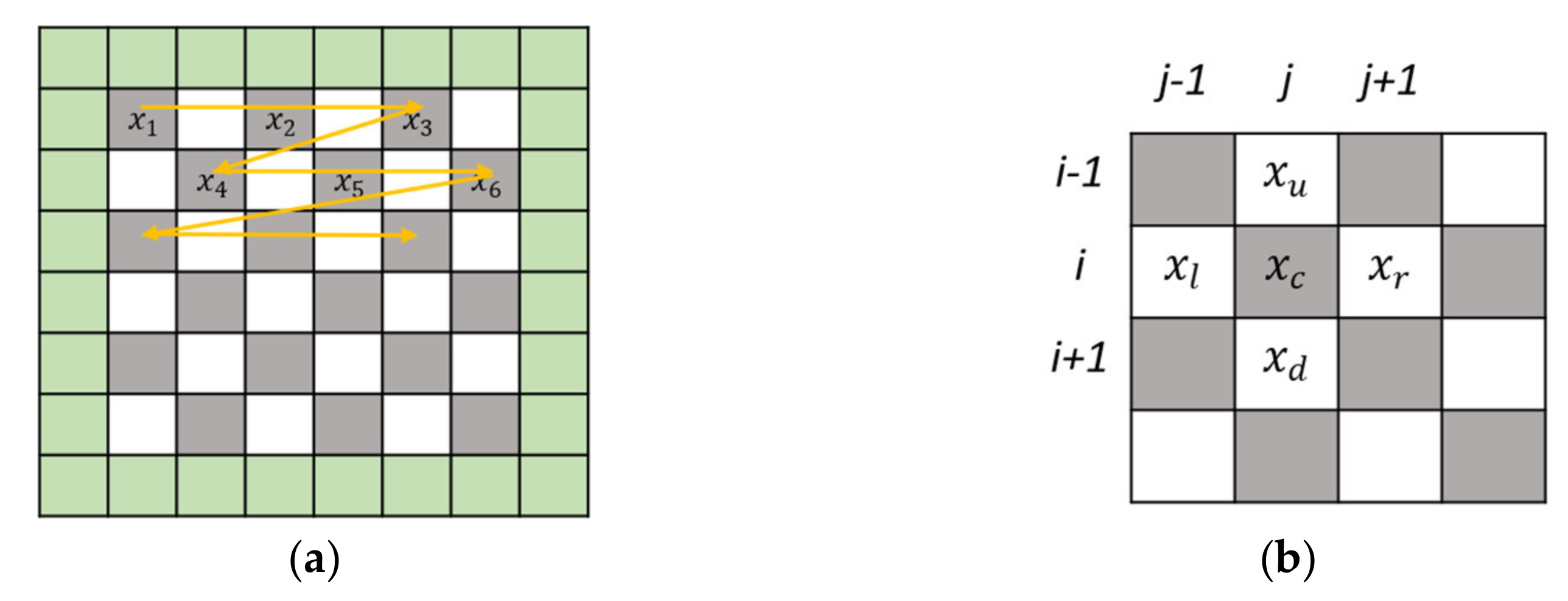
The TLE method first divides the pixel value of an $I_{HiSB}$ image into white and gray chessboards, as shown in Figure 1a. The secret information to be hidden is repeatedly embedded in the whole gray pixel values and then in the whole white pixel values. Figure 1a also shows that during the embedding process of the TLE method, the pixel values of the first column and the first row and the last column and last row of the $I_{HiSB}$ image will not be changed. The TLE embedding procedure is as follows.

Input: a gray-scale image $I$.

Output: a gray-scale stego image $I^{\prime }$.

Step 1. The binary representation of each pixel value in the gray-scale image $I$ is ($b_7,b_6,b_5,b_4,b_3,b_2,b_1,b_0)$,$b_i$ ∈{0, 1}. The cover image is decomposed into an image ($I_{HiSB}$) and an image ($I_{LoSB}$), where the pixel value of each pixel in the $I_{HiSB}$ image is $\{x$= ($b_7, \dots ,b_{n+2},b_{n+1},b_n)$ | $2^n\le x\le 2^8-1$}.

Step 2. For the convenience of description, let the $I_{HiSB}$ image be represented by the gray-scale pixel ($x_{i,j}$) in Figure 1b. In the $I_{HiSB}$ image, it is used as the carrier for embedding the secret message of the embedding binary. Let $x_c=x_{i,j}$; in Figure 1b, the white pixel values of the top, bottom, left and right of the pixel ($x_c$) are ($x_{i-1,j},x_{i+1,j},x_{i,j-1},x_{i,j+1}$). For the convenience of explanation, let $\left(x_u,x_d,x_l,x_r\right) = \left(x_{i-1,j},x_{i+1,j},x_{i,j-1},x_{i,j+1}\right)$. The vector $\left(x_u,x_d,x_l,x_r\right)$ is sorted according to the pixel value from small to large, and the result is $\left(x_{\pi \left(1\right)},x_{\pi \left(2\right)},x_{\pi \left(3\right)},x_{\pi \left(4\right)}\right)$.

Step 3. The local complexity of the pixel $x_c$ is defined as its surrounding four white pixel values $\left(x_{\pi \left(1\right)},x_{\pi \left(2\right)},x_{\pi \left(3\right)},x_{\pi \left(4\right)}\right)$, and the variance (${\sigma }_c^2$), as shown in Equation (1).

$${\sigma }_c^2=\frac{1}{4}{{\displaystyle \sum }}_{t=1}^4{\left({\mu }_c-x_{\pi \left(t\right)}\right)}^2,$$

(1)

where ${\mu }_c=\frac{1}{4} {{\displaystyle \sum }}_{t=1}^4{x}_{\pi \left(t\right)}$, is the average value of the white pixel values around the pixel $x_c$.

Step 4. The calculation of predictor:

Table 1. Three different predictor methods.

Predictors	Predictor Methods	1	2	3
$p_1$		$x_{\pi \left(1\right)}$	$\lfloor \frac{x_{\pi \left(1\right)}+x_{\pi \left(2\right)}+x_{\pi \left(3\right)}}{3}\rfloor$	$\lfloor \frac{x_{\pi \left(1\right)}+x_{\pi \left(2\right)}}{2}\rfloor$
$p_2$		$x_{\pi \left(4\right)}$	$\lfloor \frac{x_{\pi \left(2\right)}+x_{\pi \left(3\right)}+x_{\pi \left(4\right)}}{3}\rfloor$	$\lfloor \frac{x_{\pi \left(3\right)}+x_{\pi \left(4\right)}}{2}\rfloor$

lists three predictor methods suggested by Kumar and Jung. Each predictor will have a pair of predictors ($p_1, p_2$) used as a prediction error. Predictor method 1 will use the largest and smallest pixel values in the ordered vector ($x_{\pi \left(1\right)},x_{\pi \left(2\right)},x_{\pi \left(3\right)},x_{\pi \left(4\right)}$), which is a pair of extreme values neighbors of pixel $x_c$. The extreme value neighbors are $x_{\pi \left(4\right)}$ and $x_{\pi \left(1\right)}$ as predictors $p_1$ and $p_2$. The predictor method 2 is the most comprehensive predictor, which will use the four white neighbors of pixel $x_c$. Each predictor $p_1$ or $p_2$ will use the average of the three white neighbors to make predictions. The design of predictor method 3 puts the predictors between the extreme predictor method 1 and the comprehensive predictor method 2.

Step 5. Two-layer embedding (TLE) strategy: refers to the strategy that each pixel in the image ($I_{HiSB}$) can embed the secret data twice. In the first layer embedding program, the TLE strategy uses Equation (2) to embed the secret bit $s_1$ into the pixel $x_c$, and the method is: first calculate the first prediction error $e_1=x_c-p_1$, and then the to-be-embedded secret bit $s_1\in \left\{0,1\right\}$, as in Equation (2):

$$x_c^{\left(1\right)}=\left\{\begin{array}{c} x_c+s_1, if e_1=1\\ x_c+1, if e_1>1\\ x_c, if e_1<1\end{array}\right.$$

(2)

where $x_c^{\left(1\right)}$ is the intermediation value after embedding in the first layer.

Step 6. In the second embedding layer, the TLE method calculates the second prediction error $e_2=x_c^{\left(1\right)}-p_2$, and then uses Equation (3) to hide the secret bit $s_2\in \left\{0,1\right\}$ into $x_c^{\left(1\right)}$.

$$x_c^{\left(2\right)}=\left\{\begin{array}{c}{x}_c^{\left(1\right)}-s_2, if e_2=-1\\ x_c^{\left(1\right)}-1, if e_2<-1\\ x_c^{\left(1\right)}, if e_2>-1\end{array}\right.$$

(3)

where $x_c^{\left(2\right)}$ is the stego pixel value after embedding in the second layer.

The TLE method aims at the prediction error $e_1=1$, and then the pixel value $x_c$ on the original $I_{HiSB}$ image will add $s_1$. If the prediction error $e_2=-1$, then the pixel value on the $I_{HiSB}$ image will be the intermediation value $x_c^{\left(1\right)}$ subtracting $s_2$ after the first layer of the embedding procedure.

In the TLE strategy, the design predictor $p_2$ is always greater than the predictor $p_1$, so the predictor ($p_2$) embedded in the second layer can be modified to $p_2^{\prime }$ by Equation (4):

$$p_2^{\prime }=\left\{\begin{array}{c}{p}_2+1, if p_2=p_1\\ p_2, otherwise\end{array}\right.$$

(4)

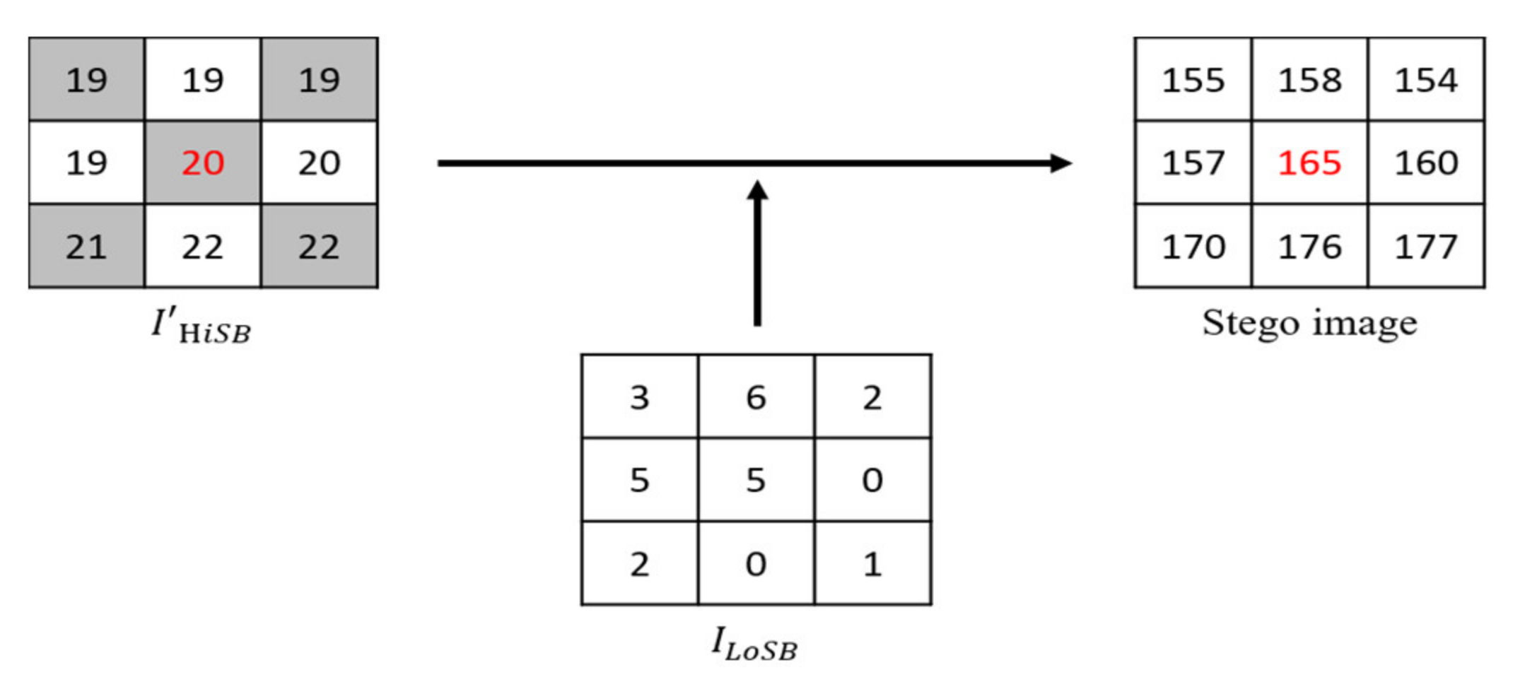
Step 7. The pixel of ${I^{\prime }}_{HiSB}$ is converted to binary, which is the original $\left(b_7, \dots ,b_{n+2},b_{n+1},b_n\right)$ and pixel of $I_{LoSB}$ converted to binary, which is the original ($b_n,b_{n-1},\dots ,b_0$) combined into a stego pixel, until all the pixels are combined into a gray-scale stego image $I^{\prime }$.

Step 8. Steps 2 to 7 are repeated to perform the TLE embedding method on the white pixel of $I_{HiSB}$.

Some auxiliary information is needed. The auxiliary information includes the following:

Location map (LM): To avoid the overflow/underflow problem and to lossless extract the secret message and restore the image recovery, the following Equation (5) is used to pre-process the image to generate a location map (LM). If $MIN\le x_c\le MAX \mathrm{where} MAX=2^{\left(8-n\right)}-1 \mathrm{and} MIN=0$, the location map $L{M}_{i,j}$ is represented by 0; if not MAX or MIN, $L{M}_{i,j}$ is represented by 1.

$$\begin{array}{c}{x}_{i,j}=\left\{\begin{array}{c}{x}_{i,j}-1, if x_{i,j}=MAX\\ x_{i,j}+1, if x_{i,j}=MIN\\ x_{i,j}, otherwise\end{array}\right. and \\ L{M}_{i,j}=\left\{\begin{array}{c}0,if x_{i,j}=MAX or MIN\\ 1,otherwise\end{array}\right.\end{array}$$

(5)

2.2. Embedding Example

The following example shows the method of TLE. Assuming that a gray-scale image $I$ has 3 × 3 pixels, its pixel value is shown in Figure 2. First, set $n=3$ is used to divide the cover image $I$ into 2 planes, namely $I_{HiSB}$ image and $I_{LoSB}$ image. Then, the $I_{HiSB}$ image is used as the secret carrier. Take the pixel value ($x_c$) of the $I_{HiSB}$ image as a carrier, which is 20. The following example illustrates the embedding process:

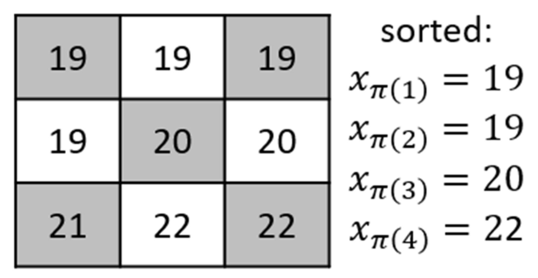
The TLE method sorts the up, down, left, and right pixel values of the pixel ($x_c$) to obtain the result: ($x_{\pi \left(1\right)},x_{\pi \left(2\right)},x_{\pi \left(3\right)},x_{\pi \left(4\right)}$) = (19, 19, 20, 22), as shown in Figure 3.

The TLE strategy first selects which predictor method to use and then judges whether embedding secret bit $s_1$ can be embedded in $x_c$ according to Equation (2). Then according to Equation (3) the TLE strategy judges whether or not the second layer of secret bit $s_2$ can be embedded.

Assume this example uses predictor method 1, that is, $(p_1,p_2)=(x_{\pi \left(1\right)}$,$x_{\pi \left(4\right)}$) = ($19, 22)$. Additionally, suppose $s_1=1$ and $s_2=1$, then the prediction error $e_1=x_c-p_1=20-19=1$ is calculated according to Equation (2); therefore, $x_c^{\left(1\right)}$ = $x_c+s_1$ $=20+1=21$, and this completes the secret data embedding of the first layer. Then, the prediction error $e_2=x_c^{\left(1\right)}-p_2=21-22=-1$ is calculated according to Equation (3) as well as $x_c^{\left(2\right)}=x_c^{\left(1\right)}-s_2=21-1=20$, and this completes the second layer embedding. The embedded $x_c^{\left(1\right)}$ is combined with the pixel value of $I_{LoSB}$ to complete the embedding process, as shown in Figure 4.

The TLE method has the possibility of keeping the pixel value unchanged after embedding. It not only reduces the distortion of the image but also increases the embedding capacity and then uses the secret data algorithm to extract the secret message to achieve the purpose of information hiding.

3. Proposed Method

The pixel value of the $I_{\mathit{HiSB}}$ image is prone to the strong correlation among pixels, that is, $x_c$ is very similar to $p_1$ and $p_2$. Once the condition that $p_1$ is always smaller than $p_2$ is established and the pixel $x_c$ is squeezed between the two predictors $(p_1,p_2)$, there is a high probability that $e_1=x_c-p_1$∈{0, 1} or $e_1=x_c-p_2$ ∈{−1, 0}. For $e_1=1$, the pixel $x_c$ can carry one secret bit $s_1$, and then if $e_2=x_c^{\left(1\right)}-p_2=-1$, then it again carries another secret bit $s_2.$ Even if two secret bits are carried, because $p_1$ ≤ $x_c^{\left(2\right)}$ ≤ $p_2$, the stego pixel value does not change much, and good image quality can be maintained. Accordingly, the embedding is somehow like a repeated oscillation effect. The effect comes from embedding 1 bit data to make the original $I_{HiSB}$ pixel $x_c$ approach the predictor $p_2$ and then embedding another 1 bit data to make the pixel $x_c$ approach the predictor $p_1$ in the reverse direction. The proposed method utilizes the repeated oscillation effect to increase the embedding capacity without affecting the distortion of the image. This research method proposed an embedding strategy, which is called the recurrent round-trip embedding strategy (referred to as double R-TES strategy), that the pixel $x_c$ after embedding secret data will move back and forth between the two predictors $(p_1,p_2)$. The R-TES strategy embeds performs $(t-1$) times of outbound/backbound embedding, so the pixel $x_c$ can carry 2$t$ bit data. At the same time, $t$ location map bits are also derived to record the embedding secret data such that the secret message can be completely extracted, and the pixel values of $I_{HiSB}$ image can be exactly recovered.

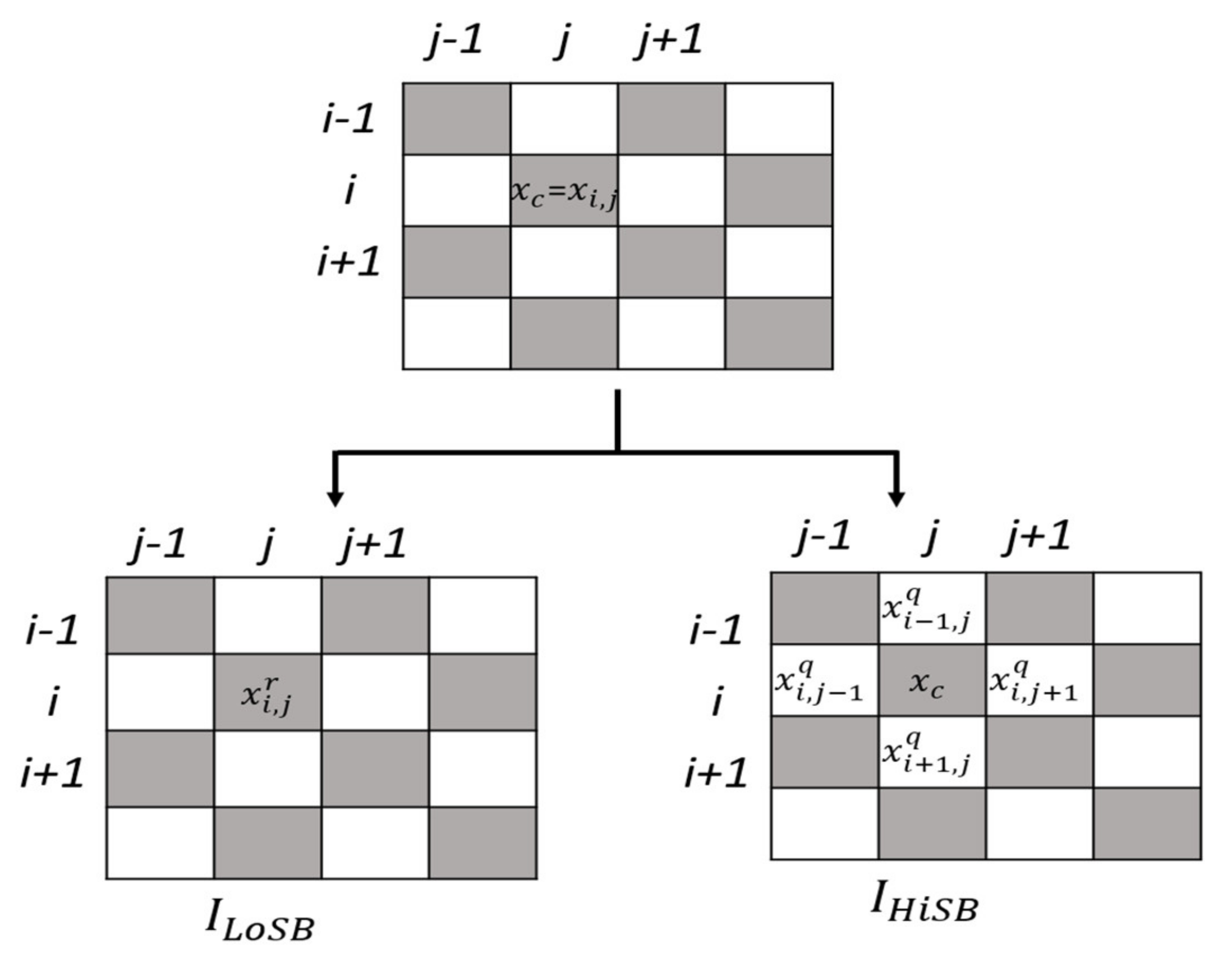
In the proposed information hiding scheme, the image $I$ is classified into two parts: un-embeddable and embeddable parts. The un-embeddable part is the pixel values of the first column and the first row and the last column and the last row. The remainder pixels of image $I$ can be used as cover image pixels to carry the secret data bits. Like the TLE method, we also first divide the pixel value of a quotient image into white and gray chessboards, as shown in Figure 5, and then the secret information to be hidden is repeatedly embedded in the pixel values of the gray grid first. According to the same embedding procedure, the hidden secret data are repeatedly embedded into the pixel values of the white grid.

3.1. Recurrent Robust Reversible Data Hiding (Triple-RDH) Embedding Method

Input: a gray-scale cover image $I$.

Output: a gray-scale stego image $I^{\prime }$.

Step 1. For the pixel in the embeddable area, the image $I$ is sheared into a quotient image (i.e., higher significant bit-plane image $I_{HiSB}$) and a remainder image (i.e., lower significant bit-plane image $I_{LoSB}$); that is, each embeddable pixel $x_i$ is divided into a quotient image pixel $x_i^q$ and a remainder image pixel $x_i^r,$ using the quotient and remainder operands, respectively, by Equation (6).

$$x_{i,j}^q=x_{i,j} \mathrm{div} 2^n; x_{i,j}^r=x_{i,j} \mathrm{mod} 2^n \mathrm{for} i=1, 2, \dots ,$$

(6)

for $=1, 2, \dots ,$ $H and j=1, 2, \dots ,W$, where $x_{i,j}\in I,$ $x_{i,j}^q \in I_{HiSB}$, and $x_{i,j}^r \in I_{LoSB}$; ‘div’ and ‘mod’ are the divide and modulo operations, respectively. Each quotient pixel $x_{i,j}^q$ of the image $I_{HiSB}$ is labeled into two image pixels of gray and white as in a chessboard-shaped chessboard.

Step 2. For each pixel $x_{i,j}^q\in I_{HiSB}$ on the chessboard image $I_{HiSB}$, let $x_c=x_{i,j}^q$. Then, the top, bottom, left, and right of the pixel $x_c$ are another-color pixel values that are different from the color of $x_{i,j}^q$. The pixel values are, respectively, $\left(x_{i-1,j}^q, x_{i+1,j}^q, x_{i,j-1}^q, x_{i,j+1}^q\right)\in I_{HiSB}.$ If $x_c=x_{i,j}^q$ is gray, then ($x_{i-1,j}^q, x_{i+1,j}^q, x_{i,j-1}^q, x_{i,j+1}^q$) is the four white neighboring pixels of $x_{i,j}^q$; if $x_c=x_{i,j}^q$ is white, then ($x_{i-1,j}^q, x_{i+1,j}^q, x_{i,j-1}^q, x_{i,j+1}^q$) is the four gray neighboring pixels of $x_{i,j}^q$.

Step 3. The sort() function is used to sort ($x_{i-1,j}^q, x_{i+1,j}^q, x_{i,j-1}^q, x_{i,j+1}^q$) in ascending order, and the result obtained is ($x_{\pi \left(1\right)},x_{\pi \left(2\right)},x_{\pi \left(3\right)},x_{\pi \left(4\right)}$).

$$\left(x_{\pi \left(1\right)},x_{\pi \left(2\right)},x_{\pi \left(3\right)},x_{\pi \left(4\right)}\right)=\mathrm{sort}\left(x_{i-1,j}^q, x_{i+1,j}^q, x_{i,j-1}^q, x_{i,j+1}^q\right)$$

(7)

The sort() function $\pi :\left\{1, 2, \dots , n\right\} \to \left\{1, 2, \dots , n\right\}$ is the unique one-to-one mapping. In the case of equal value, pixels are ordered by $\pi \left(k\right) <\pi \left(\mathcal{l}\right)$, if $x_{\pi \left(k\right)}$ = $x_{\pi \left(\mathcal{l}\right)}$ and k <$\mathcal{l}$.

Step 4. The local complexity of pixel $x_c$ is defined as the variance (${\sigma }_c^2$) of the surrounding four color pixel values ($x_{\pi \left(1\right)},x_{\pi \left(2\right)},x_{\pi \left(3\right)},x_{\pi \left(4\right)}$), as shown in Equation (8).

$${\sigma }_c^2=\frac{1}{4}{{\displaystyle \sum }}_{k=1}^4{\left({\mu }_c-x_{\pi \left(k\right)}\right)}^2,$$

(8)

where ${\mu }_c=\frac{1}{4} {{\displaystyle \sum }}_{k=1}^4{x}_{\pi \left(k\right)},$ which is the average value of the four color pixel values around pixel $x_c$.

Step 5. The recurrent round-trip embedding strategy (referred to as double R-TES strategy) is expressed. For the convenience of explanation, assume that $x_c$ is a gray pixel at this time:

$$x_c^{\left(out\right)}=\left\{\begin{array}{c} x_c+s^{out}, if e^{out}=p{p}_1\\ x_c+1, if e^{out}>p{p}_1\\ x_c, if e^{out}<p{p}_1\end{array}\right.$$

(9)

$$x_c^{\left(back\right)}=\left\{\begin{array}{c}{x}_c^{\left(out\right)}-s^{in}, if e^{back}=p{p}_2\\ x_c^{\left(out\right)}-1, if e^{back}<p{p}_2\\ x_c^{\left(out\right)}, if e^{back}>p{p}_2\end{array}\right.$$

(10)

Step 6. $p{p}_1$ and $p{p}_2$ are two predetermined peak points. According to the experimental statistics of this research, setting $p{p}_{1 }$= 1 and $p{p}_2$= −1 will make the embedding capacity more effective.

Step 7. Then, determine whether $x_c^{\left(back\right)}$ can be used a carrier to embed information: compare the gray pixel $x_c$ of the original cover image with the gray pixel $x_c^{\left(back\right)}$ that has been embedded back and forth $t_w$. times (that is, at most $2t_w$ bits of information have been hidden). If $x_c^{\left(back\right)}=x_c$, this means that the process goes back to Step 6, and the recurrent round-trip embedding strategy can be used again and again to let $x_c^{\left(back\right)}$ be the carrier and have the opportunity to embed more than two secret data bits. If ${x^{\prime }}_c^{\left(q\right)}=x_c^{\left(back\right)}$, then go to Step 8.

Step 8. When the last embeddable gray pixel $x_c=x_{i,j}^q$ of $I_{HiSB}$, i.e., $i=H-1$ and $j=W-1$, has been processed, the procedure in a zig-zag canning manner starts to proceed to the first embeddable white pixel $x_{i,j}^q$, i.e., $i=$2 and $j=$3 of $I_{HiSB}$, until all white pixels are processed to embed secret data.

Step 9. The final process is to merge the quotient image pixels ($8-n$ HiSBs) and the remainder image pixels $(n$ LoSBs) back to the gray-scale stego image pixels by Equation (11) and return the stego image $I^{\prime }.$

$$x_c^{\prime }={x^{\prime }}_c^{\left(q\right)} \mathrm{mul} 2^n+x_i^r,$$

(11)

where ‘mul’ stands for the multiplier operator.

This research will generate some extra information: the location map $L{M}_{i,j}^{\left(t\right)}$ and the parameters for hiding data bits. The lossless compression technology “Arithmetic Coding” is used to compress the location map to a length of (${\mathcal{l}}_{CLM}$) << $t\times H\times W$, and the least significant bit (LSB) substitution method is used with other additional information to hide the end of the image. The function of location map $L{M}_{i,j}^{\left(t\right)}$ has the following two situations:

CASE 1: When the recursive parameter $t$= 1, the location map $L{M}_{i,j}^{\left(1\right)}$ is used to avoid overflow/underflow problems and lossless extraction of secret message to restore the image.

$$\begin{array}{c}{x}_{i,j}=\left\{\begin{array}{c}{x}_{i,j}-1, if x_{i,j}=MAX\\ x_{i,j}+1, if x_{i,j}=MIN\\ x_{i,j}, otherwise\end{array}\right. and \\ L{M}_{i,j}^{\left(1\right)}=\left\{\begin{array}{c}0,if x_{i,j}=MAX or MIN\\ 1,otherwise\end{array}\right.\end{array}$$

(12)

CASE 2: When the recursive parameter $t$> 1, the location map $L{M}_{i,j}^{\left(t\right)}$ is used to allow the receiving end to recover smoothly in the process of extracting the information, and every pixel must be recorded how many times the triple-RDH embedding method have been carried out on the pixel; every time it is carried out, it hides a 2-bit data with $L{M}_{i,j}^{\left(t\right)}$= 1, otherwise $L{M}_{i,j}^{\left(t\right)}$= 0.

In addition to the location map, the parameters $n,t_g, t_w, S_{end}$ are required as additional information, where $n\left\{1,2, 3, 4\right\} ,$ using two bits to encode the $n$ value and $t_g, t_w\left\{1,2, 3, 4\right\}$ using four bits to encode the ($t_g, t_w$) values. The index value $S_{end}$ is recorded to distinguish the boundary of extra information and the secret message $S$. The position of the last embedded pixel value is found out when extracting the extra information.

The extra information items and the required bit sizes are shown in

Table 2. The extra information items and required bit sizes.

Extra Information Items	Required Bit Sizes (Bits)
$n$	2
$t_g$	2
$t_w$	2
The length of the $L{M}_{i,j}^{\left(t\right)}$ where t∈{$t_g, t_w\}$	$\lceil lo{g}_2\left(H\times W\right)\rceil \times (t_g+t_w$)
Compressed location maps	$l_{clm}{}^k$ where k = 1, 2, …, $(t_g+t_w$)
Index value $S_{end}$	$\lceil lo{g}_2\left(H\times W\right)\rceil$

. It is required to embed the overhead information at the end of the cover image by exploiting the LSB method. The size of extra information is $\left(6+\lceil lo{g}_2\left(H\times W\right)\rceil +{{\displaystyle \sum }}_k^{ (t_g+t_w)}{l}_{clm}{{}^k}_{}\right)$ bits, and the LSB, which has been replaced by the extra information, is represented as $H_{LSB}$.

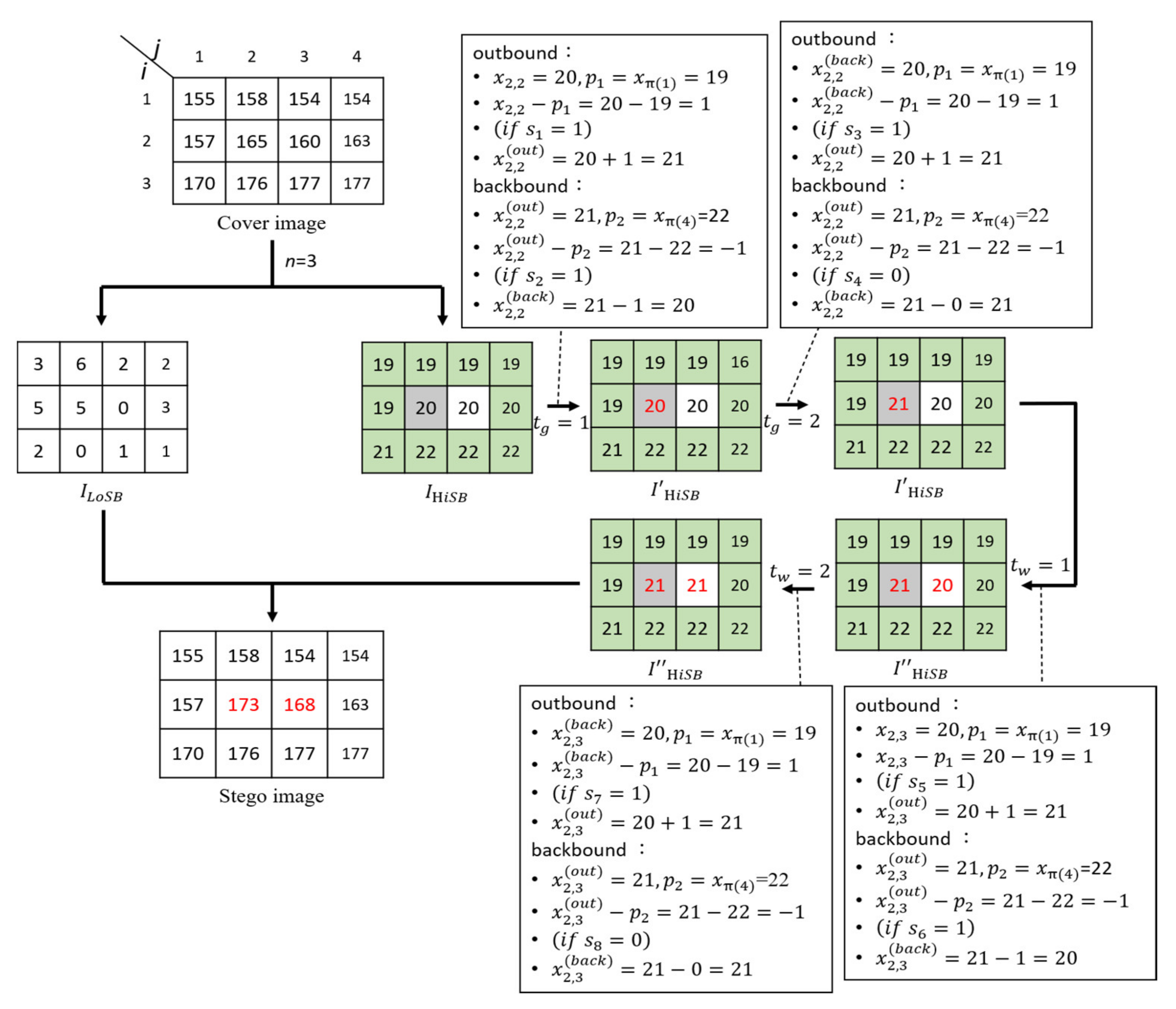
3.2. Embedding Example

We take a cover image with 12 pixels as shown in Figure 6 to illustrate the data embedding procedure. The cover image is split into two images, $I_{HiSB}$ and $I_{LoSB},$ through Equation (6). The quotient pixels in the $I_{HiSB}$ image are divided into gray pixels and white pixels in a chessboard manner. Let us suppose there is a secret bitstream $S=$ $s_1{s}_2{s}_3{s}_4{s}_5{s}_6{s}_7{s}_8$ = “1110 1110” and the predictor method 1 is used in this example.

First, the recurrent round-trip embedding strategy (double R-TES) for the gray pixel is used to calculate the prediction error $e^{out}=x_{2,2}-p_1=20-19=1$. According to Equation (9), the first secret bit $s_1=1$ is taken out from the secret message 𝑆, and then $x_{2,2}^{\left(out\right)}=20+1=21$ is calculated. This completes the embedding of the outbound value $x_1^{\left(out\right)}=21$ and then calculates the backbound value $e^{back}=x_{2,2}^{\left(out\right)}-p_2=21-22=-1$. According to Equation (10), the secret bit $s_2=1$ is embedded to obtain the backbound value $x_{2,2}^{\left(back\right)}=21-1=20$. It is observed that $x_{2,2}^{\left(back\right)}=x_{2,2}$. According to the double R-TES embedding strategy, the gray pixel $x_{2,2}$ can continue embedding more secret data bits. At this time, the recursive parameter $t_g=2$. According to Equation (6), the prediction error $e^{out}=x_{2,2}^{\left(back\right)}-p_1=20-19=1$, and $s_3=1$ is taken from the message S again to make $x_{2,2}^{\left(out\right)}=20+1=21$. According to Equation (7) again, $e^{back}=x_{2,2}^{\left(out\right)}-p_2=21-22=-1$. After $s_4=0$ is embedded into $x_{2,2}^{\left(out\right)}$, the result $x_{2,2}^{\left(back\right)}=21-0=21$ is obtained, and the embedding of the backbound is completed.

Since $x_{2,2}^{\left(back\right)}\ne x_{2,2}$, in this example, only two pixels $x_{2,2} \mathrm{and} x_{2,3}$ are embeddable, so Step 8 is executed to start embedding the message in another embeddable white pixel $x_{2,3}$.

Table 3. White pixel value and the changes of various values in the embedding procedure.

$\mathbf{Recursive} \mathbf{Parameter} {\mathit{t}}_{\mathit{w}}$	Original Pixel	Predictor	e	S	Stego Pixel
$t_w=1$	$x_{2,3}=20$	$p_1=19$	$e^{out}=1$	$s_5=1$	$x_{2,3}^{\left(out\right)}=21$
	$x_{2,3}^{\left(out\right)}=21$	$p_2=22$	$e^{back}=-1$	$s_6=1$	$x_{2,3}^{\left(back\right)}=20$
$t_w=2$	$x_{2,3}^{\left(back\right)}=20$	$p_1=19$	$e^{out}=1$	$s_7=1$	$x_{2,3}^{\left(out\right)}=21$
	$x_{2,3}^{\left(out\right)}=21$	$p_2=22$	$e^{back}=-1$	$s_8=0$	$x_{2,3}^{\left(back\right)}=21$

shows the embedding process in which the proposed triple-RDH is applied to embed the remainder data $“s_5{s}_6{s}_7{s}_8”$ into the white pixels.

3.3. Extracting the Message and Restoring the Original Image

At this stage, the receiver uses the instructions of the additional information to extract the secret message embedded in the stego image $I^{\prime }$ according to the reverse operation method of the embedding procedure to recover the original image $I$.

Like the recurrent robust reversible data hiding (triple-RDH) method in this study, we distinguish the stego image ($I^{\prime }$) into embeddable and un-embeddable areas: the pixel values of the first column, first row, last column, and last row of the stego image are the un-embeddable part. For each embeddable stego pixel $y_i$, the quotient operation is $y_i^q$ = $y_i$div $2^n$.

As mentioned above, since we need to reverse the hidden method to extract the secret message and recover the original pixel value, we need to extract the message bits from the white pixels with the recursive parameter $t_w$ first until all the secret messages hidden in the white pixels are retrieved and the white pixel value is recovered, then the recursive parameter $t_g$ is used to start message extraction and recovery of gray pixel value. In the following extraction equation, we take the recursive parameters $t_w=2$ and $t_g=2$ as an illustration.

The receiver will use the following Equations (13) and (14) in the information extraction and recovery procedure of the pixel value. When $t_w=2$, the white pixel value will be processed first.

$$x_c^{\left(back\right)}=\left\{\begin{array}{c}{y}_i^q+1,if e^{back}<-2\\ y_i^q+1,if e^{back}=-2\\ y_i^q ,if e^{back}=-1\\ y_i^q ,if e^{back}>-1\end{array}\right. and s_4=\left\{\begin{array}{c}none,if e^{back}<-2\\ 1,if e^{back}=-2\\ 0,if e^{back}=-1\\ none,if e^{back}>-1\end{array}\right.$$

(13)

$$x_c^{\left(out\right)}=\left\{\begin{array}{c}{x}_c^{\left(back\right)} ,if e^{out}<1\\ x_c^{\left(back\right)} ,if e^{out}=1\\ x_c^{\left(back\right)}-1,if e^{out}=2\\ x_c^{\left(back\right)}-1,if e^{out}>2\end{array}\right. and s_3=\left\{\begin{array}{c}none,if e^{out}<1\\ 0,if e^{out}=1\\ 1,if e^{out}=2\\ none,if e^{out}>2\end{array}\right.$$

(14)

Then, when $t_w=1$, the message extraction and recovery procedure of pixel value use the following Equations (15) and (16) to recovery white pixel value and extract the secret message until all the white pixel values are restored and the secret message is extracted.

$$x_c^{\left(back\right)}=\left\{\begin{array}{c}{x}_c^{\left(out\right)}+1,if e^{back}<-2\\ x_c^{\left(out\right)}+1,if e^{back}=-2\\ x_c^{\left(out\right)} ,if e^{back}=-1\\ x_c^{\left(out\right)} ,if e^{back}>-1\end{array}\right. and s_2=\left\{\begin{array}{c}none,if e^{back}<-2\\ 1,if e^{back}=-2\\ 0,if e^{back}=-1\\ none,if e^{back}>-1\end{array}\right.$$

(15)

$$x_c=\left\{\begin{array}{c}{x}_c^{\left(back\right)} ,if e^{out}<1\\ x_c^{\left(back\right)} ,if e^{out}=1\\ x_c^{\left(back\right)}-1,if e^{out}=2\\ x_c^{\left(back\right)}-1,if e^{out}>2\end{array}\right. and s_1=\left\{\begin{array}{c}none,if e^{out}<0\\ 0,if e^{out}=0\\ 1,if e^{out}=1\\ none,if e^{out}>1\end{array}\right.$$

(16)

After completing the extraction of the white pixel value and the recovery of white pixel value, the information extraction and the recovery program procedure of the pixel value again use Equations (13) and (14) (at this time $t_g=2$), and Equations (15) and (16) (at this time $t_g=1$) are used to restore the gray pixel value and take out the secret message in sequence.

After extracting the hidden information, the location map (LM) is separated and decompressed into the original form, and the obtained image is reprocessed using Equation (17) to obtain the cover image.

$$x_c=\left\{\begin{array}{c}{x}_c+1, if x_c=MAX-1 and L{M}_{i,j}=0\\ x_c-1, if x_c=MIN+1 and L{M}_{i,j}=0\\ x_c, otherwise\end{array}\right.$$

(17)

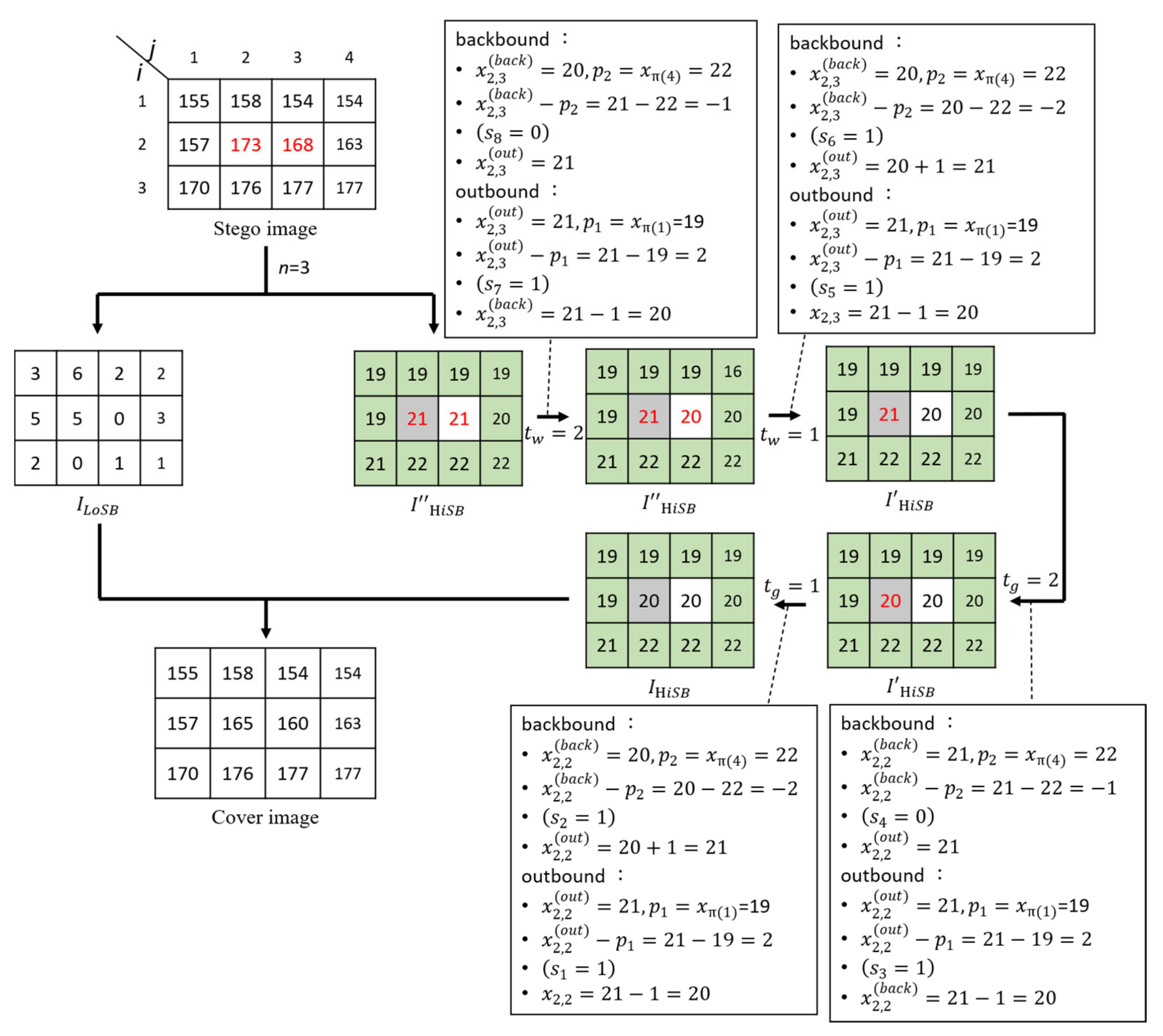
3.4. Extraction Example

The extraction process is exactly the reserve of the embedding process, so the message extraction and recovery procedures of the pixel value only need to be reversed. The following is an example of the extraction process:

First, take a stego image in Figure 7 and use Equation (6) to split it into two images ${I^{″}}_{HiSB}$ and $I_{LoSB}$. The embeddable pixel in the image ${I^{″}}_{HiSB}$ is divided into a gray pixel and a white pixel in a chessboard manner. First, the extract extraction for the white pixel and calculate the backbound prediction error $e^{back}=x_{2,3}^{\left(back\right)}-p_2=21-22=-1$, and according Equation (13), $s_8=0$, and $x_{2,3}^{\left(back\right)}$ is unchanged; therefore, $x_{2,3}^{\left(out\right)}=20+1=21$. Next, calculate the outbound prediction error so that $e^{out}=x_{2,3}^{\left(out\right)}-p_1=21-19=2$. According to Equation (14), $s_7=1$, and $x_{2,3}^{\left(out\right)}$ subtract 1 to restore the pixel value, so $x_{2,3}^{\left(back\right)}=21-1=20$. This completes the extraction of the outbound journey. Then, when the recursive parameter $t_w=1$, the backbound prediction error is also calculated, so that $e^{back}=x_{2,3}^{\left(back\right)}-p_2=20-22=-2$, which is expressed according to Equation (15); $s_6=1$, and add 1 to $x_{2,3}^{\left(back\right)}$ to restore the pixel value, so $x_{2,3}^{\left(out\right)}=20+1=21$. Finally, calculate the outbound prediction error so that $e^{out}=x_{2,3}^{\left(out\right)}-p_1=21-19=2$. According to Equation (16), $s_5=1$, and $x_{2,3}^{\left(out\right)}$ subtract 1 to restore the pixel value, so $x_{2,3}=21-1=20$. Finally, the secret bitstream extracted from the white pixels is as $s_5{s}_6{s}_7{s}_8=$ “1110”, and the pixel values are also restored.

In this example, there are only two pixels $x_{2,2} \mathrm{and} x_{2,3},$ so the next step is to extract the information from the gray pixel $x_{2,2}$ when the recursive parameter $t_g=2$. In order to simply express the extraction process,

Table 4. Gray pixel value and changes in various values in the extraction process.

$\mathbf{Parameter} {\mathit{t}}_{\mathit{g}}$	Stego Pixel	Predictor	Prediction Error e	Secret Bit	Restored Pixel
$t_g=2$	$x_{2,2}^{\left(back\right)}=21$	$p_2=22$	$e^{back}=-1$	$s_4=0$	$x_{2,2}^{\left(out\right)}=21$
	$x_{2,2}^{\left(out\right)}=21$	$p_1=19$	$e^{out}=2$	$s_3=1$	$x_{2,2}^{\left(back\right)}=20$
$t_g=1$	$x_{2,2}^{\left(back\right)}=20$	$p_2=22$	$e^{back}=-2$	$s_2=1$	$x_{2,2}^{\left(out\right)}=21$
	$x_{2,2}^{\left(out\right)}=21$	$p_1=19$	$e^{out}=2$	$s_1=1$	$x_{2,2}^{\left(back\right)}=20$

is used to show the changes in the values of the gray pixel during the extraction process to extract the secret bitstream $s_1{s}_2{s}_3{s}_4=$ “1110”. Figure 7 illustrates the whole extraction and recovery processes.

4. Experimental Results

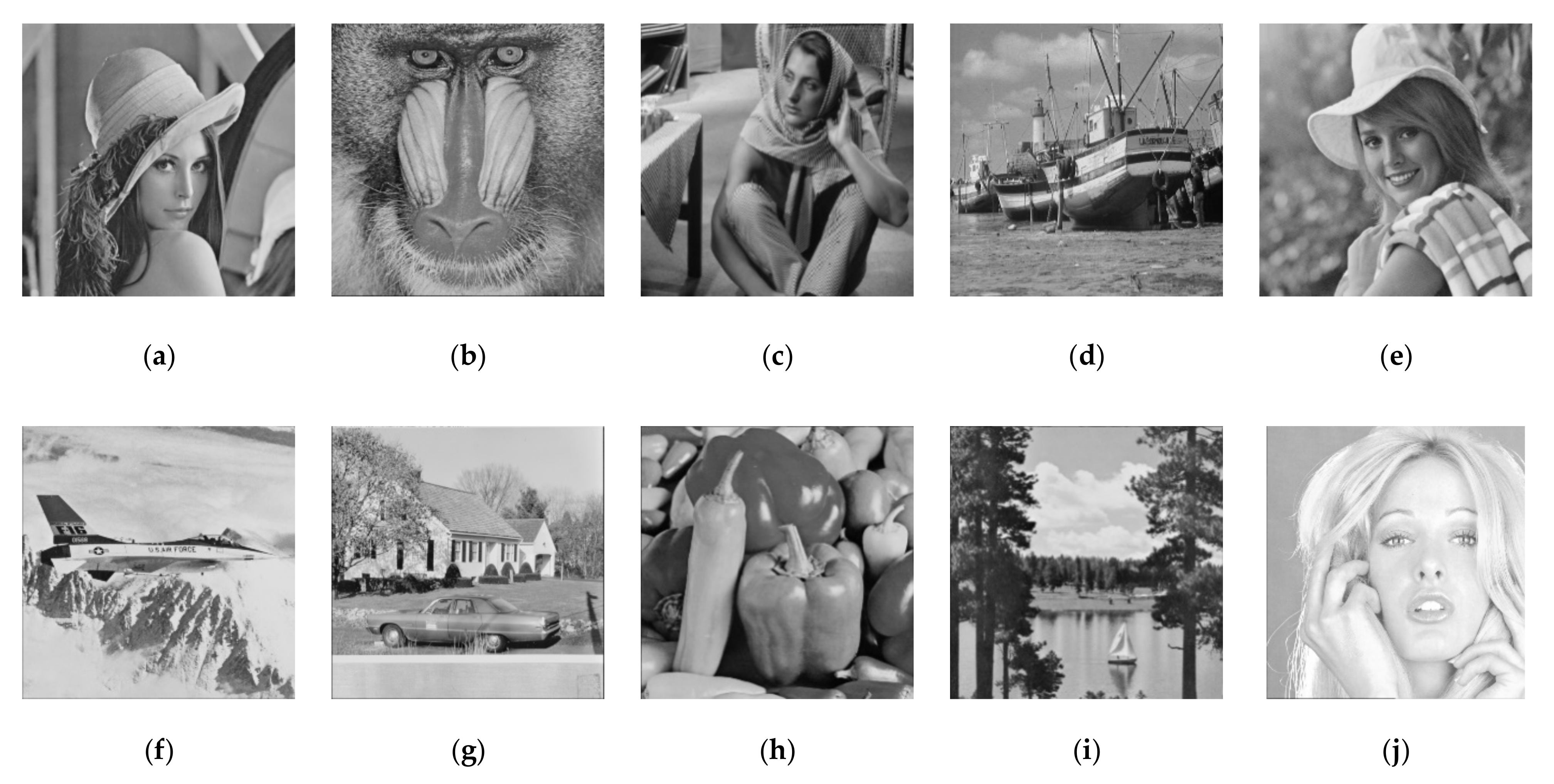
The hardware device used by our proposed recurrent robust reversible data hiding (triple-RDH) method is i7 with a solid-state disk with 16GB of memory. The operating system is Win10, and the tool developed is MATLAB. Ten 512 × 512 gray-scale images (“Lena”, “Baboon”, “Barbara”, “Boat”, “Elaine”, “F16”, “House”, “Pepper”, “Sailboat”, and “Tiffany”) are used as the test images, as shown in Figure 8. The secret data are binary string generated by a random function.

The following two evaluation metrics are used in our experiment: embedding capacity (EC) and peak signal-to-noise ratio (PSNR). EC represents the amount of secret data that can be embedded in the image, usually calculated in bits. The maximum embedding capacity refers to the maximum amount of data that can be embedded in an image. The PSNR computes the peak signal-to-noise ratio, in decibels, between two images. The higher the PSNR, the better, indicating that the stego image is highly undetectable. The calculation method of PSNR is $PSNR=10\times {\log }_{10}\left(\frac{MA{X}^2}{MSE}\right)$, where MAX is the maximum possible pixel value of the image. The method in this article is mainly based on the gray-scale image, so MAX is 255, and MSE is the mean square error, calculated by $MSE=\frac{1}{H\times W}{\displaystyle \sum }_{i=0}^{H-1}{\displaystyle \sum }_{j=0}^{W-1}{\left[I\left(i,j\right)-I^{\prime }\left(i,j\right)\right]}^2$, where H is the length of the picture, W is the width of the picture, $i, j$ are the pixel value positions, $I$ is the cover image, and $I^{\prime }$ is the stego image.

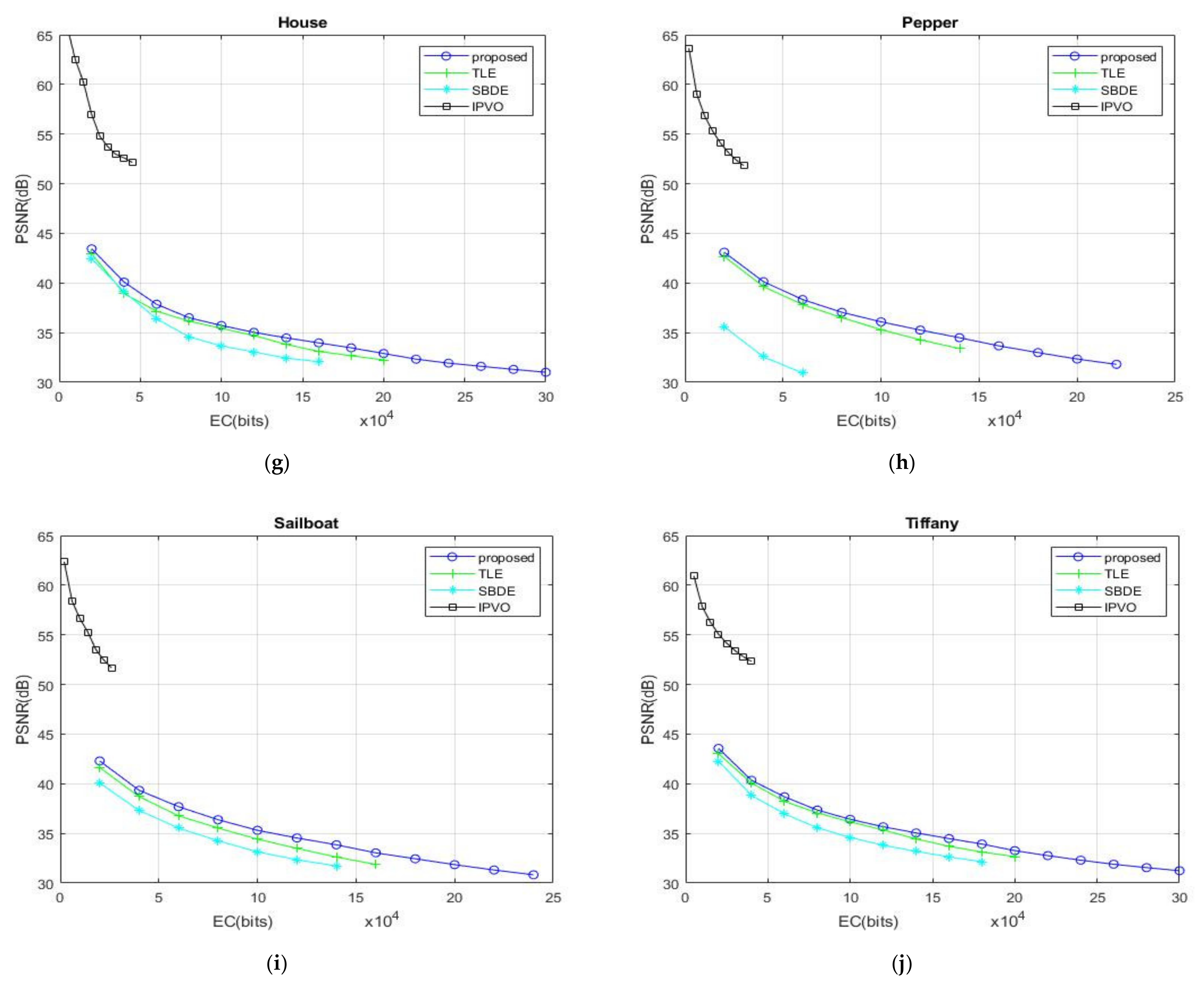
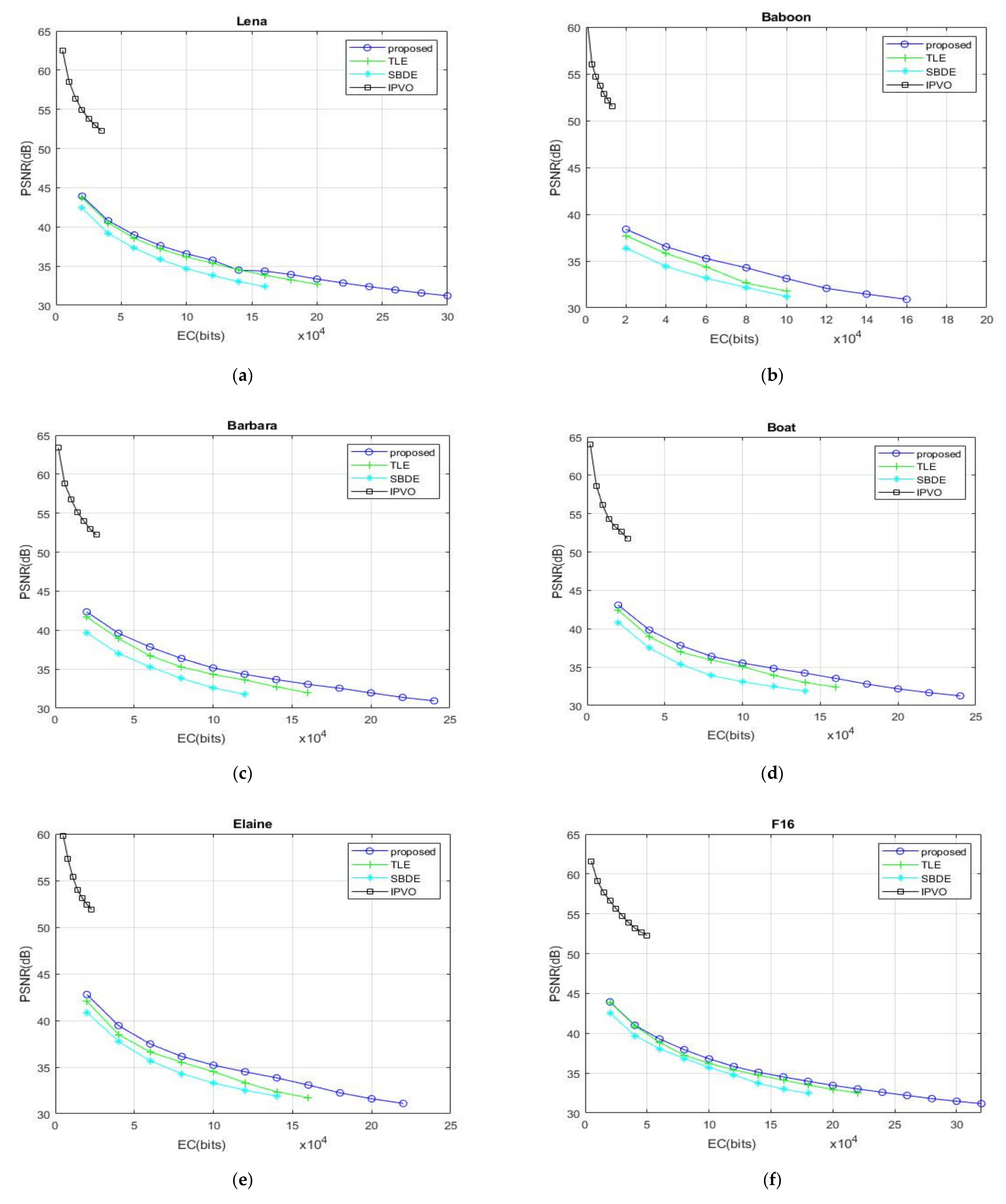
Figure 9 presents the experimental results of our proposed recurrent robust reversible data hiding (triple-RDH) method. Among the predictor methods used, predictor method 2 shows better experimental results than other predictor methods, so the proposed triple-RDH method chooses the predictor method 2 in all experiments. Additionally, we choose to compare with SBDE (significant-bit-difference expansion) [26], TLE (two-layer embedding) [27], and IPVO (improved pixel-value ordering) [22], because the TLE method, SBDE method, IPVO method, and proposed triple-RDH method are all based on prediction error expansion (PEE) technique.

In Figure 9, compared with the other three methods, it can be clearly seen that the EC of our proposed method is significantly larger than the other methods. In terms of PSNR, in addition to the IPVO method, the triple-RDH method we proposed is also slightly higher than that of TLE method and SBDE method.

Take the “Lena” image in Figure 9a and

Table 5. The comparison of embedding EC and PSNR values by the proposed triple-RDH method and TLE method with 10 standard images on the three predictor methods.

Prediction Method		1		2		3
Metrics		EC	PSNR	EC	PSNR	EC	PSNR
Lena	proposed	305,801	31.28	310,732	31.04	303,018	31.15
	TLE	203,243	32.38	214,166	32.35	207,599	32.27
Baboon	proposed	159,911	31.92	171,742	30.61	164,421	31.1
	TLE	105,668	32.53	117,025	31.16	111,388	31.65
Barbara	proposed	234,763	31.78	241,413	30.91	232,491	31.3
	TLE	155,623	32.71	165,488	31.82	158,707	32.21
Boat	proposed	244,807	31.34	258,190	30.92	246,237	31.02
	TLE	161,138	32.16	178,000	31.93	169,069	31.91
Elaine	proposed	229,595	30.94	234,097	30.79	221,368	30.76
	TLE	151,255	31.63	161,605	31.67	151,892	31.5
F16	proposed	317,728	31.43	324,187	31.12	316,406	31.23
	TLE	211,024	32.67	221,563	32.48	215,128	32.51
House	proposed	277,561	31.6	300,106	31.01	289,155	31.18
	TLE	184,380	32.68	203,994	32.17	195,964	32.29
Pepper	proposed	226,675	31.78	227,657	31.64	220,866	31.65
	TLE	149,081	32.66	157,962	32.72	151,723	32.6
Sailboat	proposed	228,441	31.4	240,060	30.82	228,850	31
	TLE	149,924	32.2	165,010	31.71	156,430	31.81
Tiffany	proposed	310,258	31.23	306,476	31.13	301,025	31.12
	TLE	205,499	32.33	211,059	32.42	206,334	32.29

as an example; you can see that the maximum EC of the TLE method has 214,116 bits, the maximum EC of the SBDE method has 179,793 bits, the maximum EC of IPVO method is 38,755 bits, and the maximum EC of our proposed triple-RDH method can be as high as 310,732 bits, which is 1.45 times and 1.73 times more than that of the TLE method and the SBDE method, respectively; the maximum EC of our proposed method is eight times that of the IPVO method.

When the “Lena” image in Figure 9a has the EC = 20,000 bits, the PSNR values of the TLE method, the SBDE method, the IPVO method, and the proposed triple-RDH methods are 43.72, 42.41, 54.91, and 43.94 dB, respectively. When the embedded information is added up to 40,000 bits, the PSNR values of the TLE method, the SBDE method, and our proposed triple-RDH method are 40.52, 39.19, and 40.81 dB, respectively. At this time, the IPVO method is not capable of hiding 40,000 bits into the “Lena” image. Let us observe again if the EC is increased to 60,000 bits in the “Lena” image, the PSNR values of the TLE method, the SBDE method, and our proposed triple-RDH method are 38.55, 37.28, and 38.98 dB, respectively. It can be seen that our triple-RDH method is higher than the TLE method and the SBDE method in terms of PSNR value. The EC of the IPVO method cannot reach 40,000 bits, but we can easily embed more than 60,000 bits, and our advantage in the embedding capacity is great.

Let us observe more complicated images, such as the “Baboon” image in Figure 9b and Table 5 as an example. It can be seen that the maximum EC of the TLE method is 117,025 bits, the maximum EC of the SBDE method is 105,149 bits, the maximum EC of the IPVO method is 13,736 bits, and the maximum EC of our proposed triple-RDH method is 171,742 bits, which is much higher than the other three methods, which are 1.46 times and 1.63 times the TLE method and the SBDE method, respectively. The maximum EC of the proposed method is 12 times that of the IPVO method.

When the “Baboon” image in Figure 9b is embedded in 20,000 bits, the PSNR value of the TLE method is 39.1 dB, the PSNR value of the SBDE method is 36.39 dB, and the PSNR value of the triple-RDH method we proposed has 39.8 dB, but the IPVO method is incapable of carrying 20,000 bits. When the EC is increased to 40,000 bits, the PSNR values of the TLE method, the SBDE method, and the proposed triple-RDH method are 36.73, 34.42, and 37.6 dB, respectively. When the EC is increased up to 60,000 bits, the PSNR values of the TLE method, the SBDE method, and the proposed triple-RDH method are 35.01, 33.16, and 36.08 dB, respectively. It can also be seen that the PSNR value of our proposed method is higher than those of the TLE and SBDE methods. In the image of the “Baboon”, the EC of the IPVO method is less than 20,000, so the PSNR cannot be compared.

Let us observe the average maximum EC and image quality PSNR of the ten test images in Figure 9a–j and Table 5. It can be seen that the average maximum EC of the TLE method is 179,587 bits, the average maximum EC of the SBDE is 149,298 bits, and the average maximum EC of IPVO is 33,465 bits. The average maximum EC of the triple-RDH method we proposed is 261,466 bits. Even in any image in Figure 9, there is an obvious difference in the embedding capacity. We have a great advantage in the embedding capacity, and the PSNR value tends to be flat when the embedding capacity is higher. Compared with other methods, especially the PSNR of IPVO presents a steeper downward trend.

In Figure 9a–j, when the EC is 20,000 bits, the PSNR values of TLE, SBDE, IPVO, and the proposed triple-RDH method are 42.39, 40.31, 54.34 B, and 42.89 dB on average, respectively. When the EC is 40,000 bits, the average PSNR values of TLE, SBDE, IPVO, and the proposed triple-RDH method are 39.24, 37.34, 52.71, and 39.89 dB, respectively. When the EC is 60,000 bits, the average PSNR values of TLE, SBDE, IPVO, and the proposed triple-RDH method are 37.35, 35.47, and 38.04 dB, respectively; However, the IPVO method is incapable of hiding anything at this time. The PSNR value of the proposed triple RDH method is slightly higher than those of the average PSNR values of the TLE and SBDE methods.

From Table 5, our proposed triple-RDH method using predictor method 2 has a higher EC than Predictor methods 1 and 3. In the “Lena” image, the EC of our triple-RDH method is 4931 bits higher than that of the method using Predictor method 1, and also 7714 bits higher than that of the method using predictor method 3. Table 5 is also a comparison table of our proposed triple-RDH method and TLE on the different predictor methods in terms of EC and PSNR metrics. It can be found that the maximum EC of all predictor methods of our proposed method is higher than that of the TLE method. At the maximum EC, the PSNR value of our proposed triple RDH method with predictor Method 2 is only slightly lower than that of the TLE method by 1.31 dB; the PSNR value of our proposed triple RDH method using predictor Method 3 is slightly lower by 1.12 dB; the PSNR value of our proposed triple RDH method using predictor method 1 is slightly lower by 1.1 dB.

Table 6. Comparison of the performance of our triple-RDH method on images “Baboon” and “F16” with different n and different peak points.

Image		Baboon						F16
Prediction Method		1		2		3		1		2		3
Metrics		EC	PSNR	EC	PSNR	EC	PSNR	EC	PSNR	EC	PSNR	EC	PSNR
$n=1$	(0, −1)	38,239	46.34	53,738	42.94	49,517	44.49	151,726	44.29	171,459	42.84	158,831	43.49
	(1, −1)	43,496	45.93	56,084	42.78	52,291	44.17	182,186	44.2	204,695	42.99	190,126	43.51
	(1, 0)	39,552	46.51	55,228	42.95	50,813	44.58	162,201	44.85	179,161	42.88	175,669	43.76
$n=2$	(0, −1)	75,795	38.97	91,105	36.5	87,790	37.6	223,235	37.55	245,731	36.74	229,137	37.11
	(1, −1)	89,083	38.47	103,796	36.37	97,735	37.28	260,492	37.61	273,462	36.96	260,942	37.24
	(1, 0)	82,864	39.08	97,122	36.43	94,684	37.63	224,517	37.9	231,181	36.69	229,808	37.24
$n=3$	(0, −1)	132,560	32.17	147,408	30.51	140,467	31.19	299,410	31.25	317,411	30.79	307,975	31.01
	(1, −1)	159,957	31.92	172,453	30.6	164,474	31.09	317,223	31.43	324,055	31.11	316,166	31.23
	(1, 0)	144,993	32.6	152,361	30.52	155,691	31.4	264,640	31.43	265,591	30.7	263,638	31.02
$n=4$	(0, −1)	206,421	25.32	218,495	24.51	212,185	24.79	365,758	25.5	378,971	24.85	370,502	24.91
	(1, −1)	243,744	25.27	248,011	24.79	241,591	24.88	356,482	25.28	354,835	25.18	353,490	25.19
	(1, 0)	215,380	25.71	206,349	24.49	216,826	24.96	285,726	25.04	285,603	24.66	284,403	24.8

shows the results in terms of EC and PSNR using our triple-RDH method for different $n$ and different peak points. It can be observed from the experiment results that the PSNR can reach 46.51 dB when $n$= 1. When $n$= 4, the EC can be as high as 378,971 bits, but the PSNR drops to 24.85 dB. Accordingly, we do not recommend setting $n$ to be 4. The EC with $n=3$ can reach 324,055 bits and the PSNR is maintained at 31.11 dB, achieving high capacity while maintaining good image quality PSNR, so we recommend setting $n$ as 3. At different peak points, we find that the EC with (1, −1) is higher than those of (0, −1) and (1, 0) in most cases, so we recommend setting the peak point to (1, −1) as the best choice. The peak points (0, −1) and (1, 0) have some differences in the performance of the complex image and the smooth image. For a smooth image “F16”, when using the second predictor method and $n$ is set as 3, the difference between peak points (1, −1) and (0, −1) in terms of EC is 6644 bits, and the difference in EC between peak points (1, −1) and (1, 0) is 58,464 bits. As for the complex image “Baboon”, the difference in terms of EC between the peak points at (1, −1) and at (0, −1) is 25,045 bits; the difference in EC between peak points at (1, −1) and at (1, 0) is 20,092 bits.

From the results, we find that using (1, 0) as the peak point in a complex image is more advantageous than using (0, −1); however, in a smooth image, using (0, −1) as the peak point will obtain good benefits in embedding capacity. Therefore, different peak points can be set according to whether the carrier is a complex image or a smooth image, and actual application requirements to achieve a balance between embedding capacity and image quality.

We observe the results in Table 6 and find that when n = 3, $p{p}_1$= 1, and $p{p}_2$= −1, the results are the best, so we set n as 3 and peak point to (1, −1) used as the experimental parameter in

Table 7. Comparison of the performance of our triple-RDH method between images “Baboon” and “F16” for parameters $t_g, t_w$ between 1 and 5 (n = 3, $p{p}_1$= 1, and $p{p}_{2 }$= −1).

Image	Baboon						F16
Prediction Method	1		2		3		1		2		3
Metrics	EC	PSNR	EC	PSNR	EC	PSNR	EC	PSNR	EC	PSNR	EC	PSNR
$t_g=1t_w=1$	106,143	32.52	117,132	31.15	111,459	31.64	210,873	32.67	221,529	32.47	215,176	32.52
$t_g=2t_w=2$	160,076	31.91	172,179	30.59	163,764	31.09	318,078	31.43	324,075	31.11	316,520	31.23
$t_g=3t_w=3$	186,306	31.63	198,483	30.35	190,475	30.84	371,144	30.93	371,924	30.58	364,017	30.72
$t_g=4t_w=4$	200,415	31.5	211,894	30.24	202,242	30.72	398,247	30.7	396,637	30.34	387,276	30.5
$t_g=5t_w=5$	207,407	31.44	218,109	30.19	208,425	30.67	411,064	30.59	407,421	30.23	398,069	30.39

. Table 7 shows the performance comparison of our triple-RDH method when setting $t_g and t_w$ from 1 to 5 for both the complex image “Baboon” and the smooth image “F16”. When the recursive parameters are between $t_g=1, t_w=1$ and $t_g=2,t_w=2,$ the embedding capacity EC has increased by 0.46 times; between $t_g=2, t_w=2$ and $t_g=3,t_w=3$, the EC has increased by 0.15 times; between $t_g=3,t_w=3 \mathrm{and} t_g=4, t_w=4$, the EC has increased by 0.06 times; between $t_g=4, t_w=4$ and $t_g=5,t_w=5$, the EC has increased by 0.02 times. The higher the $t_{g } and t_w$ values, the lower the increased EC will be, so the benefit is not high. Accordingly, we recommend the parameters as $t_g=4 \mathrm{and} t_w=4$.

The recursive parameters $t_g$ and $t_w$ can also be adjusted for help embedding in different ways. We experimented with $t_g\in \left\{1, 2, 3, 4, 5\right\}$ and $t_w\in \left\{1, 2, 3, 4, 5\right\}$, and after observing the experiment results, we found that the triple-RDH method we proposed is stable in terms of image quality PSNR and can maintain the image quality PSNR above 30 dB. Different combinations of $t_g$ and $t_w$ can help us make changes in different situations.

Table 8. Comparison of the performance of our proposed triple-RDH method on images “Baboon” and “F16” at different $t_g$ and $t_w$.

Image		Baboon						F16
Prediction Method		1		2		3		1		2		3
Metrics		EC	PSNR	EC	PSNR	EC	PSNR	EC	PSNR	EC	PSNR	EC	PSNR
$t_g=1$ $t_w=2$	(0, −1)	114,221	32.39	123,009	30.66	119,452	31.39	273,719	31.73	287,504	31.23	276,489	31.44
	(1, −1)	129,752	32.23	144,328	30.89	137,158	31.39	260,717	32.08	274,653	31.79	266,160	31.9
	(1, 0)	121,766	32.88	127,426	30.7	128,033	31.62	234,892	31.62	241,015	30.93	233,343	31.24
$t_g=2$ $t_w=1$	(0, −1)	110,146	32.42	122,187	30.68	116,161	31.42	252,431	31.63	267,317	31.15	256,918	31.36
	(1, −1)	136,015	32.2	146,229	30.82	140,050	31.31	267,379	31.92	273,505	31.65	267,766	31.72
	(1, 0)	122,946	32.92	128,197	30.69	131,342	31.64	206,993	31.97	209,135	31.08	207,411	31.45
$t_g=2$ $t_w=3$	(0, −1)	143,335	32.04	159,536	30.43	152,424	31.09	322,162	31.07	343,836	30.63	329,865	30.82
	(1, −1)	172,414	31.78	184,952	30.49	176,295	30.98	343,244	31.21	348,791	30.86	340,575	31
	(1, 0)	156,359	32.45	163,833	30.44	167,152	31.28	293,373	31.17	295,526	30.52	292,592	30.82
$t_g=1$ $t_w=3$	(0, −1)	125,784	32.25	136,709	30.58	131,170	31.27	300,577	31.5	319,756	31.02	305,728	31.23
	(1, −1)	143,024	32.09	158,251	30.78	150,021	31.27	284,780	31.8	300,710	31.48	291,746	31.62
	(1, 0)	133,009	32.71	140,006	30.62	140,789	31.5	263,493	31.36	270,658	30.73	261,587	31.03
$t_g=3$ $t_w=2$	(0, −1)	140,918	32.05	158,546	30.43	150,620	31.11	299,203	30.99	322,981	30.57	308,862	30.77
	(1, −1)	175,074	31.77	185,855	30.46	178,001	30.95	344,914	31.14	348,416	30.8	339,293	30.92
	(1, 0)	157,615	32.47	164,565	30.44	167,854	31.29	278,804	31.33	278,686	30.59	278,283	30.91
$t_g=3$ $t_w=1$	(0, −1)	119,150	32.29	133,650	30.59	126,823	31.32	262,015	31.29	280,221	30.85	266,717	31.05
	(1, −1)	150,696	32.04	185,855	30.46	153,783	31.16	294,802	31.6	348,416	30.8	292,279	31.36
	(1, 0)	136,198	32.79	140,598	30.59	144,281	31.54	221,731	31.87	222,742	30.95	223,373	31.35
$t_g=3$ $t_w=4$	(0, −1)	157,176	31.88	177,775	30.31	168,978	30.95	328,666	30.79	355,041	30.37	338,219	30.56
	(1, −1)	193,719	31.57	205,158	30.3	195,802	30.79	382,974	30.82	385,282	30.47	376,798	30.63
	(1, 0)	173,325	32.26	181,706	30.32	185,661	31.12	321,907	30.96	319,497	30.33	321,295	30.62
$t_g=2$ $t_w=4$	(0, −1)	149,039	31.98	165,904	30.38	158,966	31.04	333,078	30.98	357,560	30.55	344,960	30.75
	(1, −1)	178,448	31.72	191,616	30.44	183,144	30.93	355,695	31.09	360,770	30.74	353,382	30.89
	(1, 0)	162,231	32.38	170,262	30.4	173,095	31.22	307,735	31.05	308,782	30.43	305,342	30.72
$t_g=1$ $t_w=4$	(0, −1)	131,090	32.18	142,329	30.53	138,028	31.22	315,250	31.38	332,695	30.92	319,337	31.12
	(1, −1)	148,628	32.011	165,179	30.72	155,996	31.2	297,655	31.67	315,272	31.34	305,027	31.49
	(1, 0)	138,383	32.63	145,793	30.58	146,114	31.44	278,808	31.24	285,525	30.63	276,122	30.92
$t_g=4$ $t_w=3$	(0, −1)	155,323	31.88	177,209	30.31	167,573	30.96	312,792	30.75	338,752	30.33	321,217	30.53
	(1, −1)	194,319	31.57	205,815	30.29	155,996	31.2	384,742	30.8	384,454	30.44	375,482	30.59
	(1, 0)	173,906	32.27	182,204	30.31	186,736	31.13	314,792	31.03	311,560	30.36	313,693	30.67
$t_g=4$ $t_w=2$	(0, −1)	144,608	31.99	164,394	30.39	155,312	31.06	296330	30.87	319,950	30.45	303,670	30.64
	(1, −1)	182,767	31.69	193,153	30.38	184,619	30.87	359826	31.01	360,376	30.66	352,957	30.79
	(1, 0)	163,126	32.41	169,937	30.39	174,574	31.24	286440	31.28	284,476	30.54	286,408	30.86
$t_g=4$ $t_w=1$	(0, −1)	123,573	32.23	140,094	30.56	131,949	31.27	264052	31.11	282,491	30.69	268,270	30.88
	(1, −1)	157,764	31.97	167,622	30.59	160,783	31.08	308918	31.45	312,717	31.12	305,214	31.2
	(1, 0)	142,535	32.71	147,253	30.55	151,792	31.48	229205	31.81	229,536	30.9	230,930	31.29
$t_g=4$ $t_w=5$	(0, −1)	162,353	31.8	185,889	30.25	176,632	30.89	323676	30.66	353,258	30.25	334,174	30.44
	(1, −1)	203,535	31.47	215,198	30.22	205,500	30.7	402975	30.65	403,061	30.29	391,913	30.45
	(1, 0)	182,841	32.17	190,764	30.26	196,411	31.04	334225	30.86	333,388	30.24	334,629	30.52
$t_g=3$ $t_w=5$	(0, −1)	159,100	31.85	180,546	30.29	171,691	30.93	333799	30.75	360,502	30.34	340,972	30.53
	(1, −1)	196,451	31.54	207,781	30.28	198,411	30.77	389442	30.77	391,529	30.42	381,520	30.58
	(1, 0)	176,189	32.22	185,496	30.3	190,046	31.09	328271	30.9	328,430	30.29	326,735	30.57
$t_g=2$ $t_w=5$	(0, −1)	151,105	31.94	169,020	30.36	162,449	31.01	341,693	30.94	364,113	30.51	349,404	30.71
	(1, −1)	181,392	31.69	194,656	30.41	186,108	30.9	361,374	31.04	368,271	30.69	358,085	30.84
	(1, 0)	165,171	32.35	172,976	30.38	176,525	31.2	313,688	31	315,702	30.39	312,233	30.67
$t_g=1$ $t_w=5$	(0, −1)	135,250	32.15	145,500	30.52	141,655	31.19	321,700	31.32	339,978	30.87	327,717	31.07
	(1, −1)	150,612	31.98	168,157	30.69	159,808	31.18	305,028	31.61	320,638	31.26	310,635	31.42
	(1, 0)	141,550	32.59	148,807	30.56	149,963	31.41	286,359	31.18	293,556	30.59	283,917	30.87
$t_g=5$ $t_w=4$	(0, −1)	163,065	31.8	186,049	30.25	176,718	30.89	316,859	30.65	342,725	30.23	324,630	30.42
	(1, −1)	204,274	31.47	216,085	30.21	205,847	30.7	403,770	30.64	401,821	30.28	392,413	30.43
	(1, 0)	181,962	32.17	189,604	30.25	195,475	31.04	333,495	30.89	327,842	30.26	329,758	30.54
$t_g=5$ $t_w=3$	(0, −1)	157,266	31.86	179,024	30.29	169,648	30.94	308,403	30.7	332,445	30.28	315,229	30.47
	(1, −1)	198,597	31.53	208,791	30.25	199,749	30.74	392,371	30.74	390,188	30.38	381,143	30.53
	(1, 0)	177,491	32.24	184,844	30.29	190,476	31.1	317,090	31.01	314,685	30.34	317,057	30.64
$t_g=5$ $t_w=2$	(0, −1)	146,955	31.97	167,599	30.37	158,470	31.04	295,263	30.8	317,391	30.39	299,394	30.57
	(1, −1)	185,901	31.66	196,020	30.35	187,364	30.84	366,340	30.94	365,507	30.59	357,333	30.72
	(1, 0)	167,329	32.38	172,638	30.37	178,067	31.22	289,228	31.25	287,084	30.51	290,362	30.84
$t_g=5$ $t_w=1$	(0, −1)	126,650	32.2	142,387	30.54	133,534	31.24	262,231	31.02	282,416	30.61	269,139	30.79
	(1, −1)	161,553	31.93	170,810	30.55	164,508	31.05	315,443	31.38	319,562	31.04	311,896	31.13
	(1, 0)	145,881	32.68	150,170	30.52	154,283	31.45	232,878	31.77	232,546	30.86	234,572	31.26

shows the performance results of our triple-RDH method in $t_g\in \left\{1, 2, 3, 4, 5\right\}$ and $t_w\in \left\{1, 2, 3, 4, 5\right\}$. We have observed that changing $t_g \mathrm{and} t_w$ can help us make finer adjustments to the embedding capacity and image quality, so that they can have more different embedding possibilities for various application needs.

5. Conclusions

In this research, we propose a recurrent robust reversible data hiding (triple-RDH) method. The triple-RDH method embeds the secret message into the quotient pixel value of the gray-scale image, which can prevent malicious attacks and increase the robustness. We have developed a recurrent round-trip embedding strategy (referred to as a double R-TES), which allows the pixel value to shift to the right and then shift to the left after embedding the secret bits, resulting in the invariance of the pixel achieving the repetitive embedding strategy and effectively increasing the embedding capacity through the double R-TES embedding strategy. The triple-RDH method divides gray pixels and white pixels for the quotient image, adjusting the recursive parameter $t_g$ and $t_w$ to effectively improve the embedding capacity and maintain good image quality.

The experimental results show that the proposed method has a great advantage in the embedding capacity, and the PSNR value tends to be flat when the embedding capacity is higher. The average maximum ECs of the TLE, SBDE, and IPVO and our proposed triple RDH methods are 179,587, 149,298, 33,465, and 261,466 bits, respectively. The experimental results show that our triple RDH method is superior to the TLE method and the SBDE method in terms of embedding capacity and image quality. The average maximum embedding capacity of our proposed method is 261,466 bits, which is eight times that of IPVO method. It can also be seen from Figure 9a–j of the experimental results that the average PSNR value of the proposed triple RDH method is even higher than that of the TLE and SBDE methods.

Obviously, the image quality of IPVO in the RDH method is quite excellent. When 20,000 bits are hidden, the PSNR of the image “Lena” for the IPVO method is 54.91 dB. This is just as described in the related literature, emphasizing that the IPVO method focuses on good image quality but the embedding ability is limited. Additionally, after hiding 20,000 bits, the image quality of our proposed method can reach a PSNR value of 43.94 dB and an SSIM value of 0.9779. Compared with the PSNR of the IPVO method, even if the PSNR value is less 10 dB, the high SSIM value of our method indicates that the stego-image has a perfect match with the original image, indicating that the third party will not be aware of the distortion of the image and therefore does not know the existence of secret information. Therefore, the proposed data hiding method helps to transmit data seamlessly and securely through communication channels.