Abstract
In this paper, we investigate the multimodal discrete network design problem that simultaneously optimizes the car, bus, and rail transit network, in which inter-modal transfers are achieved by slow traffic modes including walking and bike-sharing. Specifically, a super network topology is presented to signify the modal interactions. Then, the generalized cost formulas of each type of links in the super network are defined. And based on the above formulas a bi-objective programming model is proposed to minimize the network operation cost and construction cost with traffic flow equilibrium constraints, investment constraints and expansion constraints. Moreover, a hybrid heuristic algorithm that combines the minimum cost flow algorithm and simulated annealing algorithm is presented to solve the proposed model. Finally, the effectiveness of the proposed model and algorithm is evaluated through two numerical tests: a simple test network and an actual multimodal transport network.
1. Introduction
With the acceleration of urbanization and the development of intelligent transportation systems (ITS), multimodal travel behavior has become the main form for residents. A single travel mode fails to meet the increasing travel demand. The coordinated development of a diversified comprehensive transportation system, which includes car, bus, and rail transit, has gradually become the focus of meeting people’s travel and restraining the rapid expansion of the number of cars. Therefore, the study of multimodal transportation is conductive to guide passengers’ multimodal travel behavior and relieve congestion.
A multimodal transportation system can be described as a complicated network composed of nodes and links. However, the coupling and interaction of the complicated network bring a new problem: networks in networks. For example, some nodes/links of the car network are also the nodes/links of the bus or rail transit network in a comprehensive urban transportation system and vice versa. To deal with the problem, we use the super network theory, which is an effective tool to deal with network hierarchies, to study the multimodal transportation network design problem. Next, a literature review on super network, discrete network design problem, bus network design problem, and multimodal network design problem is as follows.
1.1. The Super Network
Super network concept was first proposed in 1984 to describe the urban transportation network [1]. Then the super network was described as “above and beyond existing networks” [2]. The concept of the super network was improved to “networks in networks” as well [3]. At present, the super network theory is mainly used among two areas: traffic flow assignment and logistics supply chain [4,5,6,7,8]. For example, Daniele et al. used the super network method to achieve Wardrop equilibrium of traffic flow in the Banach space environment and applied variational inequality to define it [4]. Yamada et al. proposed a discrete network design problem model to optimize the supply chain efficiency of the freight network and applied the super network method to realize the equilibrium of the transportation network [5]. In 2015, they further studied the multimodal freight transport network design problem by using particle swarm optimization [6]. Feng et al. proposed a closed-loop supply chain supernetwork model including suppliers, manufacturers, retailers and consumers at demand market [7]. Chen et al. considered the demand change problem composed of four travel choices (travel generation, travel distribution, travel mode division, and traffic flow assignment) as a nonlinear mathematical model, and each combination model can be treated as an “extended” traffic flow assignment problem by using super network technology [8].
From the above analysis, the super network theory is appropriate and effective in the application of topology description and traffic flow assignment of the complex transportation system. Therefore, the super network is applied in this paper to set up a super network topology of multimodal transportation network including care, bus, rail transit, and slow travel modes (bicycle and walking).
1.2. The Discrete Network Design Problem
Generally, the network design problem (NDP) of urban transportation refers to an optimal investment decision problem. For clarity, the decision problem is to determine the expansion of certain links or adding of new links under certain investment constraints and the choices of traffic travelers, which makes the entire transportation network reach certain indicators. Currently, NDP is divided into two forms according to the different types of decision variables: continuous network design problem (CNDP) [9,10,11,12,13] and discrete network design problem (DNDP) [14,15,16,17,18,19,20]. The first one tends to improve the capacity of existing road sections, while the second one is to add new road sections to the existing network. The multimodal transportation network design problem in this paper is a discrete network design problem (DNDP).
For DNDP, LeBlanc presented a nonlinear mixed-integer programming model and proposed a branch and bound algorithm to solve the model, which optimized some sections of the urban road network to minimize the overall congestion [14]. Farfaresh et al. improved B & B algorithm based on LeBlanc [15]. Poorzahedy et al. transformed the bi-level programming model into a model and proposed a heuristic algorithm based on B & B to solve the model [16]. Gao et al. established a bi-level programming model, and used the support formula method to express the relationship between the expanded links and the added links, and designed an algorithm to solve the bi-level programming model. Considering the optimal number of lanes added for each candidate link in the network [17]. Wang et al. proposed a multi-level planning model with multiple capacity levels and solved the model by the method of system relaxation and user equilibrium reduction [18]. Wang and Liu developed a mixed-integer nonlinear model that decides whether a link is added to the network and developed a solution algorithm of global optimization method with linearization, external approximation, and range reduction technology [19]. Di et al. studied demand-originated reversible lane design plans for car network and presented a nonlinear bilevel mixed-integer programming model to find the optimal lane combination strategy. In addition, for solving the proposed model, they developed heuristic algorithms to obtain its approximate optimal solution [20].
1.3. The Bus Network Design Problem
For the bus NDP, the main study is to optimize the layout of bus routes, fare levels, and service frequencies, among which the layout of bus routes is the key and difficult. Wan and Lo established a mixed-integer linear programming model to design multiple bus routes simultaneously [21]. Baaj and Mahmasani [22] and Mauttone and Urquhart [23] used the shortest routes as bus routes, and improved them by single node insertion and paired node insertion. Yang et al. [24] and Yu et al. [25] directly generated bus routes using ant colony optimization algorithm. Yao et al. constructed candidate bus routes by deleting and modifying some existing links and applied a tabu search to determine the optimal route set [26]. Amirgholy et al. used a macroscopic approach to optimize the line spacing, stop spacing, headway, and fare of the transit system [27]. Chen and Liu proposed two continuum approximation (CA) models to optimize the design of the hybrid transit network with the objective formula of minimizing the related costs of passengers and operating agencies [28]. Based on the Internet of Things, Feng et al. studied the design of an intelligent bus positioning system to improve the means of bus dispatch and improve the efficiency of bus operations [29].
1.4. The Multimodal Network Design Problem
There are a few studies about the multimodal DNDP, which mainly focus on two aspects: one is how to optimize the bus network considering congestion interaction with other modes. The other one is how to optimize both the car network and the bus network.
For the first aspect, Wan and Lo studied transit network design problem in the multi-modal network and presented a systematic phase-wise methodology that considering both the effect of congestion and integration of modal transfers [30]. Moreover, they modeled inter-route and inter-modal transfers through the state augmented multimodal (SAM) network approach. Uchida et al. established a multimodal network design problem model to solve the problem of optimal frequency design for bus services. They applied sensitivity analysis to define linear approximation functions between the Probit SUE link flows and the design parameters, which are then used as constraints in the sub-problem of the NDP instead of the original stochastic user equilibrium (SUE) condition [31]. Li et al. considered the impact of bike-sharing on transfer, optimized the design problem of the bimodal transit network, and proposed a continuum model to optimize the bimodal transit system and shared bikes in a grid network at the same time [32].
For the second aspect, Gallo et al. optimized both car and bus networks by increasing the capacity of existing roads and the service frequency of bus routes, but the network topology remained unchanged and the added optimization was not considered [33]. Zhang et al. simultaneously optimized the auto network and bus network by establishing a single-level mathematical program with complementarity constraints and solved the model with an active-set algorithm, however, they only considered two transportation modes without considering the modal interactions [34].
Cai et al. reviewed the research status of cycling network planning and design in cold-climate cities in China and worldwide and summarized the relevant methods that can be used in China [35]. Liu et al. investigated the optimal network design problem of bike paths, which are on or adjacent to roadways but are physically separated from motorized traffic within the existing urban network. They proposed a mixed-integer nonlinear nonconvex model for the problem and solved the proposed model with a global optimization method and a matheuristic [36]. In addition, in this paper, based on the optimal scheme of the bike network design problem, we use the known bike routes and walking routes to connect car, bus, rail transit networks as a multimodal transportation network, then study the multimodal transportation DNDP.
In summary, we consider the interactions among various transportation modes and comprehensively optimize the multimodal DNDP of the car, bus, and rail transit, which is meaningful and innovative. The main contributions are listed as follows:
Firstly, the slow travel modes in the multimodal transportation network are considered in this paper, which is usually neglected in existing studies. Apart from walking, bike-sharing has become another popular transfer mode. Therefore, we take the bicycle and walking as transfer modes to describe the modal interactions of car, bus, and rail transit. Secondly, the car, bus, and rail transit network are simultaneously studied for the optimization of multimodal DNDP. Most studies only considered the car network and bus network. However, owing to the large capacity, fast speed, and high comfort of rail transit, it occupies a very important position in multimodal travel behavior. Therefore, it is necessary to consider rail transit into multimodal DNDP. Moreover, a multimodal super network topology is presented, which clearly expresses inter-modal transfers of car, bus, and rail transit networks, as well as inter-route transfers of the bus and rail transit network. Besides, a bi-objective programming model of multimodal DNDP is proposed to make decisions about expanding or adding links in the car, bus, or rail transit network. It aims to minimize the network operation cost and construction cost. Lastly, a hybrid heuristic algorithm based on the minimum cost flow algorithm and the simulated annealing algorithm is developed to efficiently and effectively solve the proposed model. The proposed algorithm in this paper and the branch and bound algorithm proposed by reference [14] are all suitable for solving combinatorial optimization problems. However, the branch and bound algorithm needs more branch operations and consumes more time. Compared with the algorithms proposed by references [18,19], they are improved based on the traditional DNDP model and solve the global optimal solution through the Mix Integer Linear Programming (MILP) solver. While we use mathematical planning methods and network flow theory to establish the multimodal DNDP model and apply heuristic algorithms to efficiently solve the optimal solution. They did not make use of the network structure of relevant problems. In addition, the MILP solver cannot solve the problem of a large number of integer variables to the optimal in a reasonable time, which thus hinders the computational efficiency.
The rest of the paper is organized as follows: In Section 2 a multimodal super network topology is presented. In Section 3 a bi-objective programming optimization model of multimodal DNDP is proposed. In Section 4 a hybrid heuristic algorithm to solve the proposed model is developed. In Section 5 two numerical tests are implemented to validate the proposed model and algorithm. Concluding remarks and possible future research directions are presented in the last section.
2. Multimodal Super Network Topology
2.1. Multimodal Network Representation
There are 5 kinds of transportation modes considered in this paper: car, bus, rail transit, bicycle, and walking. Multimodal transportation weighted directed graph . is presented, in which some notations and definitions are shown in Table 1.

Table 1.
The notations and definitions of the multimodal transportation network.
The relationship among the elements in the multimodal transportation super network studied in this paper is shown in Figure 1.
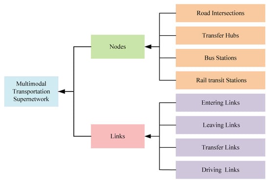
Figure 1.
The structure diagram of elements in the multimodal transportation super network.
2.2. Procedure of Establishing a Multimodal Super Network Topology
In this section, we present a multimodal transportation network that meets two requirements: one expresses the transfer among car, bus and rail transit modes; the other one shows the internal transfer of bus or rail transit mode. As shown in Figure 2, a traveler departs from the origin
to the destination . The transfer relationship among the transportation modes are described as follows: Firstly, passengers on bus line 2 can transfer to rail transit line 1 by transfer node 3, which represents the inter-modal transfer between bus and rail transit. Secondly, node 6 is the transfer station between bus line 2 and bus line 3, which stands for the inter-route transfer in the bus network. Moreover, passengers can drive from node 7 to node 10 and transfer to rail transit line 2 through the transfer link (9,10), which indicates the inter-modal transfer between car and rail transit. Besides, by the transfer node 12 passengers can transfer from rail transit line 1 to rail transit line 2, which shows the inter-route transfer in the rail transit network. Finally, all transfer nodes 3 → 3′, 6 → 6′, and 12 → 12′ are achieved by walking; and transfer links (9,10) and (16,17) are achieved by bike-sharing. Next, based on the super network theory, the process of establishing a multimodal transportation super network topology is as described in the following section.
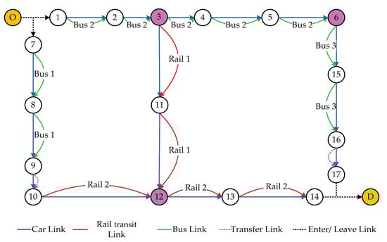
Figure 2.
The diagram of the multimodal transportation network.
2.2.1. Bus Network
The bus network is illustrated in Figure 3, which includes three bus routes, namely bus line 1, bus line 2, and bus line 3, where the pink node 6 is the transfer station. The information of routes in the bus network is shown in Table 2.
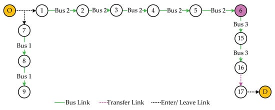
Figure 3.
The routes of the bus network.
Table 2.
The information of bus routes.
The transfer node 6 in Figure 3 can be extended to nodes 6 and 6′ through super network expansion, so Figure 3 becomes the bus super network topology, which is shown in Figure 4.
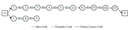
Figure 4.
The bus super network topology.
2.2.2. Rail Transit Network
The rail transit network is shown in Figure 5, which contains two rail transit routes, namely rail transit line 1 and rail transit line 2, where the pink node 12 is the transfer station. The information of routes in the rail transit network is shown in Table 3.
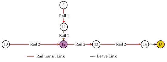
Figure 5.
The routes of the rail transit network.
Table 3.
The information of rail transit routes.
Like transfer node 6 discussed above, the transfer node 12 can be extended to nodes 12 and 12′ by super network expansion. As a result, the rail transit super network topology is as shown in Figure 6.
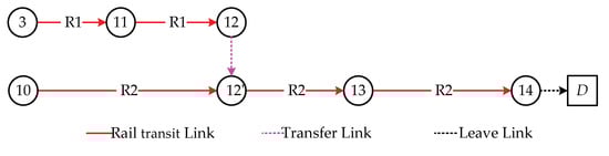
Figure 6.
The rail transit super network topology.
2.2.3. Car Network
The car network is shown in Figure 7. It contains three car routes, named car route 1, car route 2, and car route 3, respectively. The information of each route in the car network is shown in Table 4.
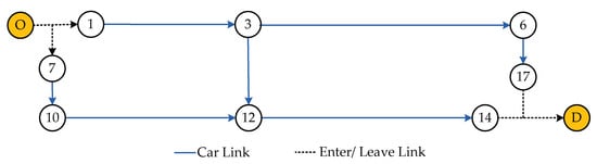
Figure 7.
The routes of the car network.
Table 4.
The information of car routes.
In general, for car mode passengers or drivers needn’t transfer in one trip, so it is unnecessary to expand nodes in the car network, the car super network topology is shown in Figure 8.
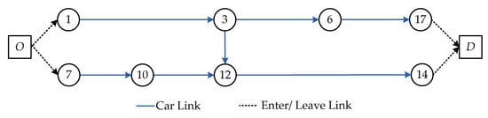
Figure 8.
The car super network topology.
In summary, by connecting the same nodes among different modes, a multimodal transportation super network topology (Figure 9) is obtained, of which three layers are bus, rail transit, and car network topology respectively. In Figure 9, the pink dotted links clearly illustrate the inter-modal transfers among bus, rail transit, and car, as well as the inter-route transfers of bus or rail transit.
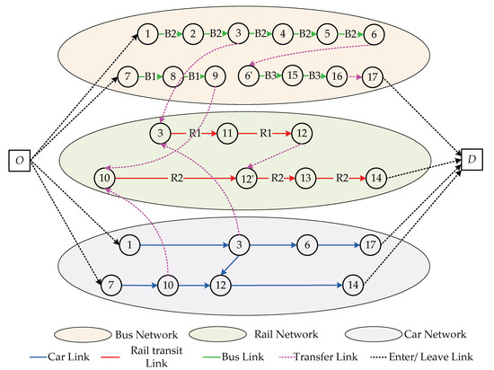
Figure 9.
The multimodal transportation super network topology.
3. Formulating the Multimodal Discrete Network Design Problem
In this section, firstly the generalized cost formulas of each type of links are defined. Then, a bi-objective programming optimization model of multimodal DNDP will be introduced.
3.1. The Generalized Cost Formula
Many factors affect the impedance of links in the multimodal networks. In this paper, the impact of travel time, monetary cost, and comfort are mainly considered. Among them, travel time includes walking time, driving time, and waiting time. Monetary cost can be divided into two types: mileage-based fare (such as the car mode) and route-based fare (such as the bus and rail transit mode).
The perception of comfort varies with the travel time due to different transportation modes. Besides, we reserve some time to prevent emergencies. Consequently, the generalized cost of links is mainly composed of travel time, monetary cost, and comfort loss, risk reserve time, which is specifically quantized as:
where : the weight coefficients and we have , : the travel time cost, : the corresponding time cost converted from currency conversion, : the corresponding time cost converted from the loss of comfort and : the reserved time for risk.
3.2. The Generalized Cost Formulas of Entering Links and Leaving Links
(1) Travel time
In the actual transportation system, entering links , indicate the process of reaching the stations, which mainly include walking time and waiting time; entering links , express the process of reaching the parking lot, which mostly includes walking time. Therefore, it can be concluded that the travel time of the entering links mainly consists of walking time and waiting time. Consequently, the travel time of the entering link can be formulated as:
where : the average walking time of the entering links and : the waiting time of the entering links. In this paper, it is set that , is the departure frequency, and .
Meanwhile, in the actual transportation system, leaving links () show the process of arriving at the destination, which mostly contains walking time. Hence, the travel time of the leaving links can be described as:
where is the average walking time of leaving links.
(2) Monetary cost
Since there is no monetary cost on the entering links and leaving links, we set the monetary cost to zero, which is formulated as:
where : the monetary cost of entering links and : the monetary cost of leaving links.
(3) Comfort loss
Since the trip is very short and the value of comfort loss is very small, we also set the comfort loss to zero on the entering links and leaving links. The equation is as follows:
where : the comfort loss of entering links and : the comfort loss of leaving links.
(4) Risk reserve time
According to travel time, so we set the risk reservation time of the entering links as:
where : the delay parameter of the entering links, and .
Similarly, the risk reservation time of the leaving links is formulated as:
where : the delay parameter of leaving links and .
3.3. The Generalized Cost Formulas of Driving Links
(1) Travel time
In the actual transportation system, driving links , , stand for the road between adjacent intersections. In this paper, we set the travel time of car driving links as:
where : the free-flow travel time, : the newly assigned traffic flow, : the original traffic flow, : the capacity of driving links, : the average number of passengers and ,: the undetermined coefficient.
Meanwhile, in the actual transportation system, driving links , indicate adjacent stations, and the travel time of the bus and rail transit driving links are set as:
where : the average travel time of the transportation mode .
(2) Monetary cost
Since the car is charged depending on mileages, in this paper, the monetary cost of the car driving links is described as:
where : the monetary cost per unit mileage,
: the length of the link .
Moreover, as the price of the ticket is up to mileages, the monetary cost of the bus and rail transit driving links are set as:
where : the starting fare, : the number of miles corresponding to the starting fare of the mode , : the length of the link and : the increasing ticket price per unit mileage.
(3) Comfort loss
As the comfort loss is proportional to the travel time on the car network, it can be formulated as:
where: : the degree of comfort loss per unit time of the car mode.
In addition, the comfort loss is mainly determined by travel time and congestion on the bus or rail transit network, so it can be described as:
where : the comfort loss parameter when the transportation mode is empty, : the comfort loss parameter when congestion occurs, : the number of passengers, : the departure frequency and : the capacity of vehicles.
(4) Risk reserve time
Similarly, we set the risk reservation time of the driving links as follows:
where : the delay parameter of driving links and .
3.4. The Generalized Cost Formulas of Transfer Links
(1) Travel time
It has been mentioned above that the transfer modes mainly consist of walking and bike-sharing. Therefore, the travel time of transferring to the transportation mode can be formulated as:
or:
where : the average walking time for transfer to the transportation mode , : the average cycling time for transfer to the transportation mode , : the waiting time for transfer to the transportation mode , and we set , is the departure frequency and .
(2) Monetary cost
Since there is no monetary cost for walking, and only the monetary cost of bike-sharing exists, the monetary cost of transferring to the mode can be represented as:
or:
where : the starting fare for cycling, : the number of miles corresponding to the starting fare for cycling, : the length of the link and : the increasing fare per unit mileage.
(3) Comfort loss
Since the transfer trip is very short and the comfort loss can be ignored, we set the comfort loss of transferring to the transportation mode as:
(4) Risk reserve time
Similarly, the risk reservation time of transferring to the transportation mode is expressed as:
where : the delay parameter of transferring to the transportation mode and .
3.5. Bi-Objective Programming Model
The objective of multimodal DNDP is to decide on an optimal scheme from the candidate schemes to minimize the total cost, which includes the network operation cost and the construction cost of the optimization scheme. is the set of candidate links; is the set of added or expanded links for the car network; is the set of added or expanded links for the rail transit network, and is the set of added or expanded links for the bus network.
(1) Network operation cost
According to the generalized cost formulas mentioned above, the network operation cost of the multimodal transportation network can be formulated as follows:
Here, is the traffic flow of the link .
(2) Construction cost
For DNDP, there are two methods to optimize the network: one is to add a new link; the other one is to expand the original link. In the multimodal super network topology, an added link is to connect two unconnected nodes, while an expanded link is to add a link to the originally connected nodes.
As shown in Figure 10: for the car network, since node 3 and node 14 were not connected originally, the added link (3,14) (the blue dotted link) represents the added optimization. Meanwhile, as node 7 and node 10 were connected originally, so link (7,10) (the blue dotted link) illustrates the expanded optimization. Therefore, we use the 0-1 variable and to respectively express whether to add or expand links. If the link is added/expanded, is equal to 1, otherwise is equal to 0,
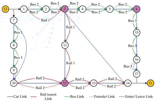
Figure 10.
The diagram of optimization schemes.
For the bus network, the added method indicates adding a new link on the existed route, like link (16,17) (the green dotted link). The expanded method means to increase the frequency of departure, so it will change the whole route, such as link (1,2), (2,3), (3,4), (4,5), (5,6) (the green dotted link). Hence, if the link is added/expanded the 0–1 variable is equal to 1, otherwise is equal to 0, in the bus network.
Similarly, for the rail transit network, the added method expresses to add a new link on the existed route, like link (1,3) (the red dotted link). And the expanded method represents to increase the frequency of departure, so it will change the whole route, such as links (10,12), (12,13), (13,14) (the red dotted link). Thus, if the link is added/expanded the 0–1 variable is equal to 1, otherwise is equal to 0, in the rail transit network.
Consequently, the construction cost of the optimization scheme is formulated as:
where : the cost of the added link for the mode and : the cost of the expanded link for the mode .
(3) Bi-objective programming model
In summary, a bi-objective programming model for multimodal DNDP is proposed based on Equations (21) and (22) to minimize the network operation cost and construction cost as follows:
where , : the weight coefficients and we have , : the budget cost of the transportation mode , ,: the original traffic flow and the original capacity of the link respectively, : the traffic demand of OD pair , : the capacity of the added/expanded link for the mode ,: the binary variable, if the link is expanded, is equal to 1, otherwise, is equal to 0 on the bus or rail transit route and : the number of expanded links on the bus or rail transit route.
Constraints (24)–(26) indicate that the cost of optimization schemes is less than the budget cost for car, bus, and rail transit network.
Constraint (27) shows that the sum of the assigned traffic flow and the original traffic flow is less than the sum of the original capacity and the increased capacity of the added or expanded optimization.
Constraints (28)–(31) are traffic flow equilibrium constraints, where constraint (28) means that for the starting point, the outflow minus the inflow is equal to . Constraint (29) shows that for the destination point, the outflow minus the inflow is equal to . Constraint (30) expresses that for each node, the outflow and inflow must be equal. Constraint (31) indicates that the traffic flow cannot be less than zero.
Constraint (32) ensures that the expanded method will change the whole existed route for the bus and rail transit network. Specifically, if one link of the route is expanded, then the other links must be expanded.
4. Solution Algorithm
Since there are two types of decision variables in the proposed optimization model: the assignment of traffic flow and the decision of adding or expanding candidate links, the algorithm is divided into two parts:
Firstly, we need to assign the traffic flow to minimize the network operation cost. Since the capacity of each link is considered in the proposed model, it is appropriate that the minimum cost flow algorithm is applied to solve this problem.
Secondly, as multimodal DNDP is an integrated optimization problem, conventional solving algorithms are difficult to solve efficiently, heuristic algorithms are developed in this paper: simulated annealing algorithm to search the near-optimal decision from the candidate schemes .
4.1. Minimum Cost Flow Algorithm
Let be the minimum cost augmentation chain of the -th iteration, be the adjustable flow on the augmentation chain , and be the feasible flow of the -th iteration. Based on the shortest path method, a network is constructed, whose nodes are the nodes of the original network , specifically, the link of the original network is changed into two links with opposite directions and . Define the weights of links and in as and :
Set the matrix , represents the shortest length from to in the original network ; , represents the end number of the first link of the shortest path from to . For example, if , the first link of the shortest path from to is .
Above all, the algorithm for solving the minimum cost feasible flow with the target flow is as follows:
Step 1: Set = 0
Start with a minimum cost initial feasible flow (generally, ).
Step 2: Generate , find the minimum cost path from to in , and use the Floyd algorithm to solve the shortest path.
Step 2.1: Set
Step 2.2:
Calculate:
where:
If go to step 2.2, else go to step 2.3.
Step 2.3: when , the algorithm ends.
, is the shortest path length from to ;
, is the end node of the first link in the shortest path from to .
Step 3: If does not have the shortest path from to , then is regarded as the maximum flow, there is no minimum cost flow with the target flow of , end the algorithm; otherwise, go to the next step.
Step 4: Find the augmented chain corresponding to the shortest path from to in in the original network , and calculate . If , according to the maximum flow adjustment scheme, adjust the augmented flow on the augmented chain to obtain a new flow , and let , assign new flow to , go to step 2; otherwise, when , adjust the augmented flow on the augmented chain to obtain a new flow , where is the minimum feasible flow of the target flow . End the algorithm.
4.2. Simulated Annealing Algorithm
(1) Determination of solution space
In this problem, all the possible added and expanded candidate schemes constitute the solution space, and a specific candidate scheme can be regarded as a partition of the set , where , , and or is the feasible solution. The solution space is composed of all possible partitions, that is
(2) Objective formula
According to the discussion presented in Section 3.5, the objective function of the optimization schemes can be defined as:
(3) The choice of initial solution
The initial solution is the initial point of the simulated annealing algorithm. A large number of experiments show that the final solution of the simulated annealing algorithm does not depend on the selection of the initial solution, so we randomly choose an initial as .
(4) The generation of a new solution
For this algorithm, we first need to use a certain strategy to generate a new solution based on the current solution in the space, then decide whether to accept the new solution. When the new solution is accepted, which will be treated as a new current solution, and the value of the objective function is modified correspondingly. The next iteration is started on this basis. If the new solution is not accepted, the next experiment will be continued based on the current solution.
Since the proposed optimization model is a binary integer programming, we can arbitrarily choose . If is 0, it will be replaced by 1; otherwise, if it is 1, it will be replaced by 0. Therefore, a new solution is generated and the difference of values of the objective function in two iterations can be calculated by the following formula:
(5) Acceptance criterion
An acceptance criterion is set to judge whether the new solution is accepted or not. Generally, the most commonly used acceptance criteria is Metropolis criteria:
where is the control parameter.
According to the settings above, the procedure of the simulated annealing algorithm is listed as follows:
Step 1: Randomly select an initial solution , let the current solution ; the current number of iteration steps ; the current temperature .
Step 2: When reaching the maximum number of iterations the inner loop, go to step 3; otherwise, randomly select a neighbor from the neighborhood and calculate , if then , otherwise, if (represents a uniform random number between 0 and 1), then , repeat step 2.
Step 3: (representing the formula of temperature drop), and the classic simulated annealing algorithm cooling formula is . If the end temperature , is reached, go to Step 4, otherwise, go to Step 2.
Step 4: Output the calculation result and stop.
As shown in Figure 11, the simulated annealing algorithm includes an inner loop and an outer loop. The inner loop is the second step, which means random search in the neighborhood at the same temperature . The outer loop mainly includes the temperature drop change , the number of iteration steps , and the stop condition in the third step.
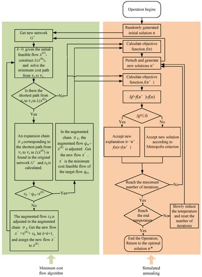
Figure 11.
The flow chart of the multimodal DNDP solution algorithm.
Consequently, we combine the minimum cost flow algorithm and simulated annealing algorithm as a hybrid heuristic algorithm that can solve the proposed model. The relationship between the minimum cost flow algorithm and the simulated annealing algorithm is shown in Figure 11. The minimum cost flow algorithm will be used to assign traffic flow before solving the objective function in each iteration of the simulated annealing algorithm.
5. Numerical Examples
In this section, two numerical tests are implemented to validate the proposed model and algorithm: a simple test network (the multimodal transportation network shown in Figure 2) and an actual network (an area of Beijing, China). All experiments are executed in Python software on a Lenovo laptop configured with an Intel Core i5-8250U 3.40 GHz CPU equipped with 8 GB RAM.
5.1. Simple Network
Before optimization, the maximum feasible flow of the network is 78, and the traffic demand is 100, so it is necessary to improve the network. According to the passenger demand, some candidate links are given, as shown in Figure 12: the blue dotted links (3,14), (7,10) are the candidate links for the car network, namely ={(3,14), (7,10)}; the green dotted link (16,17) is the candidate link for the bus network, namely ={(16,17)}; the red dotted link (1,3) is the candidate link for the rail transit network, namely ={(1,3)}. Therefore, it can be concluded that the set of candidate schemes = {(3,14), (7,10), (16,17), (1,3)}, so there are in total 24 schemes. Next, we will use the exact algorithm and heuristic algorithm respectively to find the near-optimal scheme from the 24 schemes.
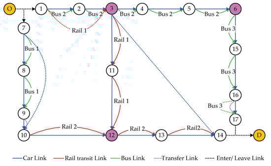
Figure 12.
The optimization schemes on a simple multimodal network.
(1) Exact algorithm
To test the feasibility of the developed heuristic algorithm, an exact algorithm is first used to solve the model. The specific steps are as follows:
Step 1: Calculate the generalized cost of each type of links
Firstly, give the information of links for each network in the multimodal transportation, among which, the car network mainly includes length (km), zero traffic flow driving time (min), existing vehicle (pcu/h), capacity (pcu/h); the bus network and rail transit network mainly include average driving time (min), frequency (number/ hour); transfer network mainly includes length (km), walking time (min) and cycling time (min). Then, calculate the generalized cost of each type of links according to the formulas in Section 3, and the results are shown in Figure 13: in brackets, the first term is the generalized cost of links and the second term is the capacity of links.
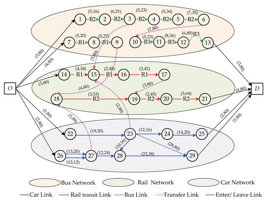
Figure 13.
The generalized cost and capacity of each link in the super network topology.
As shown in Figure 13: in the multimodal transportation super network topology, the blue dotted links (26,27) and (23,29) respectively represent the candidate links (3,14), (7,10) (in Figure 12) for the car network; the red dotted link (14,15) stands for the candidate link (1,3) (in Figure 12) for the rail transit network, and the green dotted link (12,13) expresses the candidate link (16,17) (in Figure 12) for the bus network.
Step 2: Traffic flow assignment
The minimum cost flow algorithm is coded by PYTHON based on the steps in Section 4.1 to assign the traffic flow. The traffic flow assignment and the composition of transportation mode for each shortest path are obtained, as shown in Table 5, in which all candidate links are taken.
Table 5.
The traffic flow assignment and composition of transportation mode for the shortest path.
Step 3: Calculate the value of the objective function
The optimal result of traffic flow assignment in step 2 is used to calculate the value of the network operation cost by Equation (21); then based on the optimization cost and the budget cost of each candidate link to calculate the value of construction cost by Equation (22); finally, the weighted sum of the operation cost and the construction cost by Equation (23) is the value of the objective function. When the generalized cost formula coefficients = 0.25,= 0.25, = 0.25, 0.25 in Equation (1), and the objective function weight coefficients 0.5, 0.5 in Equation (23), the calculation results are illustrated in Table 6 and Figure 14.
Table 6.
Optimization results of the exact algorithm.
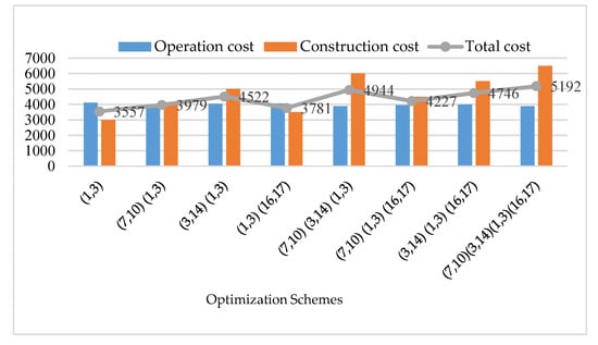
Figure 14.
The optimization results of the exact algorithm.
It can be concluded from Table 6 and Figure 14 that the optimal solution of the exact algorithm is (1,3), and the corresponding operation cost is 4114, construction cost is 3000, and total cost is 3557. Some schemes are without values of construction cost and objective function in Table 6. Because the maximum feasible flow of the schemes does not reach = 100, so the optimization schemes are not adopted, and there is no need to calculate the objective function.
(2) Heuristic algorithm
Similarly, the developed heuristic algorithm is also coded by PYTHON based on the steps in Section 4.2 to solve the model, and we set the initial temperature = 500, the end temperature = 100, the maximum number of iterations = 50. Besides, according to Equation (43), the relative error between the heuristic algorithm and the exact algorithm is calculated. The results are shown in Table 7.
GAP= (near-optimal solution − exact solution)/exact solution × 100%
Table 7.
Comparison between the heuristic algorithm and the exact algorithm.
Clearly, the solution calculated by the heuristic algorithm is the same as the exact algorithm, which verifies the effectiveness and feasibility of the heuristic algorithm. To further test the heuristic algorithm, then we carry out sensitivity analysis of parameters in Equations (1) and (23).
(3) Sensitivity analysis
In this section, the sensitivity analysis is carried out on the weight coefficients of the generalized cost formula Equation (1) and the weight coefficients of the objective formula Equation (23) . The specific results are listed in Table 8.
Table 8.
Comparison between heuristic and exact algorithm under different weight coefficients.
It can be seen from Table 8 that the results obtained by the heuristic algorithm are basically consistent with the exact solution, and only two calculation results deviate from the exact value. Moreover, the relative errors of the two results obtained by the two algorithms are within 1.5%, which validates the effectiveness and reliability of the heuristic algorithm within the allowable error range. In addition, the exact algorithm takes several hours to obtain the optimal solution, while the heuristic algorithm takes only within 56 s. Therefore, the heuristic algorithm is superior to the exact solution algorithm in terms of calculation time.
5.2. Actual Network
The actual transportation network in this case is an area from Xizhimen to Dongdan in Beijing, China. It is one of the busiest traffic areas in Beijing. The network of this area includes multiple bus, rail transit lines and integrates various travel modes, such as car, rail transit, bus, bicycle, and walking. It has many important transfer hub stations. So it is a typical multimodal transportation network. Moreover, there are many facilities for sharing bicycles near each transfer station, which facilitates passengers’ transfer behavior. That is consistent with the model proposed in this paper, which takes bike-sharing as a transfer mode. In addition, due to the huge passenger demand from Xizhimen to Dongdan and the bottleneck of the transportation network, the network capacity is insufficient. Thus, it is necessary to expand or add some links for the car, bus, and rail networks respectively. This is also an important reason why this regional network is selected as an actual case. The multimodal transportation network diagram is as follows, which combined car, bus, and rail transit modes.
As shown in Figure 15: the origin is Xizhimen while the destination is Dongdan. The transfer relationship among modes is as follows, among them, the pink nodes are the transfer stations:
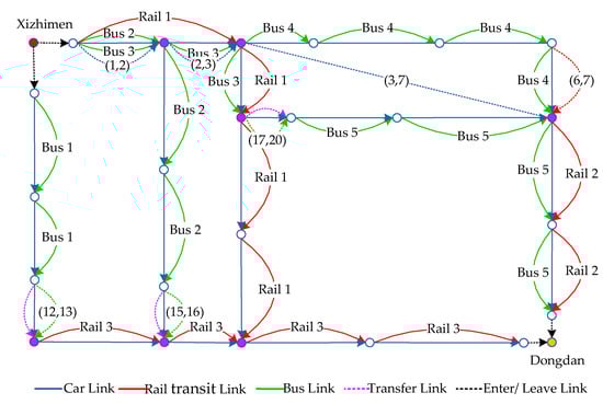
Figure 15.
Multimodal transportation network from Xizhimen to Dongdan.
- Firstly, inter-modal transfers between bus and rail transit include 3 routes: (1) bus line 1 → rail line 3; (2) bus line 2 → rail line 3; (3) bus line 3→ bus line 4 → rail line 2.
- Secondly, the inter-route transfers in the bus network include 2 routes: (1) bus line 3 → bus line 5; (2) bus line 3 → bus line 4 → bus line 5.
- Moreover, the inter-route transfer in the rail transit network only includes 1 route: rail line 2 → rail line 3.
- Besides, the inter-modal transfer between car and rail transit includes 1 route: passengers drive from the origin Xizhimen to node 13 and transfer to rail line 3 by node 13.
Before optimization, the maximum feasible flow of the network is 1524, and the traffic demand is 2000, so it is necessary to improve the network. According to the passenger demand, the candidate links are given, as shown by the dotted line in Figure 15: for the car network, the blue dotted links (1,2), (2,3) represent the expansion optimization, and the blue dotted link (3,7) is the candidate link for the adding optimization, namely ={(1,2), (2,3), (3,7)}; for the bus network, the green dotted links (12,13), (15,16), (17,20) are the candidate links for adding optimization, namely ={(12,13), (15,16), (17,20)}; for the rail transit network, the red dotted link (6,7) is the candidate link for adding optimization, namely = {(6,7)}. Therefore, it can be concluded that the set of candidate schemes = {(1,2), (2,3), (3,7), (12,13), (15,16), (17,20), (6,7)}, so there are totally 27 schemes. Next, we use the heuristic algorithm to find the near-optimal scheme from the 27 schemes.
The multimodal transportation super network topology is built and the link information of each network is given to calculate the generalized cost of each type of links, as shown in Figure 16: in brackets, the first term is the generalized cost of links and the second term is capacity of links.
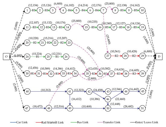
Figure 16.
The generalized cots and capacity of each link in the super network topology.
Finally, the proposed heuristic algorithm will be coded by PYTHON for the numerical test based on Section 4, which combines the minimum cost flow algorithm and simulated annealing algorithm. And we set the initial temperature = 1000, the end temperature = 100, the maximum number of iterations = 200. To analyze the optimal schemes under different weight coefficients, 12 groups of numerical experiments are carried out. The near-optimal schemes under different weight coefficients are shown in the table below.
It can be concluded from Table 9 that the choice of the near-optimal scheme is affected by the weight coefficients:
Table 9.
Optimization results of the actual network under different weight coefficients.
- (1)
- When the value of is larger than in Equation (1), the travel time is the main priority, and passengers are more willing to choose the car mode that can reach the destination quickly. In this case, when = 0.6 (group 8,9,10), the car’s candidate links (1,2), (2,3) are all adopted in various groups, which are consistent with the choice of passengers. On the contrary, the monetary cost is focused on, and passengers prefer to choose the transportation mode that can save a lot of money. While = 0.6 (group 11,12,13), the bus’s candidate links (12,13), (15,16), (17,20) are all adopted in various groups, which are also tally with the actual situation
- (2)
- When the value of is larger than in Equation (23), the decision-maker pays more attention to the network operation cost. In this case, when = 0.9 (group 2,5,8,11), the car’s candidate links (1,2), (2,3) are the principal part of the near-optimal scheme under different groups. Conversely, the construction cost is mainly considered. While = 0.9 (group 3,6,9,12), the bus’s candidate links (12,13), (15,16), (17,20) are the main component of the near-optimal scheme in various groups. These are consistent with the actual situation, which proves that the developed heuristic algorithm can efficiently find the near-optimal solution with good stability and reliability.
Therefore, in an actual operation situation, the value of each parameter can be set according to the attention of the decision-maker, for example, when the travel time is more important, the value of is larger than , otherwise, the monetary cost is mainly considered; when decision-maker pays more attention to the operation cost, the value of is larger than , conversely, the construction cost is principal considered.
Consequently, the good results of the two numerical tests are obtained in this section, which shows that the proposed model and developed algorithm in this paper are feasible and efficient.
6. Conclusions
In this paper, we comprehensively optimize a multimodal transportation DNDP that is composed of car, bus, rail transit, bicycle, and walking. Firstly, a multimodal super network topology that includes four types of links (entering links, leaving links, driving links, transfer links) is proposed, which clearly expresses inter-modal transfers among car, bus, and rail transit networks, as well as inter-route transfers in the bus or rail transit network. And to complete the above transfers, walking and bike-sharing are considered as transfer modes. Specifically, in Section 2 we present a simple multimodal transportation network that meets two types of the above transfer relationships and we also discuss the process of establishing a multimodal transportation super network topology. Secondly, the generalized cost formulas of each type of links in the super network topology are defined. Among them, the generalized cost is mainly composed of four types, namely travel time, monetary cost, and comfort loss, risk reserve time. Based on the above formulas, a bi-objective programming model to minimize the network operation cost and construction cost is proposed to decide whether to expand or add links for the car, bus, and rail network respectively. Moreover, based on the minimum cost flow algorithm and simulated annealing algorithm, we develop a hybrid heuristic algorithm to solve the proposed model, which can efficiently and effectively get the near-optimal solution. Finally, two numerical tests of a simple test network (designed in Section 2) and an actual network (an area from Xizhimen to Dongdan in Beijing, China) are implemented:
- (1)
- For the simple network, to test the feasibility of the developed heuristic algorithm, an exact algorithm is first used to solve the model. And the results show that the proposed algorithm is effective and feasible within the allowable error range of 1.5%.
- (2)
- For the actual network, 12 groups of numerical experiments are carried out to analyze the optimal schemes under different weight coefficients. The results indicate that the choice of the near-optimal scheme is affected by the weight coefficients, and the results are consistent with the actual situation, Consequently, the proposed model and developed algorithm can promote the planning of multimodal transportation systems in the actual transportation network.
In this paper, the proposed model and developed algorithm are flexible, and the objective function and constraints can be modified. In our future works, we can consider the network accessibility, environmental pollution, and other aspects, and modify the objective function and constraints correspondingly. In addition, the algorithm can be combined with other heuristic algorithms, such as tabu search algorithm, genetic algorithm, and so on, to get the near-optimal solution more quickly.
The study of multimodal transportation DNDP is conductive to guide passengers’ multimodal travel behavior and relieve congestion. The practical implications are as follows: (1) By studying the multimodal transportation DNDP, the optimal investment scheme of transportation network planning and construction can be obtained to provide comparison and reference for traffic planning departments, decision-makers, and researchers. (2) In the complicated urban transportation network formed by various modes, grasping the mutual influence between the operation of the multimodal transportation networks as a whole is helpful to improve the level of transportation management measures, and also conducive to giving full play to the advantages of various modes and coordinate the combination of various modes. These will bring great improvement to the transportation congestion, thus reducing vehicle delays and transportation costs.
Certain disadvantages of the proposed methods need to be mentioned here. In this paper, only single OD is considered, and the passenger demand is determined. In future work, we will study the multimodal DNDP of multi-OD under uncertain demand. In addition, this paper only studies five representative travel modes: car, bus, and rail transit, walking, and bike-sharing. However, they can be subdivided into many types in real life. For example, the car model includes private cars, taxis, online car-hailing, etc. And electromobile, motorcycle and so on are also the travel modes that many people choose. Therefore, we can take these into account to improve the proposed model in future work.
Author Contributions
Conceptualization, C.C. and Y.Z.; methodology, Y.Z.; software, Z.F.; validation, Y.Z., C.C. and Z.F.; formal analysis, Y.Z.; investigation, Y.Z.; resources, C.C.; data curation, Y.Z.; writing—original draft preparation, Y.Z.; writing—review and editing, Z.F.; visualization, Y.Z.; supervision, C.C.; project administration, C.C.; funding acquisition, C.C. All authors have read and agreed to the published version of the manuscript.
Funding
This research was funded by Research Foundation of State Key Laboratory of Rail Traffic Control and Safety, Beijing Jiaotong University, China (RCS2021ZZ002).
Institutional Review Board Statement
This study did not involve humans or animals.
Informed Consent Statement
This study did not involve humans or animals.
Data Availability Statement
This study did not report any data.
Conflicts of Interest
The authors declare no conflict of interest.
References
- Sheffi, Y. Urban Transportation Networks: Equilibrium Analysis with Mathematical Programming Methods; Prentice-Hall: Hoboken, NJ, USA, 1984; pp. 231–261. [Google Scholar]
- Nagurney, A.; Dong, J. Supernetworks: Decision-Making for the Information Age; Edward Elgar Publishers: Chelthenham, UK, 2002; pp. 803–818. [Google Scholar]
- Frank, H.P.; Myrna, H.W. Networks and farsighted stability. Econ. Theory 2005, 120, 257–269. [Google Scholar]
- Daniele, P.; Maugeri, A.; Oettli, W. Time-Dependent Traffic Equilibria. Optim. Theory Appl. 1999, 103, 543–555. [Google Scholar] [CrossRef]
- Yamada, T.; Imai, K.; Nakamura, T.; Taniguchi, E. A supply chain–transport supernetwork equilibrium model with the behaviour of freight carriers. Transp. Res. Part E 2011, 47, 887–907. [Google Scholar] [CrossRef]
- Yamada, T.; Febri, Z. Freight transport network design using particle swarm optimisation in supply chain–transport supernetwork equilibrium. Transp. Res. Part E 2015, 75, 164–187. [Google Scholar] [CrossRef]
- Feng, Z.; Wang, Z.; Chen, Y. The equilibrium of closed-loop supply chain supernetwork with time-dependent parameters. Transp. Res. Part E 2014, 64, 1–11. [Google Scholar] [CrossRef]
- Chen, H. A Heuristic Solution Algorithm for the Combined Model of the Four Travel Choices with Variable Demand. East Asia Soc. Transp. Stud. 2015, 11, 326–341. [Google Scholar]
- Abdulaal, M.; Leblanc, L.J. Continuous equilibrium network design models. Transp. Res. Part B 1979, 13, 19–32. [Google Scholar] [CrossRef]
- Marcotte, P.; Marquis, G. Efficient implementation of heuristics for the continuous network design problem. Ann. Oper. Res. 1992, 34, 163–176. [Google Scholar] [CrossRef]
- Ban, J.X.; Liu, H.X.; Ferris, M.C.; Bin, R. A general MPCC model and its solution algorithm for continuous network design problem. Math. Comput. Model. 2006, 43, 493–505. [Google Scholar] [CrossRef]
- Chiou, S.W. A subgradient optimization model for continuous road network design problem. Appl. Math. Model. 2009, 33, 1386–1396. [Google Scholar] [CrossRef]
- Li, C.; Yang, H.; Zhu, D.; Meng, Q. A global optimization method for continuous network design problems. Transp. Res. Part B 2012, 46, 1144–1158. [Google Scholar] [CrossRef]
- LeBlanc, L.J. An algorithm for the discrete network design problem. Transp. Sci. 1975, 9, 183–199. [Google Scholar] [CrossRef]
- Farvaresh, H.; Sepehri, M.M. A single-level mixed integer linear formula for a bi-level discrete network design problem. Transp. Res. Part E 2011, 47, 623–640. [Google Scholar] [CrossRef]
- Poorzahedy, H.; Turnquist, M.A. Approximate algorithms for the discrete network design problem. Transp. Res. Part B 1982, 16, 45–55. [Google Scholar] [CrossRef]
- Gao, Z.; Wu, J.; Sun, H. Solution algorithm for the bi-level discrete network design problem. Transp. Res. Part B 2005, 39, 479–495. [Google Scholar] [CrossRef]
- Wang, S.; Meng, Q.; Yang, H. Global optimization methods for the discrete network design problem. Transp. Res. Part B 2013, 50, 42–60. [Google Scholar] [CrossRef]
- Wang, Z.W.D.; Liu, H.; Szeto, W.Y. A novel discrete network design problem formula and its global optimization solution algorithm. Transp. Res. Part E 2015, 79, 213–230. [Google Scholar] [CrossRef]
- Di, Z.; Yang, L. Reversible lane network design for maximizing the coupling measure between demand structure and network structure. Transp. Res. Part E 2020, 41, 102021. [Google Scholar] [CrossRef]
- Wan, Q.K.; Lo, H.K. A mixed integer formulation for multiple-route transit network design. Math. Modell. Algorithms 2003, 2, 299–308. [Google Scholar] [CrossRef]
- Baaj, M.H.; Mahmassani, H.S. An AI-based approach for transit route system planning and design. Adv. Transp. 1991, 25, 187–210. [Google Scholar] [CrossRef]
- Mauttone, A.; Urquhart, M.E. A route set construction algorithm for the transit network design problem. Comput. Oper. Res. 2009, 36, 2440–2449. [Google Scholar] [CrossRef]
- Yang, Z.; Yu, B.; Cheng, C. A parallel ant colony algorithm for bus network optimization. Comput. Aided Civil Environ. Eng. 2007, 22, 44–55. [Google Scholar] [CrossRef]
- Yu, B.; Yang, Z.; Jin, P.; Wu, S.; Yao, B. Transit route network design-maximizing direct and transfer demand density. Transp. Res. Part C 2012, 22, 58–75. [Google Scholar] [CrossRef]
- Yao, B.; Hu, P.; Lu, X.; Gao, J.; Zhang, M. Transit network design based on travel time reliability. Transp. Res. Part C 2014, 43, 233–248. [Google Scholar] [CrossRef]
- Amirgholy, M.A.; Shahabi, M.; Gao, H. Optimal design of sustainable transit systems in congested urban networks: A macroscopic approach. Transp. Res. Part E 2017, 103, 261–285. [Google Scholar] [CrossRef]
- Chen, J.; Liu, Z.; Wang, S.; Chen, X. Continuum approximation modeling of transit network design considering local route service and short-turn strategy. Transp. Res. Part E 2018, 119, 165–188. [Google Scholar] [CrossRef]
- Feng, X.; Zhang, J.; Chen, J.; Wang, G.; Zhang, L.; Li, R. Design of Intelligent Bus Positioning Based on Internet of Things for Smart Campus. IEEE Access 2018, 6, 6005–6015. [Google Scholar] [CrossRef]
- Wan, Q.K.; Lo, H.K. Congested multimodal transit network design. Publ. Transp. 2009, 1, 233–251. [Google Scholar] [CrossRef]
- Uchida, K.; Sumalee, A.; Watling, D.; Connors, R. A study on network design problems for multi-modal networks by probit-based stochastic user equilibrium. Netw. Spat. Econ. 2007, 7, 213–240. [Google Scholar] [CrossRef]
- Li, X.; Luo, Y.; Wang, T.; Kuang, H. An integrated approach for optimizing bi-modal transit networks fed by shared bikes. Transp. Res. Part E 2020, 141, 102016. [Google Scholar] [CrossRef]
- Gallo, M.; D’acierno, L.; Montella, B. A Meta-heuristic Algorithm for Solving the Road Network Design Problem in Regional Contexts. Procedia-Soc. Behav. Sci. 2012, 54, 84–95. [Google Scholar] [CrossRef][Green Version]
- Zhang, L.; Yang, H.; Wu, D.; Wang, D. Solving a discrete multimodal transportation network design problem. Transp. Res. Part C 2014, 49, 73–86. [Google Scholar] [CrossRef]
- Cai, X.; Pei, Y. Review of the Cycling Network Planning and Design in Chinese Cold-Climate Cities. IEEE Access 2017, 1–23. [Google Scholar] [CrossRef]
- Liu, H.; Szeto, W.Y.; Long, J. Bike network design problem with a path-size logit-based equilibrium constraint: Formulation, global optimization, and matheuristic. Transp. Res. Part E 2019, 127, 284–307. [Google Scholar] [CrossRef]
Publisher’s Note: MDPI stays neutral with regard to jurisdictional claims in published maps and institutional affiliations. |
© 2021 by the authors. Licensee MDPI, Basel, Switzerland. This article is an open access article distributed under the terms and conditions of the Creative Commons Attribution (CC BY) license (https://creativecommons.org/licenses/by/4.0/).