A Hybrid Bat Algorithm for Solving the Three-Stage Distributed Assembly Permutation Flowshop Scheduling Problem

Abstract

In this paper, a hybrid bat optimization algorithm based on variable neighbourhood structure and two learning strategies is proposed to solve a three-stage distributed assembly permutation flowshop scheduling problem to minimize the makespan. The algorithm is firstly designed to increase the population diversity by classifying the populations, which solves the difficult trade-off between convergence and diversity of the bat algorithm. Secondly, a selection mechanism is used to update the bat’s velocity and location, solving the difficulty of the algorithm to trade-off exploration and mining capacity. Finally, the Gaussian learning strategy and elite learning strategy assist the whole population to jump out of the local optimal frontier. The simulation results demonstrate that the algorithm proposed in this paper can well solve the DAPFSP. In addition, compared with other metaheuristic algorithms, IHBA has better performance and gives full play to its advantage of finding optimal solutions.

1. Introduction

The distributed assembly scheduling problem is a derivative and extension of the assembly scheduling problems. It is mainly used to produce multiple products assembled from different parts. In a decentralized and globalized economy, the current economic trend of customization and intelligent manufacturing has led to the rapid development of assembly production. Internationally, international companies with multiple production centers or plants are even more common. This shows that distributed and intelligent production plays a pivotal and irreplaceable role in the modern manufacturing industry. Currently, this type of scheduling is widely used in the supply chain and manufacturing industry. In order to maintain a competitive position in a rapidly changing market, managers must quickly make the right decisions about how to allocate work to plants and how to schedule each plant efficiently. Therefore, the distributed scheduling problem has become a hot research topic among scholars and researchers.

The distributed assembly permutation flowshop scheduling problem (DAPFSP) is of great importance to both the industrial industry and the research community. As we all know, DAPFSP consists of two phases, including production and assembly. In detail, the production phase corresponds to a distributed displacement flowshop scheduling problem, where n jobs are assigned to be processed in f plants with m identical machines in a flowshop line. Each job belongs to a certain product. The processes contained in each product cannot be interrupted or inserted by processes of other products during the production process. The assembly phase corresponds to the assembly flow shop scheduling problem, where s products are made in an assembly plant with a single assembly machine, and each product must be assembled after all processes produced in the production phase are completed.

Total completion time has been identified as a more relevant and meaningful goal in today’s dynamic manufacturing environment when a batch of work needs to be completed as quickly as possible. This allows the objective function to minimize the flow of work and efficiently improve resource utilization. DPFSP is an NP-hard with m greater than or equal to 2, and is a derivation and extension of the traditional permutation flow shop scheduling problem with this criterion. Similarly, DAPFSP can be seen as an extension of DPFSP, which is more complex than DPFSP. Therefore, the DAPFSP with completion time as the objective function is also a strong NP-hard problem. In recent years, as a simple yet efficient method, the bat algorithm has solved many scheduling problems in academia, including the job shop scheduling problem [1], the open shop scheduling problem [2], the task scheduling problem [3], and the production scheduling problem [4], by continuously performing local search in the neighborhood of the current solution to obtain the optimal solution.

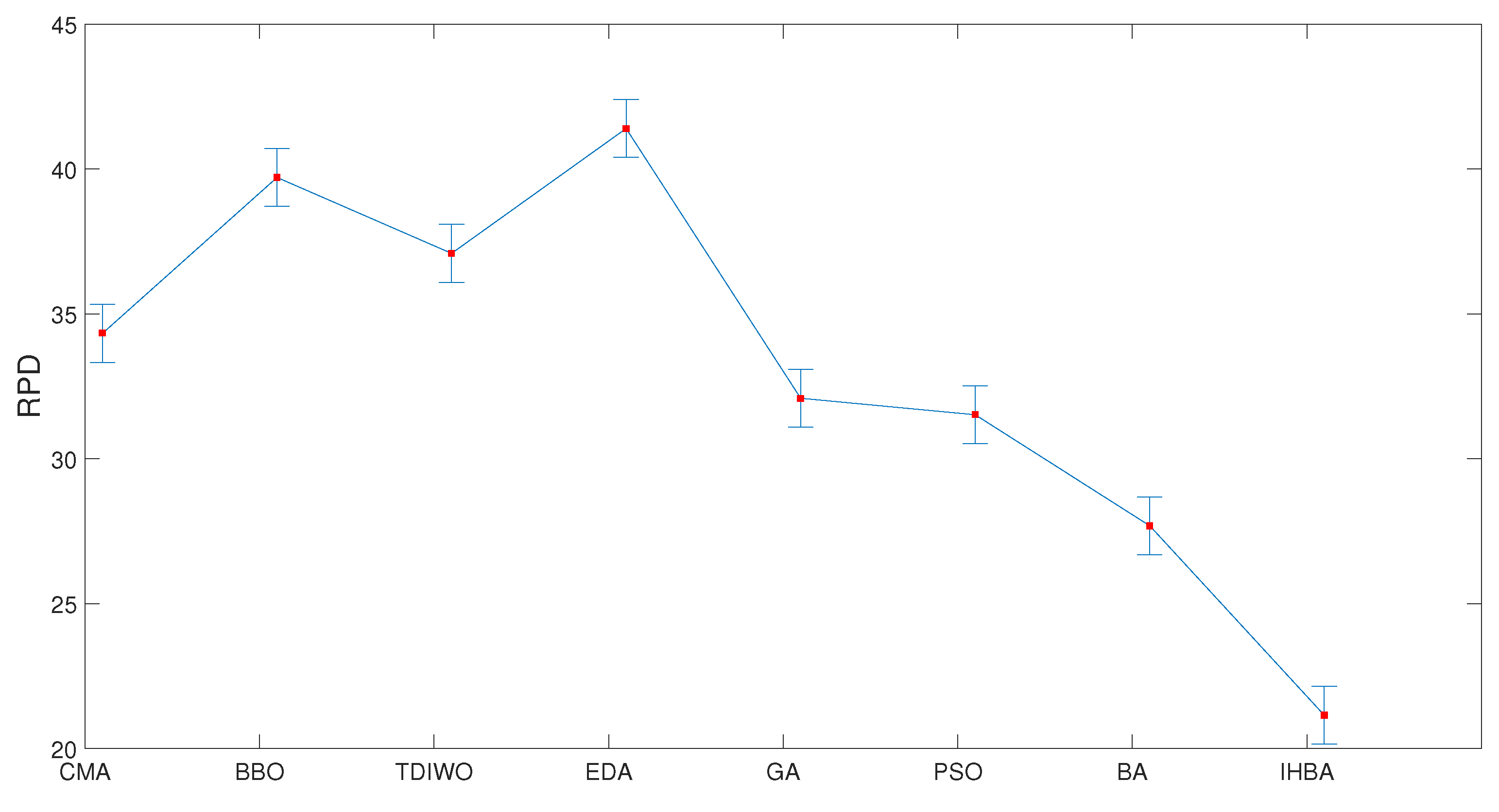
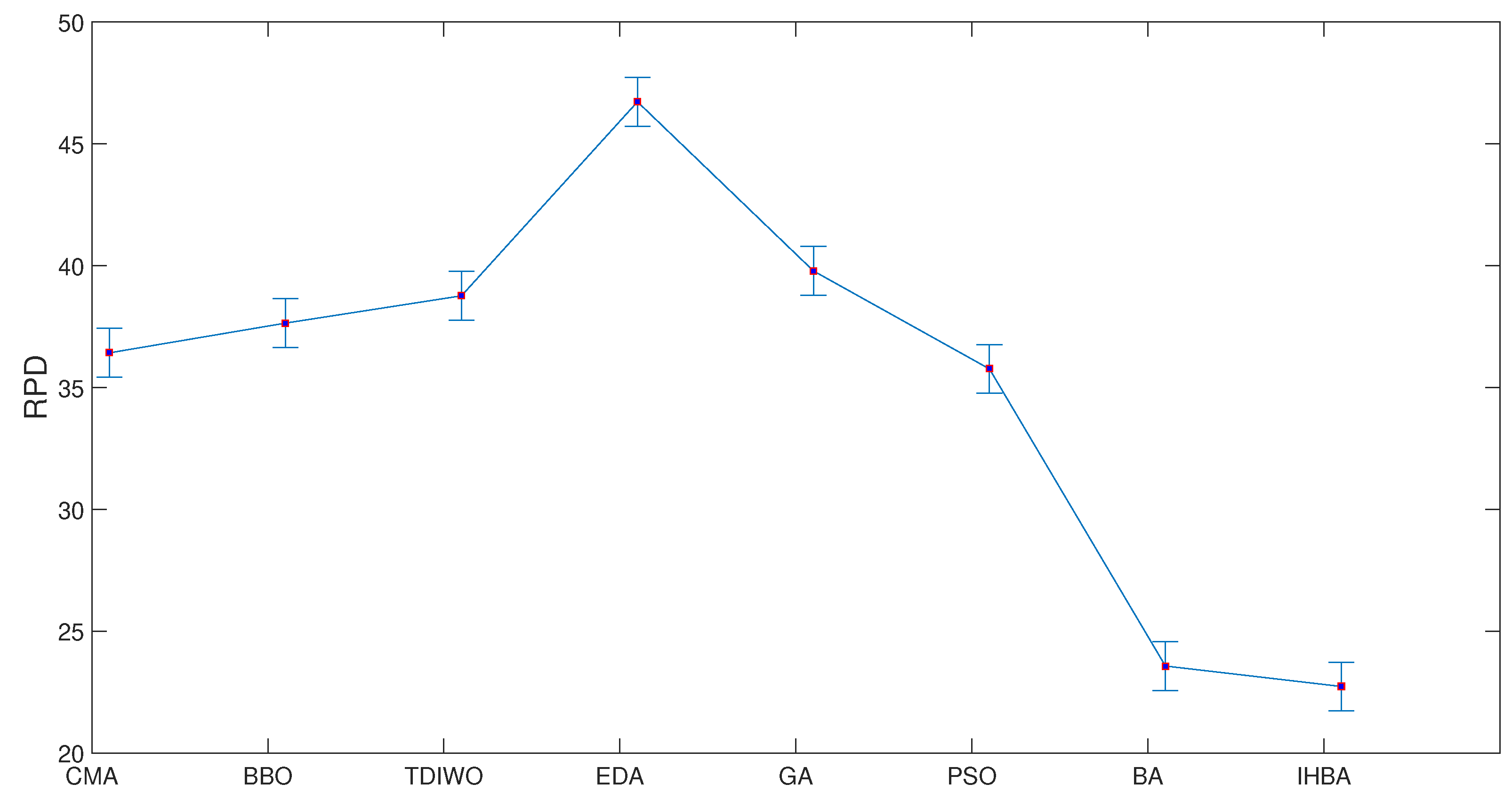
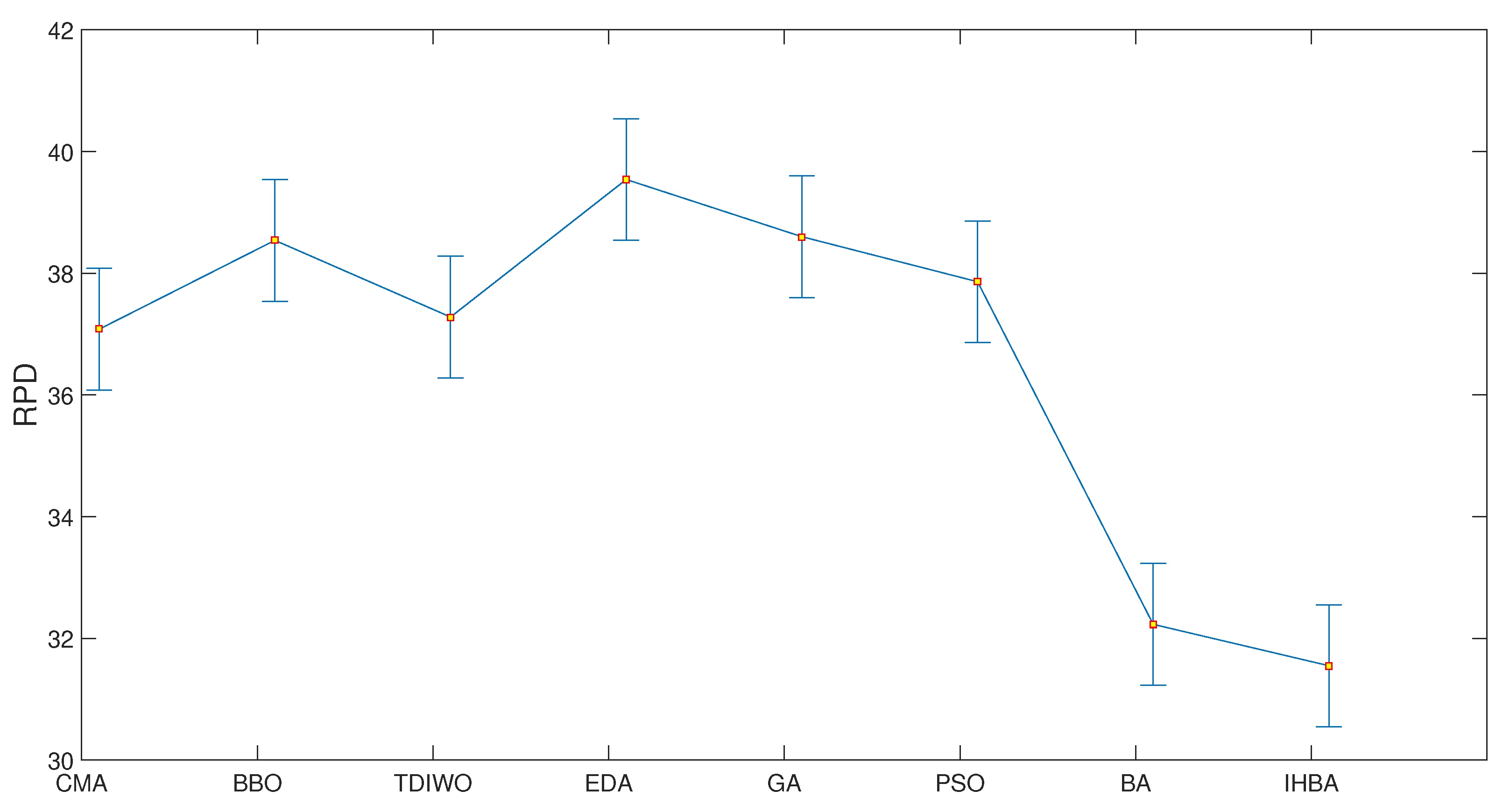
In this paper, an improved hybrid bat algorithm, IHBA, is proposed for solving the DAPFSP with maximum makespan based on the original bat algorithm. The main contributions of this paper are:

• The algorithm firstly designs the population classification to increase the diversity of the population and solve the difficult trade-off between convergence and diversity of the bat algorithm.
• A selection mechanism is used to update the speed and location of bats, solving the difficulty of the algorithm to trade-off exploration and mining capacity.
• Gaussian learning strategy and elite learning strategy assist the whole population to jump out of the local optimal frontier.

This paper is organized as described below. Section 2 reviews the closely related literature. Section 3 presents the DAPFSP problem and its mathematical model. In Section 4, the hybrid bat algorithm proposed in this paper is described in detail. In addition, the parameter calibration and simulation calculation results are analyzed in Section 5. In the last section, the paper is summarized, and future work is provided.

2. Literature Review

It is well known that the distributed permutation flowshop scheduling problem (PFSP) is one of the most well-known production scheduling problems. It has a strong engineering background by having the same work order on all machines. The problem has been shown to be a strong NP-hard problem when more than two machines are involved.The problem of distributed assembly permutation flowshop scheduling problem (DAPFSP) has been gaining attention and popularity among scholars and researchers. The most leading exponent is Hatami et al. [5], whose work is very enlightening. He was the first to optimize and improve the DAPFSP for modeling and studying complex supply chains in 2013. They also introduced the mixed integer linear programming model, proposed three construction algorithms, tested the variable neighborhood descent (VND) algorithm, and demonstrated the good performance of the VND algorithm in solving this scheduling problem. Similarly, he went on to expand on his previous paper by adding time for sequence-related setups in both the production and assembly stages [6]. In 2015, Hatami et al. [7] considered a distributed assembly scheduling problem with sequence-dependent setup times and the goal of minimizing production time. The setup times of both phases are sequence-dependent, which also lays the theoretical foundation for the sequences in this paper. Heuristics and meta-heuristics are also proposed to solve it. Based on his literature and views, many of these ideas and opinions have been studied and explored in greater depth by many scholars. Based on these rather cutting-edge ideas, many scholars have built on and deepened their research, and Ying et al. [8] extended the DAPFSP for flexible assembly and sequence-independent setup times in supply chains. Using completion time as an optimization criterion, construction heuristic and custom meta-heuristic algorithms are proposed to solve this emerging scheduling extension. Gonzalez-Neira et al. [9] studied a stochastic version of the DAPFSP and proposed a hybrid algorithm to solve the stochastic problem, integrating biased randomization and simulation techniques. Wang [10] introduced a just-in-time constraint between the two phases of the traditional DAPFSP to form a just-in-time DAPFSP to minimize the maximum weighted tardiness cost. A variable neighborhood search based on memory algorithm is proposed. From the above reviewed studies, it can be concluded that these scholars and researchers have extended and improved this problem, and most of them have an objective function based on minimizing the makespan, which provides a theoretical basis for the objective function in this paper.

Most scheduling problems are NP-hard and exact methods simply cannot find the optimal solution in reasonable computational time. Therefore, heuristic and meta-heuristic algorithms have been used to find the optimal solution and near-optimal solutions in reasonable computation time. Zhang et al. [11] pointed out that the DAPFSP is a typical NP-hard combinatorial optimization problem, and proposed an innovative three-dimensional matrix cube-based distribution estimation algorithm to address the difficulties of the proposed DAPFSP-T model. Likewise, Zhang et al. [12] also assumed this idea, and their team integrated the problem with two machine environments, distributed production and flexible assembly, which can assemble job processing into customized products, and proposed a mixed integer linear programming model to characterize the problem nature and solve the small-scale problem. An efficient modulo algorithm is further proposed. They affirm that the modal algorithm is an efficient algorithm to solve the DAPFSP, while some scholars prefer to use the greedy algorithm to solve the problem. For example, Pan et al. [13] solved a novel DAPFSP by proposing a mixed integer linear model, three construction heuristics, two variable neighborhood search methods, and an iterative greedy algorithm to obtain important problem-specific knowledge to improve the effectiveness of the algorithm. Similarly, Ochi et al. [14] studied the DAPFSP with the objective of minimizing completion time and, proposed an iterative greedy based approach called bounded search iterative greedy algorithm. Similarly, in order to coordinate production and transportation scheduling, Yang [15] proposed a novel DAPFSP-FABD model. The objective is to minimize the total cost of delivery and delay, and four heuristic algorithms, a variable neighborhood descent algorithm, and two iterative greedy algorithms are proposed. Liu et al. [16] proposed a memory algorithm for DAPFSP based on variable neighborhood search with the objective function of, i.e., makespan. And, the initialization based on NEH heuristic is applied to the product ordering. The neighborhood structure is introduced into VNS and used to perturb the job assignment of the factory and adjust the job order of the factory. Huang et al. [17] considered the DAPFSP with a total flow time criterion, and proposed an improved iterative greedy algorithm based on groupthink to solve the problem. It can be seen that the exact algorithm is no longer able to solve the problem, and this has promoted the development of heuristic and meta-heuristic algorithms, which can very definitely find the optimal solution as a solution to this scheduling problem.

More and more scholars are focusing more on the improvement of algorithmic aspects. For the no-wait flow shop scheduling problem that depends on time series, Hu et al. [18] proposed an enhanced differential evolutionary algorithm. Subsequently, Seidgar [19] took minimizing the weighted sum of expected completion time and average completion time as the solution objective and proposed four metaheuristic algorithms; namely, genetic algorithm, imperialistic competition algorithm, cloud theory-based simulated annealing, and adaptive differential evolution algorithm. Moreover, Li et al. [20] argued that the imperialist competition algorithm can solve the fuzzy distributed assembly flow shop scheduling problem. Furthermore, Al-Behadili et al. [21] proposed a multi-objective optimization model and particle swarm optimization solution method for the robust dynamic scheduling of permutation flow shops with uncertainty. Likewise, Zhang [22] emphasized that DAPFSP is a new generalization of the distributed displacement flow shop scheduling problem and the assembly flow shop scheduling problem, proposed an enhanced population-based metaheuristic genetic algorithm, and designed an effective crossover strategy based on local search to accelerate convergence. Li et al. [23] studied the minimization problem of DAPFSP and proposed a genetic algorithm with an enhanced crossover strategy and three different local searches. It is no coincidence that Mao et al. [24] advocated an improved discrete artificial bee colony algorithm to solve the DAPFSP with preventive maintenance operator, optimized by the completion time criterion. Moreover, a local search method with insertion and exchange operators is used to generate adjacent solutions in the hiring bee phase and the bystander bee phase. Song and Lin [25] jointly proposed a genetic programming hyperheuristic algorithm to solve the DAPFSP with sequence-dependent setup times, minimizing the completion time as the objective. For the improvement of the algorithm, these scholars further study the genetic algorithm and particle swarm algorithm. This also provides a reference basis for our subsequent simulation experiments.

3. Problem Description

The traditional distributed assembly permutation flowshop scheduling problem (DAPFSP) can be divided into two phases; namely, the production phase and the assembly phase. In this section, the two-stage DAPFSP problem is extended to a three-stage DAPFSP, named the production stage, the transportation stage, and the assembly stage, and the problem is described as follows.

The job $j\in \{1,2,\dots ,n\}$ consists of operations $O_{ij}$, $O_{Tj}$ and $O_{Aj}$. In the production stage, there are n work processes and f identical plants, and job $j\in \{1,2,\dots ,n\}$ needs to be assigned to any plant $l\in \{1,2,\dots ,f\}$ for processing, and each plant is equipped with the same m machines, $M=\left\{M_1,M_2,\dots ,M_m\right\}$, which correspond to the same assembly line shop for part processing. Operations $O_{ij}\in \{O_{1j},O_{2j},\dots ,O_{mj}\}$ are processed on machine $M_i$, $i=1,\dots ,m$ and require $p_{ij}$ time units. Machine $M_{ij}$ can process at most one job at a time. The production and transport operations $O_{Tj}$ will be executed on machine $M_T$ and take $p_{Tj}$ time units. The rule is that in each assembly permutation flowshop, all jobs need to be processed on the same path in the order of machine i, which is equivalent to first on machine $M_1$, then on $M_2$. This goes on, until the end on machine $M_m$. Parts belonging to the same product must be processed continuously, and no partial parts are allowed to pass through. All jobs start timing at time $t=0$ and on machine $i=1$.

The subsequent phase is the transport stage, which means that after the completion of the first one in the first stage of the product operation, the transport machine collects all parts of the product and moves to the assembly stage.

In the assembly stage, there are s products and an assembly machine $M_A$. Each product $r\in \{1,2,\dots ,s\}$ has a defined part of the operation. The assembly operation $O_{Aj}$ will be executed on the machine $M_A$ and uses $p_{Aj}$ time units. The rule is that the assembly of a product can only start when the work contained in the product is completed and the assembly machine is idle. Continuous processing stages are part of the same product operation. The next product operation can only be performed after all jobs belonging to a product have been processed.

From this, it is clear that the objective function of the problem is to determine the allocation of products to plants, and the sequence of parts and products to each plant in order to minimize the completion time or maximum completion time for all products. Based on the above description of the problem, the minimization of the completion time is denoted as $F_m\left|nwt\right|C_{max}$. To satisfy the above constraint, a feasible schedule $\pi =\left\{{\pi }_1,{\pi }_2,\dots ,{\pi }_n\right\}$ is found for n jobs, such that the completion time $C_{max}\left(\pi \right)$ is minimized. This is the same where $C_{max}\left(\pi \right)$ is also equivalent to the time to complete the last job on the last machine. The Equation (1) is as follows.

$$C_{max}\left(\pi \right)=\sum _{k=2}^n{D}_{{\pi }_{k-1},{\pi }_k}+\sum _{j=1}^m{P}_{{\pi }_n,j}$$

(1)

In the transportation phase, it is necessary to ensure that the completion time distance between two adjacent jobs is determined by the processing time of the two processes, independent of the other jobs in the arrangement. Therefore, the completion time distance is defined between each pair of jobs. The completion time distance between two adjacent job processes ${\pi }_{k-1}$ and ${\pi }_k$ is calculated as

$$C_{{\pi }_{k-1},{\pi }_k}=\underset{1\le i\le m}{max}\left\{\sum _{j=1}^i{P}_{{\pi }_{k-1},j}-\sum _{j=2}^i{P}_{{\pi }_k,j-1}\right\},k=2,3,\dots ,n$$

(2)

In order to build a mathematical model based on the above description, the constraints, parameters and variables are as follows.

Subject to,

$$\sum _{j=0,j\ne k}^n{X}_{j,k}=1,k\in \{1,2,\cdots ,n\}$$

(3)

$$\sum _{k=0,k\ne j}^n{X}_{j,k}=1,j\in \{1,2,\cdots ,n\}$$

(4)

$$\sum _{k=1}^n{X}_{0,k}=f$$

(5)

$$\sum _{j=1}^n{X}_{j,0}=f$$

(6)

$$X_{j,k}+X_{k,j}⩽1,k\in \{1,2,\cdots ,n-1\},k>j$$

(7)

$$\sum _{j=0}^{z_{r-1}}\sum _{k=z_{r-1}+1}^{z_r}{X}_{j,k}+\sum _{j=z_r+1}^{z_r}\sum _{k=z_{r-1}+1}^{z_r}{X}_{j,k}=1$$

(8)

$$r\in \{1,2,\cdots ,s\},z_r=\sum _{t=0}^r{n}_t$$

(9)

$$C_{i,j}⩾{\mathrm{C}}_{i-1,j}+p_{i,j},i\in \{1,2,\cdots ,m\},j\in \{1,2,\cdots ,n\}$$

(10)

$$\begin{array}{c}{C}_{i,j}⩾{\mathrm{C}}_{i-1,j}+p_{i,j}+\left(X_{j,k}-1\right)g\hfill \\ i\in \{1,2,\cdots ,m\},j\in \{1,2,\cdots ,n\},k\in \{0,1,2,\cdots ,n\},j\ne k\hfill \end{array}$$

(11)

$$\sum _{t=1,t\ne r}^s{Y}_{r,t}=1,r\in \{1,2,\cdots ,s\}$$

(12)

$$Y_{r,t}+Y_{t,r}⩽1,r\in \{1,2,\cdots ,s-1\},t>r$$

(13)

$$\begin{array}{c}{C}_r⩾C_{m,j}+p_r\hfill \\ j\in \left\{z_{r-1}+1,\cdots ,z_r\right\},r\in \{1,2,\cdots ,s\}\hfill \end{array}$$

(14)

$$\begin{array}{c}{C}_r⩾C_t+p_r+\left(Y_{r,t}-1\right)g\hfill \\ r\in \{1,\cdots ,s\},t\in \{0,\cdots ,s\},r\ne t\hfill \end{array}$$

(15)

$$TF⩾\sum _{r=1}^s{C}_r$$

(16)

$$X_{j,k}\in \{0,1\},j\in \{0,\cdots ,n\},k\in \{0,\cdots ,n\},j\ne k$$

(17)

$$Y_{r,t}\in \{0,1\},r\in \{0,\cdots ,s\},t\in \{0,\cdots ,s\},r\ne t$$

(18)

$$C_{i,j}⩾0,i\in \{1,2,\cdots ,m\},j\in \{1,2,\cdots ,n\}$$

(19)

$$C_r⩾0,r\in \{1,2,\cdots ,s\}$$

(20)

where $X_{jk}$ represents a binary variable. It is equal to 1 if job j is the predecessor of job k. Otherwise, $X_{jk}$ = 0. The same is true for $Y_{rt}$. The product r is equal to 1 if it is the predecessor of the product t. Otherwise, $Y_{rt}=0$. $C_{ij}$ is the completion time of job j on machine i, and $C_r$ is the completion time of product r. $p_r$ is the assembly time of product r, and $z_r$ is the total number of jobs contained in the first r products in the product sequence. In addition, g is a large enough positive number. $r_t$ is the number of jobs contained in product t. It is worth noting that $C_{0,j}=C_{i,0}=C_0=0$.

Equation (1) shows that the goal of the mathematical model is to minimize the completion time. The constraint sets (3) and (4) indicate that each job must have only one preceding job and one following job. Constraint sets (5) and (6) show that the preceding and following jobs of virtual job 0 are forced to be executed f times. Constraint set (7) ensures that a job cannot be both a predecessor and a successor of another job. Constraint set (8) ensures that jobs belonging to the same product are processed consecutively. Constraint set (9) indicates that job j can be processed on machine $i-1$ only after it is processed on machine i. Constraint set (10) indicates that job j can only be processed on machine i after completing the processing of job k if job j is a successor to job k, where g is positive and has a sufficiently large scale volume. The constraint sets (11) and (12) ensure that each product must have only one preorder and one subsequent job. Constraint set (13) ensures that a product cannot be both a preorder and a successor of another product. Constraint set (14) ensures that each product cannot enter the assembly stage before the production of the part of the job it contains is complete. Constraint set (15) shows that if product t is a preceding job of product r, then product r cannot start the assembly job until product t is completed. Constraint set (16) defines the minimum completion time. Constraint sets (17) to (20) define the domains of the decision variables.

The model uses a sequence-based variable and a set of $(min\{f,s\}+1)$ virtual parts. The sequence starts with a virtual part and ends with a virtual part. These virtual parts divide all parts into $min\{f,s\}$ subsequences, each corresponding to a plant. Parts belonging to the same product are never separated. Thus, the product sequence is implicitly included in the part sequence. For example, $s=4,n=8,m=2,f=2$.

Table 1. Machining time for parts and products.

Part	1	2	3		4	5	6	7	8
$M_1$	2		5	7		9	9	3	8	4
$M_2$	3		8	5		7	3	4	1	3
Product		1			2		3		4
$M_A$		9			8		7		6

shows the machining times of parts and products.

One of the feasible solutions is $x_{04}=x_{43}=x_{35}=x_{50}=x_{01}=x_{12}=x_{28}=x_{86}=x_{67}=x_{70}=1$. The sequence of parts is $\{0,4,3,5,0,1,2,8,6,7,0\}$, consisting of the subsequences $\{4,3,5\}$ and $\{1,2,8,6,7\}$.

4. Materials and Methods

To improve the local search capability of the algorithm, this section introduces the mathematical representation of feasible solutions, classification of populations, selection mechanism, domain structure and Gaussian learning strategy and elite learning strategy. A hybrid bat algorithm adapted to the three-stage DAPFSP problem is proposed.

4.1. Mathematical Expression of the Feasible Solution of the Three-Stage DAPFSP

The representation of feasible solutions is a crucial and important step in every meta-heuristic approach. The addition of a transportation process to the DAPFSP solved in this paper. The result is that the original expression for the process permutation of the PFSP is not adequate for this scheduling problem. Therefore, in this section, the feasible solution is divided into a sequence of products and a sequence of s processes based on the model of the three-stage DAPFSP model and the properties of the bat algorithm. Each sequence of these s processes corresponds to a product. The processes of a part can be viewed as the sequence of product assembly on the assembly flowshop.

In the production and transportation stages, parts need to be allocated one by one according to the product order. When allocating parts, their processes are sequentially arranged to the corresponding factories according to the process order of the product, and a minimum manufacturing cycle is obtained. Only after all the processes included in the current part are completed can the next part be produced. When a product has completed all processes, the product can proceed to the assembly stage for the installation and assembly stages. As an example, suppose a set of sequences f is used to represent a feasible solution, and each plant has one and only one solution. Each sequence is an ordering of all the parts assigned to that plant, indicating the order in which the parts enter the flow shop. Thus, the order of processed products in the assembly stage is also implied, and the feasible solution can be expressed as $\pi =\left\{{\pi }_1,{\pi }_2,\dots ,{\pi }_f\right\}$, where ${\pi }_k=\left({\pi }_{k,1},{\pi }_{k,2},\dots ,{\pi }_{k,\eta k}\right),k=1,2,\dots ,f$ is the sequence associated with sequence associated with plant k and ${\eta }_k$ is the total number of parts assigned to plant k. For the example in Section 3, the representation corresponding to this feasible solution is $\pi =\left\{{\pi }_1,{\pi }_2\right\}$ and ${\pi }_1=\{4,3,5\},{\pi }_2=\{1,2,8,6,7\}$.

In the feasible solution of the original DAPFSP problem, the first stage represents the arrangement of all N processes, and the second stage represents the plants to which these N processes are assigned respectively. In this section, the concept of product priority is introduced to determine the order of product assembly, and a novel feasible solution of the three-stage DAPFSP is proposed. Specifically, the feasible solution in the first stage is expressed as the processing priority of the product, and the parts assembly of each product is equal to the number of processes that constitute that product. The specific steps are, firstly, calculating the total processing time of the product at each stage and randomly initializing the sequence of products. Second, the first two products in the initial product sequence are selected for evaluation, and whichever sequence is better is chosen as the current sequence. Again, this is done by placing it among the product sequences that are already scheduled properly. Finally, an optimal schedule can be obtained to select the current best sequence for the next iteration of the process. The second stage is represented as the processing priority of all processes, where the processes belonging to the same product are arranged in a random order. The smaller the number of its columns, the higher the priority of the element values; the third stage is the plant priority assignment vector, where each part is represented as the plant assigned to the corresponding process. The specific steps are to assign a part of the processes to the factories one by one in order, then select a process and find the minimum completion time by placing it after the last process in each factory. The best part assignment is selected for the next iteration.

Table 2. Coding scheme.

Product Priority	2	1	2	3	3	2	1	3	3
Job	6	5	4	2	8	3	7	9	1
Factory Tasks	3	1	1	2	1	3	2	2	3

describes how the three-stage DAPFSP representation is decoded into a schedule. Suppose there are 3 products ($s=3$) consisting of 9 jobs ($n=9$) processed in 3 plants ($f=3$). The mathematical representation is $P_1=\{3,4,6\}$, $P_2=\{1,2,8,9\}$, $P_3=\{5,7\}$. According to the last two stages, called job sequence and factory assignment, it can be observed that jobs 5, 4, and 8 are assigned to the first factory and are processed in the order of 5, 4, and 8 according to the priority specified in layer 2. Then, it is instantly obtained that the partial scheduling of the factories can be decoded as ${\pi }_1=\{5,4,8\}$. Similarly, the partial scheduling of the remaining two plants can be decoded as ${\pi }_2=\{2,7,9\}$ and ${\pi }_3=\{6,3,1\}$, respectively. According to the values of the first stage specifying the product assembly priority, the value of 1 in the table corresponds to jobs 5 and 7 belonging to product 3. It can be concluded that after the processing stage, product 3 should be assembled first. In a similar way, it can be concluded that product 1 is assembled for the second time immediately after product 2.

In the context of the traditional representation of feasible solutions, the order of assembly of all products follows a first-come, first-served rule. This results in products being ranked in the processing stage in ascending order of the total completion time of their component operations. In contrast, the priority of products in the assembly phase is determined by the order of arrival at the assembly, and there is no way to specify it. This observation is confirmed by a study of the two-stage assembly scheduling problem by Tozkapan [26]. The efficiency may be higher if the sequence of operations in the processing phase is different from the sequence of operations in the assembly phase under the total delay objective. With a very late delivery date, for example, the assembly of the product may be delayed, even if the entire processing phase of the product’s component operations has been completed.

4.2. Population Classification

The optimization process is divided into two stages. The first stage is that when the individual bat is in a better search position and is close to the optimal solution, its loudness and pulse emission rate reach the best state. This process is called the search phase, its population is called the search-type population. The second stage is the population of bats in a disadvantaged search position; that is, the capture population, so two populations with different functions are obtained. After each iteration, by updating the search direction and step length, the loudness and pulse emission rate of the bat algorithm are improved to find the optimal solution. By adjusting the weights and deviations of the network, the difference between the average value and the standard deviation of the bat algorithm can be minimized.

4.2.1. Search-Type Population

The combination of the back propagation (BP) algorithm based on mean square error (MSE) and gradient descent method minimizes the mean square error [27]. The formula based on the mean square error measurement is shown in (21):

$$MSE(d,y)=\frac{1}{N}\sum _{n=1}^N{(d\left(n\right)-y\left(n\right))}^2$$

(21)

where $d\left(n\right)$ represents the n-th element of the required signal, and $y\left(n\right)$ represents the nth actual output. In the training process, the weight vector in the $(t+1)$ iteration is updated by (23). Where $\alpha$ is the learning rate or step length, ${\mathcal{W}}_t$ is the weight vector of the previous iteration and $g_t$ is the gradient vector, which can be calculated by (22) and (23).

$$w_{t+1}=w_t-\alpha g_t$$

(22)

$$g_t={\left.\frac{\partial e}{\partial w}\right|}_{w=w_t}=\left[\frac{\partial e}{\partial w_{11}}\cdots \frac{\partial e}{\partial w_{ij}}\dots \frac{\partial e}{\partial w_{nn}}\right]$$

(23)

In (23), e is the MSE error output in the t-th step of the training process and $\partial \mathrm{e}/\partial \mathrm{w}$ is derived from the MSE error on each element of the w vector. The weight is expressed as $w_{t+1}=w_t-{\alpha }_t{g}_t$, ${\alpha }_t$ will be adjusted to an appropriate value to achieve better convergence. At this time, suppose the probability pops of the search-type population, its loudness and pulse emission rate are updated to:

$$A_i^{t+1}={\alpha }_t\times A_i^t$$

(24)

$$r_i^{t+1}=r_i^o\left(1-e^{-wt}\right)$$

(25)

4.2.2. Captive Population

As a branch of the gradient descent method, the conjugate gradient method (CG) is applied to nonlinear unconstrained optimization problems. This method has strong local and global convergence [26,27,28]. According to the cloud computing resource scheduling problem, the CG method uses (26) to generate a weight sequence:

$$w_{t+1}^{\prime }=w_t^{\prime }+{\alpha }_t^{\prime }d$$

(26)

where ${\alpha }_t^{\prime }$ is the result of the line search method, which can be an exact line search or an inaccurate line search, which is expressed as a step size here. In (26), $d_t$ is in the descending direction, which is expressed as the search direction here, and its formula is shown in (27):

$$d_{t+1}=-g_{t+1}+{\beta }_t{d}_t$$

(27)

In (27), ${\beta }_t$ is the conjugate parameter, $g_{t+1}$ is the gradient of the objective function concerning the weight at step $t+1$, and represents the direction of the last step, and the first step is $d_0=-g_0$.

In the iterative process, the loudness $A_i$ and the pulse emission rate $r_i$ will also change. As the bat moves closer to its prey, its loudness will decrease, and the pulse emission rate will increase. At this time, the probability of the catching population is $po{p}_h$ and $po{p}_s+po{p}_h=1$. In summary, the loudness and pulse emission rate of the bat algorithm are updated to:

$$A_i^{t+1}={\alpha }_t^{\prime }\times A_i^t$$

(28)

$$r_i^{t+1}=r_i^o\left(1-e^{-w^{\prime }t}\right)$$

(29)

4.3. Selection Mechanism

When it comes to the bat algorithm as a learning algorithm, each individual in the population needs to learn from the individually optimal and globally optimal individuals in order to find the optimal solution. In the field of multi-objective optimization, there is no single optimal solution, and the optimal selection mechanism needs to be redesigned. Which strategy is used to update the individual optimal $p_{best}$ and the global optimal $g_{best}$ respectively, thus connecting the decision variable space and the objective space, is particularly important for weighing the exploration and exploitation capabilities of the algorithm evolution process. In this paper, we consider fully mining individuals with better diversity and convergence to assist populations to jump out of the local Pareto frontier. Three guides are selected from the searching and capturing populations to guide the entire individual bat flight, and how the guides are selected from the two populations is specified below.

Unlike the traditional bat algorithm, this algorithm first generates a set of $\theta$ with $\omega$ solutions and performs a local search process for the optimal solution in the set $\theta$. Subsequently, IHBA enters the iterative phase. In the iteration, the solution $\phi$ is selected using the selection mechanism in the set $\theta$. The solution $\phi$ is applied to the search phase and two partial sequences can be obtained, one for the solution ${\phi }_{Search}$ with the products and processes removed, and the other for the remaining part of the solution ${\phi }_{Captive}$. The local search for the products is applied to ${\phi }_{Captive}$, and the suboptimal solution ${\phi }_{Captive}^{\prime }$ is generated. IHBA again reinserts the removed products and jobs into ${\phi }_{Captive}^{\prime }$. This process is called the capture phase, and a complete solution ${\phi }^{\prime }$ is regenerated. A local search is performed on ${\phi }^{\prime }$ to generate ${\phi }^{″}$. Finally, acceptance criteria are used to determine whether the new solution ${\phi }^{″}$ updates the set.

Therefore, in scheduling problems, the selection mechanism is to select a solution from the solution set $\theta$ at the beginning of each iteration, and the selected solution is noted as $\phi$, and proceeds to the subsequent stages such as search and capture. In this scheduling problem, the minimum completion time and the number of iterations are often used as selection factors. So, the proposed selection mechanism consists of two random options, both of which have a 50% probability of being selected. That is, two solutions are randomly selected in the set $\theta$ and the one with the lower minimum completion time is chosen as $\phi$. Alternatively, two solutions are randomly selected in $\theta$, and the one with the lower number of iterations is chosen.

The main focus of $p_{best}$, $g_{best}$ and osd wizard selection mechanisms is on the target space, implying how to fully exploit the candidate solutions with good convergence and diversity in the target space. These wizards serve as a bridge between the target space and the decision variable space, and the new wizard selection mechanism can weigh the ability of exploration and exploitation of the decision variable space in an integrated way.

4.4. Three Neighborhood Structures Based on Insert Operator

To solve the three-stage DAPFSP problem, this paper introduces three neighborhood structures based on the INSERT operator, which constitutes the three-stage bat algorithm (3SBA). The insert operator is considered by many scholars as a superior performance operator, which is described as follows.

• Product-based Neighborhood (PBN)
  Regarding the order of product assembly, a randomly selected product is inserted into another random position.
• Factory-based Neighborhood (FBN)
  A process is randomly selected from the representation of the solution and assigned to another randomly selected plant. For this plant, all possible positions where jobs can be inserted are considered and the part of the job sequence with the earliest completion time is selected. It is worth noting that the sequence of jobs assigned to other plants remains unchanged during this process.
• Job Sequence-based Neighborhood (JSBN)
  A plant is randomly selected and its sequence of jobs is extracted from the solution representation. Next, a job is randomly selected from this partial sequence, and another location is randomly inserted. Finally, the jobs in this partial sequence along with their product priorities and plants are placed in an orderly manner in the distribution solution representation, which is partially the location belonging to that plant.

4.5. Local Search Method Based on Variable Neighborhood Structure

Based on the above three neighborhoods named PBN, FBN and JSBN, this section proposes a local search method with variable neighborhood search. Equation $n\left(s\right)$ denotes that the neighborhood structure and other parameters are consistent with the original bat algorithm, implying that the maximum number of iterations for each neighborhood at the same frequency is noted as $T_{max}$ and the frequency f is initialized as $f_0$. In 3SBA, all three neighborhoods are iterated sequentially, avoiding premature convergence throughout the search process.

Variable neighborhood descent (VND) is the simplest variant of variable neighborhood search [29]. It has been shown to be effective in solving the flow shop [30] and distributed scheduling problems [31]. VND searches for different neighborhood structures from minimum to maximum. First, starting from the initial solution, VND searches the first neighborhood to find the local optimum. Then, while searching the second region, if a better local optimum solution is found, the algorithm returns to the first neighborhood. Otherwise, it continues searching the third neighborhood and so on. The algorithm does not end until a local optimum is found with respect to all neighborhoods. Therefore, to facilitate the differentiation of the VNDs in this paper, two versions were developed based on the characteristics and features of the bat algorithm. The first one uses three neighborhood structures, named VND3BA, and the second one uses two neighborhood structures, named VND2BA, respectively. A VND that best fits the bat algorithm and the scheduling problem is selected by calibration through simulation experiments.

4.5.1. VND3BA Local Search Method Based on Three Neighborhood Structures

The first method is applied to each product contained in the plant. After removing each part of the product in succession, it is tested at all possible locations within the product. If a better manufacturing span is found, the part sequence is updated. This method runs until all parts contained in the plant have been taken into account and no further improvements are found; then, it can be stopped and ended. It can be named as Local Search Inside Product() and Part Local Search Inside Factory(). The former mainly searches individual products, while the latter searches the whole factory by calling the former, each in its own way.

The second method is a local search of the products within the factory. The principle of this method is to remove the products one by one from the beginning to the end and try to find the best position for them, equivalent to the optimal solution of this problem. If, in the process, a better manufacturing span is found, the sequence of parts in the plant is updated. The process is repeated until no products are found that can be improved.

The third method focuses on finding the most suitable location for a product that crosses plants. First, all plants are checked and the plant with the maximum completion time p is found. Then, the first product is removed and is tested in all possible locations in the remaining plants. If the generated best completion time is lower than the original completion time $C_p$, this product is inserted into the current location. The principle is that the algorithm iterates by finding the plant with the maximum completion time again, until a local optimum is found.

4.5.2. VND2BA Local Search Method Based on Two Neighborhood Structures

Since VND3BA considers the neighborhood of parts and the neighborhood of products separately, some available feasible solutions may be missed. Therefore, in this section, two local search algorithms are proposed to consider these two neighborhoods in an integrated manner.

The first approach explores the interior of the plant by extracting the range of products and finding the best location of the products within the plant. This step is to extend the scope of the local search. This method also adaptively finds the best part order for the product when inserting it.

The second approach exploits the local search capability of the bat algorithm itself to explore the optimal solution across plants. Therefore, it can be viewed as a combination of two processes named ProductLocalSearchBetweenFactories() and LocalSearchInsideProduct().

4.6. Gaussian Learning Strategy and Elite Learning Strategy

Gaussian learning strategy (GLS) [32] and elite learning strategy (ELS) [33] can assist individuals of bats to jump out of the local frontier and improve the local search ability of the algorithm. If the feasible solution is not updated many times, the whole bat population is most likely to fall into local optimum, and then only the GLS reset strategy can be executed, which is given by

$$x_i^{t+1}\sim N\left(\frac{x_{gbest}-x_{gbest,i}}{2},\left|x_{gbest}-x_{gbest,i}\right|\right)$$

(30)

The collaborative learning mechanism of $p_{best}$ and $b_{best}$ ensures that the exploration and exploitation capability of the entire bat population is enhanced, allowing the algorithm to quickly jump out of the local frontier to approximate the true frontier.

Although the use of GLS can assist individual bats to jump out of the local frontier, this strategy alone still cannot meet the requirements of the bat algorithm for solving the DAPFSP. To further improve the performance of the bat algorithm, ELS is introduced to solve the scheduling problem with the following mathematical expressions.

$$E_i\left(j\right)\sim E_i\left(j\right)+\left(x_{ub}\left(j\right)-x_{lb}\left(j\right)\right)N(0,1)$$

(31)

where $x_{ub}\left(j\right)$ and $x_{lb}\left(j\right)$ represent the upper and lower bounds of the j-th dimensional decision variable, respectively, and $N(0,1)$ represents the random number with a mean value of 0 and a variance of 1.

5. Simulation Results

5.1. Test Questions and Parameter Settings

In this section, the proposed IHBA is compared with the competitive memetic algorithm (CMA) [34], biogeography-based optimization algorithm (BBO) [35], estimation of distribution algorithm ( EDA) [36], genetic algorithm [19,21], and particle swarm optimization algorithm [20], and only one of these algorithms was selected for comparison from the literature [37]. So far, the three DIWO algorithms have proved to be the state-of-the-art algorithms for the considered problem with the parameters shown in

Table 3. Algorithms and Parameters.

Comparison	Parameters	Range
TDIWO	Initial population size	10
	Maximum population size	50
	permutation-based shift operator	5
	Max value	20
	Min value	1
	Control parameters	0.9
CMA	Selection probability of a subclass	0.5
	Selection probability of populations	0.5
	Number of populations	50
	Local search operator	100
BBO	Number of populations	40
	Elite retention number	10
	Max emigration rate	[0,1]
	Max migration rate	[0,1]
	Max mutation rate	[0,1]
EDA	Population size	50
	Probability vector	0.3
	Iterative Probability Sampling Parameters	0.4
GA	Number of populations	{40,50,60}
	Max number of iterations	300
	Crossover rate	[0.7, 0.9]
	Mutation rate	[0, 0.2]
PSO	Number of populations	2n
	Decreasing coefficient	0.975
	Crossover rate	[0,1]
	Variation rate	[0,1]
	Uniform random number	[0,1]
	Inertia weights	[0.4,0.9]
BA	Frequency	[0,1]
	Loudness	[1,2]
	pulse emission rate	[−1,1]
IHBA	Frequency	[0,1]
	Loudness	[1,2]
	pulse emission rate	[0,1]
	Step size	[0,1]

. All simulation experiments were implemented on the MATLAB r2020a platform. All programs were executed on an AMD A8-7100 Radeon [email protected] GHz and 12.0 GB RAM in Windows 10 operating system.

To calibrate the proposed IHBA, a total of 810 instances were randomly generated according to the literature [5,34] written by Hatami et al. These instances can be found in http://soa.iti.es/problem-instances, accessed on 1 September 2021. These instances combine four factors, including the number of jobs (n), the number of machines (m), the number of products (s), and the number of plants (f). Each factor has three levels, $n\in \{100,200,500\},m\in \{5,10,20\},f\in \{4,6,8\}$ and $s\in \{30,40,50\}$. Thus, a total of $3^4=81$ factor combinations are studied. The processing time in the production stage is randomly generated in the range $[1,99]$ with uniform distribution. The operation time of the transportation stage is obtained in the range $[\mathrm{l},99\mathrm{l}]$ with uniform distribution. The assembly operation time for the assembly stage is obtained in the range between $nl$ and $99nl$ with uniform distribution.

5.2. The Results and Discussion

Relative percentage deviations are the absolute deviations of a given measurement as a percentage of the mean, and can only be used to measure the deviation of a single measurement from the mean. In order to compare the efficiency between algorithms, the calculation of relative percentage deviations (RPD) is considered to compare and analyze these metaheuristic algorithms. Its formula is shown in (32).

$$RPD=\frac{C_{max}\left(\pi \right)-C_{max}{\left(\pi \right)}_{best}}{C_{max}{\left(\pi \right)}_{best}}\times 100\%$$

(32)

where $C_{max}\left(\pi \right)$ is the total completion time of the current algorithm, and $C_{max}{\left(\pi \right)}_{best}$ is the minimum value of $C_{max}\left(\pi \right)$ among all algorithms to be compared.

In this paper, the termination condition of the iteration is set to a maximum CPU runtime equal to $C\times m\times n$ milliseconds, and the results are calculated for C = 20, 40, and 60. Then, the results obtained from the calculation are compared with other algorithms. The methods used are the analysis of variance (ANOVA), which is widely used in parametric statistical procedures, and the Friedman test and Wilcoxon paired signed test, which are commonly used in nonparametric statistical procedures. These methods have been widely used and promoted in the recent scheduling literature.

5.2.1. Comparative Analysis at C = 20

When C = 20, the values of RPD for various heuristic algorithms are shown in

Table 4. The Average RPD Values at C = 20. It can be seen from the bold figures that the value of PRD of the proposed algorithm IHBA in this paper is smaller than that of other algorithms in the vast majority of combinatorial solutions, including the recognized TDIWO algorithm and the original bat algorithm.

Parameters				Algorithms for Comparison
$\mathit{m}$	$\mathit{n}$	$\mathit{s}$	$\mathit{f}$	CMA	BBO	TDIWO	EDA	GA	PSO	BA	IHBA
5	100	30	4	11.85	14.07	25.59	28.36	12.28	10.24	53.91	18.83
5	100	40	4	41.58	49.38	46.39	48.22	29.16	49.85	46.87	25.63
5	100	50	4	26.73	31.74	38.40	41.56	47.26	43.52	22.52	23.37
5	200	30	4	48.36	57.43	40.74	47.44	35.20	56.69	35.68	27.15
5	200	40	4	8.87	10.53	7.14	11.10	6.15	10.70	10.16	17.69
5	200	50	4	47.76	56.71	55.76	59.54	53.07	37.67	43.21	34.59
5	500	30	4	30.86	36.64	33.26	41.60	33.05	25.58	19.19	18.86
5	500	40	4	25.67	30.49	36.49	34.20	37.50	11.28	37.71	8.10
5	500	50	4	35.44	42.09	43.98	55.36	21.82	45.52	58.99	19.78
5	100	30	6	30.36	36.05	33.53	42.51	34.00	23.69	20.28	18.46
5	100	40	6	16.92	18.22	20.91	26.45	11.15	22.00	18.97	15.03
5	100	50	6	14.64	17.38	27.64	29.01	16.31	17.51	51.16	13.77
5	200	30	6	42.98	51.04	46.84	46.54	46.33	35.33	28.28	11.31
5	200	40	6	12.65	13.15	19.69	13.68	14.52	14.22	14.55	12.54
5	200	50	6	23.56	27.98	26.25	35.09	17.27	27.49	25.69	11.40
5	500	30	6	46.72	55.48	60.63	60.97	57.59	31.18	58.46	24.63
5	500	40	6	51.32	60.94	56.66	55.71	49.76	47.74	41.95	35.20
5	500	50	6	40.78	48.42	41.75	42.01	44.55	32.92	16.54	13.40
5	100	30	8	20.84	24.75	25.22	21.40	38.58	21.02	16.60	14.46
5	100	40	8	11.02	13.09	15.01	19.47	21.27	19.67	28.64	14.66
5	100	50	8	22.67	26.92	33.08	34.28	24.49	18.57	45.03	14.19
5	200	30	8	31.21	37.06	30.75	46.38	38.70	50.60	33.70	28.68
5	200	40	8	53.90	54.00	49.87	62.06	49.33	43.08	32.29	25.95
5	200	50	8	35.10	41.69	43.78	45.73	35.73	40.96	55.08	28.74
5	500	30	8	11.47	13.62	19.68	24.89	20.14	21.65	19.63	15.58
5	500	40	8	27.18	32.28	24.95	24.47	26.94	24.71	23.42	22.44
5	500	50	8	30.93	36.73	31.26	37.29	21.58	47.19	33.29	15.87
10	100	30	4	29.22	34.70	25.77	36.59	26.01	39.50	18.83	13.88
10	100	40	4	44.89	53.31	39.65	44.46	32.99	52.31	21.54	19.12
10	100	50	4	47.60	56.52	44.56	47.68	28.89	21.54	17.43	15.14
$\mathit{m}$	$\mathit{n}$	$\mathit{s}$	$\mathit{f}$	CMA	BBO	TDIWO	EDA	GA	PSO	BA	IHBA
10	200	30	4	42.81	50.84	45.18	52.77	23.63	27.72	15.36	16.31
10	200	40	4	24.49	29.09	24.96	30.24	22.21	24.33	24.06	18.05
10	200	50	4	22.92	25.34	35.40	46.44	33.68	30.87	29.50	20.82
10	500	30	4	32.87	39.03	42.94	48.66	33.78	28.67	28.91	26.93
10	500	40	4	50.92	60.46	59.45	67.94	30.49	26.25	22.15	22.22
10	500	50	4	25.84	30.68	29.11	33.74	20.88	28.21	17.38	13.10
10	100	30	6	23.73	26.31	25.34	36.70	23.18	22.91	18.00	11.04
10	100	40	6	38.41	39.99	36.67	44.55	20.91	25.07	20.69	23.65
10	100	50	6	29.15	34.62	38.62	41.89	27.51	27.88	27.73	21.81
10	200	30	6	39.89	37.37	31.57	36.12	26.45	29.34	29.94	24.69
10	200	40	6	36.05	34.69	42.13	34.93	23.31	24.19	23.62	19.12
10	200	50	6	30.22	35.89	49.16	32.23	26.75	20.67	24.09	21.13
10	500	30	6	42.37	50.32	48.31	50.49	48.61	31.90	32.61	26.39
10	500	40	6	29.31	21.06	21.56	33.01	21.97	25.72	25.27	23.94
10	500	50	6	59.07	70.15	66.60	64.97	24.49	27.74	26.04	20.91
10	100	30	8	51.95	61.69	49.99	52.54	29.46	29.25	26.85	19.78
10	100	40	8	34.00	36.63	32.67	40.62	22.16	24.44	28.81	20.86
10	100	50	8	56.42	67.00	50.65	54.65	55.99	51.22	22.92	28.90
10	200	30	8	41.14	48.85	49.44	46.66	56.14	22.03	21.86	21.52
10	200	40	8	49.89	59.25	51.00	48.80	52.47	42.32	21.99	22.23
10	200	50	8	41.96	49.82	50.83	50.00	45.85	33.87	45.36	20.07
10	500	30	8	40.46	48.05	39.82	46.89	40.35	36.53	24.49	21.79
10	500	40	8	33.12	39.33	29.86	43.19	21.71	21.22	23.33	18.57
10	500	50	8	22.82	25.22	29.75	30.31	22.57	21.79	20.48	20.39
15	100	30	4	41.00	48.68	48.43	33.07	27.57	30.33	27.09	18.56
15	100	40	4	32.39	38.46	41.61	50.28	25.80	25.73	29.15	17.36
15	100	50	4	24.60	29.21	27.17	25.18	21.45	25.28	22.54	20.74
15	200	30	4	39.11	46.44	39.60	46.76	33.83	40.48	23.17	27.04
15	200	40	4	32.44	38.52	44.61	46.40	30.73	30.90	28.91	25.84
15	200	50	4	35.44	36.46	27.70	28.21	28.96	21.37	26.87	27.48
15	500	30	4	29.43	34.94	29.08	37.33	38.61	27.30	21.71	24.60
15	500	40	4	39.05	30.74	32.58	35.84	34.42	32.77	27.07	23.55
15	500	50	4	33.60	39.90	29.44	36.31	27.27	36.57	25.20	22.54
15	100	30	6	48.79	57.94	44.76	54.99	45.33	47.37	29.07	24.60
15	100	40	6	35.70	42.39	34.74	41.65	32.14	45.68	24.84	24.55
15	100	50	6	30.59	34.45	31.89	33.88	34.72	34.40	29.02	26.06
15	200	30	6	48.61	57.73	34.31	62.97	28.05	24.32	21.15	21.04
15	200	40	6	36.57	43.43	32.65	41.21	37.58	31.90	29.96	28.62
15	200	50	6	19.02	22.59	25.25	32.25	25.43	20.72	23.85	20.05
15	500	30	6	34.44	39.02	36.17	39.27	43.01	33.42	33.74	30.71
15	500	40	6	38.32	45.50	38.05	42.53	32.75	40.05	20.60	20.55
15	500	50	6	34.04	40.43	40.17	45.40	40.42	34.26	29.71	29.51
15	100	30	8	28.09	33.36	24.98	29.91	30.08	53.29	25.50	24.36
15	100	40	8	31.40	37.29	37.76	38.73	33.05	46.61	28.17	20.90
15	100	50	8	44.26	52.56	49.95	51.98	34.90	49.19	28.10	20.38
15	200	30	8	32.96	39.14	33.75	48.87	25.10	27.53	24.32	21.47
15	200	40	8	26.57	31.55	34.71	42.07	22.66	27.82	24.17	28.35
15	200	50	8	23.99	28.49	28.64	32.36	25.55	20.04	15.67	15.14
15	500	30	8	44.80	53.20	42.29	43.54	52.56	32.56	21.67	22.26
15	500	40	8	53.71	63.78	45.43	54.28	44.49	57.55	21.57	22.33
15	500	50	8	39.05	46.38	42.36	45.63	56.73	27.47	29.36	21.82
average				34.33	39.71	37.09	41.40	32.09	31.52	27.69	21.15

. It can be seen from the bold figures that the value of PRD of the proposed algorithm IHBA in this paper is smaller than that of other algorithms in the vast majority of combinatorial solutions, including the recognized TDIWO algorithm and the original bat algorithm. Only in these 5 sets of data (1) $m=5,n=100,s=30$ and $f=4$, (2) $m=5,n=200,s=40$ and $f=4$, (3) $m=10,n=100,s=50$ and $f=8$, (4) $m=15,n=200,s=50$ and $f=4$, (5) $m=15,n=200,s=40$ and $f=8$, IHBA is 5–10% smaller than the other algorithms. Meanwhile, IHBA not only obtains the lowest relative percentage deviation value, but also the smallest average RPD value, which is 21.15%, with an error of about 0.83% from the optimal value. This is good proof that the IHBA algorithm has a strong advantage and superiority. It can also be seen that the GA and PSO performance is also very good, with average RPD values of 32.09% and 31.52%. Although TDIWO is not satisfactory in this comparison, it is significantly better than BBO and EDA. The most surprising is the original bat algorithm, with a result of 27.69, which is second only to the algorithm proposed in this paper. This also shows that the bat algorithm itself has better performance and has stronger search capability.

Then, the results of the descriptive statistics of the Friedman test were calculated for the case of C = 20, as shown in

Table 5. The Descriptive Statistics Achieved by the Friedman Test at C = 20 and $\alpha$ = 0.05. The bold figures indicate the comparison between algorithms.

Algorithms	Rank	n	Mean	Std. Deviation	Min	Max
CMA	4.81	4050.00	1.17	0.92	0.00	7.05
BBO	4.92	4050.00	1.47	1.30	0.00	7.70
EDA	7.01	4050.00	16.89	12.80	0.00	50.37
TDIWO	3.36	4050.00	0.99	0.96	0.00	4.82
GA	3.99	4050.00	1.43	1.36	0.00	4.61
PSO	3.69	4050.00	1.31	1.25	0.00	5.35
BA	3.38	4050.00	1.00	0.95	0.00	4.47
IHBA	2.60	4050.00	0.74	0.71	0.00	5.51
p-value	0.00

, where N is the number of test cases and takes the value of 4050. The minimum value of each item derived in the algorithm is marked in bold. The p-value calculated for the test statistic is 0 when the significance level $\alpha$ = 0.05, which is less than or equal to 0.05. This indicates that there are significant differences between the algorithms used for comparison. The following conclusions can be clearly seen through Table 5. The rank of IHBA is only 2.60, which is close to one-half of CMA, BBO and TDIWO, while it is smaller than the ranks of GA, PSO and the original bat algorithm by 1.39, 1.09 and 0.78, respectively. Although IHBA does not take the best value in terms of maximum value, it means that standard deviation and minimum value are the smallest among all algorithms. The comparison between the groups also shows that the ranking of EDA is even more than three times that of IHBA, indicating the worst performance of the algorithm, which echoes the results and analysis in Table 4. In addition, it can also be seen by the mean and standard deviation that the three algorithms of DIWO are very close to the proposed algorithm.

Next, the non-parametric test for paired samples is the Wilcoxon paired signed test method used. This method was developed based on the signed test for paired observations, and is more effective than the traditional test with positive and negative signs alone. The observed data are generally considered to be significantly different when p is less than 5%. When p is greater than or equal to 5%, the difference in the data is considered insignificant. The results of the Wilcoxon paired signed test for this paper are given in

Table 6. The Wilcoxon paired signed test result at C = 20 and $\alpha$ = 0.05.

Algorithms for Comparison	R+	R−	Bonding Value	p-Value
IHBA VS CMA	756	3168	126	0.00
IHBA VS BBO	2341	274	1435	0.00
IHBA VS EDA	3840	100	110	0.00
IHBA VS TDIWO	1791	817	1442	0.00
IHBA VS GA	3113	783	154	0.00
IHBA VS PSO	2881	829	341	0.00
IHBA VS BA	2873	907	270	0.00

, assuming that there is no difference between each pair of algorithms ($\alpha$ = 0.05). $R+$ in the table represents positive differences and $R-$ represents negative differences. In the results for each pair of algorithms, the sum of $R+$, $R-$ and bonding values is equal to n in Table 5. It can also be seen in Table 6 that the p-values in the last column are equal to 0 and all are less than 0.001, indicating that the differences between the algorithms compared are statistically significant with respect to 0. In other words, there is a significant difference between IHBA and the other algorithms.

Finally, in order to make the observations more visual and relevant, this section analyzes and interprets the results of the ANOVA analysis for the eight algorithms. The methods used are the mean plot and the minimum difference method interval, and Figure 1 shows the plotted plots with 95% confidence level. It can be very clearly seen that the best performance is IHBA, which beats the other comparison algorithms by a more significant margin. The bat algorithm also has some advantages, while GA and PSO continue to perform consistently, and the EDA algorithm has the worst performance, followed by BBO.

5.2.2. Comparative Analysis at C = 40

The lower the RPD, the better the performance of the algorithms. When C takes the value of 40, the average RPD of these eight algorithms is shown in

Table 7. The Average RPD Values at C = 40. It can be seen from the bold figures that the value of PRD of the proposed algorithm IHBA in this paper is smaller than that of other algorithms in the vast majority of combinatorial solutions, including the recognized TDIWO algorithm and the original bat algorithm.

Parameters				Algorithms for Comparison
m	n	s	f	CMA	BBO	TDIWO	EDA	GA	PSO	BA	IHBA
5	100	30	4	17.00	21.80	22.45	25.09	18.96	17.93	18.42	17.76
5	100	40	4	45.33	46.15	47.52	54.11	49.00	44.16	30.39	29.30
5	100	50	4	31.97	35.80	36.86	49.68	42.45	40.10	26.74	25.79
5	200	30	4	48.36	46.67	48.06	56.50	52.94	47.03	29.99	28.92
5	200	40	4	8.76	9.22	9.50	10.91	10.09	9.03	7.37	7.49
5	200	50	4	52.88	55.13	56.77	70.34	57.50	52.03	35.04	33.79
5	500	30	4	33.25	35.74	36.80	45.17	37.22	33.69	21.18	20.42
5	500	40	4	30.58	32.43	33.39	43.34	32.52	29.70	20.40	19.68
5	500	50	4	40.10	45.33	46.68	51.02	45.22	41.34	30.30	29.22
5	100	30	6	32.98	35.93	36.99	45.65	37.06	33.62	21.29	20.53
5	100	40	6	18.50	21.02	21.64	23.98	21.42	19.55	14.14	13.63
5	100	50	6	19.69	23.73	24.43	28.23	22.68	21.36	19.19	18.50
5	200	30	6	26.49	26.29	27.66	39.61	29.83	24.77	26.50	25.55
5	200	40	6	15.01	14.91	15.35	19.08	16.28	14.90	11.01	10.62
5	200	50	6	25.67	28.63	29.48	33.31	29.19	26.55	17.68	17.05
5	500	30	6	53.74	56.76	58.44	73.33	57.88	52.64	36.23	34.94
5	500	40	6	55.75	55.55	57.20	69.71	59.65	53.63	35.43	34.17
5	500	50	6	43.22	42.37	43.62	55.23	46.38	41.51	23.60	22.76
5	100	30	8	23.37	22.88	23.55	34.36	28.11	25.93	16.95	16.34
5	100	40	8	12.91	15.25	15.70	21.51	18.43	17.53	14.66	14.13
5	100	50	8	27.28	30.22	31.12	37.12	29.63	27.20	20.94	20.20
5	200	30	8	32.68	36.60	37.69	47.78	43.46	40.30	28.25	27.24
5	200	40	8	52.07	53.18	54.76	67.27	57.82	51.16	32.42	31.26
5	200	50	8	39.79	42.05	43.30	52.17	45.00	41.17	30.87	29.76
5	500	30	8	13.78	18.65	19.20	24.48	20.64	19.80	15.01	14.47
5	500	40	8	27.86	26.19	26.96	33.95	29.73	26.41	18.14	17.49
5	500	50	8	32.65	33.74	34.75	39.64	37.96	34.47	23.02	22.20
10	100	30	4	29.60	31.11	32.03	38.46	35.52	32.19	19.82	19.12
10	100	40	4	45.50	44.04	45.35	53.25	49.56	44.10	25.93	25.01
10	100	50	4	49.07	47.68	49.10	55.52	45.70	39.44	21.63	20.86
10	200	30	4	45.82	47.69	49.11	53.88	44.99	39.63	22.34	21.54
10	200	40	4	25.92	27.02	27.82	33.28	28.76	25.91	17.76	17.13
10	200	50	4	27.61	34.35	35.37	44.02	36.05	34.01	24.29	23.42
10	500	30	4	37.90	41.87	43.11	51.38	41.84	38.23	25.91	24.99
10	500	40	4	56.38	60.21	62.00	68.23	54.72	48.43	28.21	27.20
10	500	50	4	28.26	29.98	30.87	35.75	31.20	28.24	17.58	16.95
10	100	30	6	24.88	28.32	29.16	34.85	29.29	26.62	16.93	16.33
10	100	40	6	37.98	38.85	40.00	44.41	38.07	33.11	21.18	20.42
10	100	50	6	33.79	36.90	38.00	44.58	36.98	33.77	22.89	22.08
10	200	30	6	35.92	33.67	34.67	41.10	37.17	31.85	21.99	21.20
10	200	40	6	37.25	35.82	36.88	42.21	36.17	31.53	20.65	19.92
10	200	50	6	38.04	37.59	38.71	45.01	36.10	32.61	21.49	20.72
10	500	30	6	46.53	47.79	49.21	61.79	50.37	45.47	29.42	28.37
10	500	40	6	23.74	24.24	24.96	30.50	28.26	24.42	18.70	18.03
10	500	50	6	64.63	64.65	66.57	70.69	57.97	50.29	28.49	27.47
10	100	30	8	54.00	52.63	54.20	60.53	50.90	44.14	25.66	24.75
10	100	40	8	34.09	35.23	36.28	41.28	35.28	30.99	20.93	20.19
10	100	50	8	57.45	55.22	56.86	71.34	62.21	55.35	32.63	31.47
10	200	30	8	46.02	46.46	47.84	62.84	48.94	44.18	26.87	25.91
10	200	40	8	52.85	50.98	52.49	66.10	56.25	50.27	29.48	28.43
10	200	50	8	47.07	48.29	49.72	61.41	50.43	45.62	30.37	29.28
10	500	30	8	42.35	43.19	44.48	54.72	46.69	41.91	25.91	24.98
m	n	s	f	CMA	BBO	TDIWO	EDA	GA	PSO	BA	IHBA
10	500	40	8	33.77	36.02	37.09	41.90	34.89	30.75	19.49	18.80
10	500	50	8	25.67	27.33	28.15	33.70	28.23	25.67	17.94	17.30
15	100	30	4	45.58	41.72	42.96	49.30	42.42	37.24	22.85	22.03
15	100	40	4	37.12	41.78	43.02	48.80	39.68	36.02	23.45	22.61
15	100	50	4	26.73	26.14	26.92	32.19	28.31	25.40	17.58	16.95
15	200	30	4	41.30	42.56	43.83	52.07	45.60	41.01	26.03	25.10
15	200	40	4	38.14	41.52	42.75	50.08	41.41	37.85	25.60	24.69
15	200	50	4	32.87	29.61	30.49	37.92	32.99	28.26	19.83	19.12
15	500	30	4	30.84	32.48	33.45	43.74	36.42	33.12	22.05	21.27
15	500	40	4	33.79	31.78	32.73	41.74	38.04	32.94	22.99	22.17
15	500	50	4	33.97	33.86	34.87	41.54	37.61	33.56	21.89	21.11
15	100	30	6	50.00	50.54	52.04	63.44	55.40	49.58	30.39	29.30
15	100	40	6	37.24	38.07	39.20	47.16	43.02	38.93	25.14	24.24
15	100	50	6	31.99	32.12	33.08	42.17	37.02	33.53	23.45	22.62
15	200	30	6	46.42	49.68	51.16	57.21	47.41	41.07	23.68	22.84
15	200	40	6	37.18	37.59	38.71	48.40	41.36	36.98	24.93	24.04
15	200	50	6	22.07	25.67	26.43	32.98	26.90	25.00	18.22	17.57
15	500	30	6	36.18	36.69	37.78	49.21	41.73	37.80	26.71	25.75
15	500	40	6	40.22	40.41	41.61	49.63	43.93	39.38	24.02	23.16
15	500	50	6	37.83	40.38	41.58	52.01	43.47	39.74	27.10	26.13
15	100	30	8	28.52	28.29	29.13	36.98	36.98	33.98	23.22	22.40
15	100	40	8	35.13	36.47	37.55	45.88	41.64	38.30	25.34	24.43
15	100	50	8	48.44	49.52	50.99	59.18	52.38	47.24	28.95	27.92
15	200	30	8	34.93	39.03	40.18	45.89	38.40	34.53	22.35	21.55
15	200	40	8	30.64	34.72	35.75	40.93	34.33	31.45	22.20	21.40
15	200	50	8	26.77	28.68	29.53	35.95	29.46	26.75	16.96	16.36
15	500	30	8	46.30	44.56	45.88	59.87	49.81	44.39	26.53	25.58
15	500	40	8	53.77	52.40	53.96	64.99	59.12	52.58	30.33	29.24
15	500	50	8	42.17	43.07	44.35	59.72	47.71	43.28	27.58	26.59
average				36.42	37.64	38.76	46.72	39.78	35.76	23.57	22.73

. As can be seen in the last row, the average value of IHBA is 22.73%, which is significantly lower than the average value of other algorithms including the original bat algorithm. It shows that the IHBA algorithm is more efficient than the other metaheuristic algorithms, while BA performs second, with an average RPD of 23.57%. Compared with Table 7, it can be concluded that the RPD value of IHBA changes from the original 21.15 to the current 22.73, as the value of C is taken to increase, which shows that the value of RPD of IHBA increases with the increase of the number of iterations and time. In addition, PSO with a mean value of 35.76% is significantly better than GA and the other four heuristics. Meanwhile, EDA has the largest value and its performance is the worst, which is also consistent with the results in Table 4.

Table 8. The Descriptive Statistics Achieved by the Friedman Test at C = 40 and $\alpha$ = 0.05. The bold figures indicate the comparison between algorithms.

Algorithms	Rank	n	Mean	Std. Deviation	Min	Max
CMA	4.81	4050.00	1.17	0.92	0.00	7.05
BBO	4.92	4050.00	1.47	1.30	0.00	7.70
EDA	7.01	4050.00	16.89	12.80	0.00	50.37
TDIWO	3.36	4050.00	0.99	0.96	0.00	4.82
GA	3.43	4050.00	0.93	0.87	0.00	4.44
PSO	4.22	4050.00	1.11	0.96	0.00	5.98
BA	3.06	4050.00	0.79	0.76	0.00	4.67
IHBA	2.94	4050.00	0.77	0.75	0.00	4.71
p-value	0.00

describes the results of the Friedman test calculations. As can be seen at a glance from the rankings, IHBA has a mean rank of 3.06, which is the smallest value among these algorithms. The next best performer is TDIWO, which also has a better performance, but its standard deviation is 0.89, which is larger than CMA, GA, and PSO. It can be seen from the mean and standard deviation that IHBA has values of 0.79 and 0.76, respectively, which are also the smallest values among all algorithms. The performance of EDA is still the worst, with its average rank, mean, standard deviation, and maximum value all being at a disadvantage. The performance of EDA is still the worst, with its ranking, mean, standard deviation and maximum value being at a disadvantage. In particular, the mean value is as high as 32 times that of IHBA. The p-value in the last row is 0, which is less than 0.05, indicating that the difference between the algorithms has statistical significance. This difference is not due to chance sampling, but rather, the difference between the two groups of algorithms is significant.

The results obtained from the Wilcoxon paired signed test are shown in

Table 9. The Wilcoxon paired signed test result at C = 40 and $\alpha$ = 0.05.

Algorithms for Comparison	R+	R−	Bonding Value	p-Value
IHBA VS CMA	671	3280	99	0.00
IHBA VS BBO	2434	220	1396	0.00
IHBA VS EDA	3879	100	71	0.00
IHBA VS TDIWO	1933	710	1407	0.00
IHBA VS GA	3198	804	48	0.00
IHBA VS PSO	2149	540	1361	0.00
IHBA VS BA	3050	948	52	0.00

. The p-values in the last column are all equal to 0, which is less than 0.05. It shows that the differences between these algorithms are statistically significant, and that there are significant differences between IHBA and the other algorithms. This also reconfirms the conclusion that C = 20. More definitely, it explains that IHBA is an effective group intelligence algorithm with outstanding performance.

Finally, in this section, EDA is excluded from the mean plot. The reason is that the algorithm is too intrusive and its performance is too poor. As can be seen in Figure 2, IHBA is once again stronger than the other metaheuristic algorithms by a margin. Once again, the variability between the algorithms is proven to be at a significant level. Since the LSD test has the highest sensitivity, Figure 2 verifies from the side that IHBA is an algorithm that performs well and can reach Pareto optimality.

5.2.3. Comparative Analysis at C = 60

Table 10. The Average RPD Values at C = 60. It can be seen from the bold figures that the value of PRD of the proposed algorithm IHBA in this paper is smaller than that of other algorithms in the vast majority of combinatorial solutions, including the recognized TDIWO algorithm and the original bat algorithm.

Parameters				Algorithms for Comparison
$\mathit{m}$	$\mathit{n}$	$\mathit{s}$	$\mathit{f}$	CMA	BBO	TDIWO	EDA	GA	PSO	BA	IHBA
5	100	30	4	21.03	21.53	21.14	22.70	22.35	19.26	20.68	20.84
5	100	40	4	45.06	46.69	45.56	47.61	45.75	46.63	40.83	40.08
5	100	50	4	37.12	37.79	37.41	41.04	39.73	40.82	34.18	33.43
5	200	30	4	47.20	49.43	47.57	50.02	47.74	49.63	42.30	41.33
5	200	40	4	11.03	12.18	11.01	13.06	11.75	9.04	9.69	9.66
5	200	50	4	53.25	54.80	53.76	55.71	55.59	55.49	47.22	46.29
5	500	30	4	34.70	36.10	34.82	37.18	36.60	35.23	29.30	28.58
5	500	40	4	31.75	32.82	32.21	33.83	34.12	31.45	26.98	26.47
5	500	50	4	42.52	43.67	42.61	44.96	43.45	43.58	39.09	38.53
5	100	30	6	34.71	36.05	34.81	37.16	36.76	35.19	29.28	28.57
5	100	40	6	20.98	21.90	20.95	23.25	21.89	20.05	18.20	17.91
5	100	50	6	23.38	23.98	23.58	25.45	24.73	22.48	22.43	22.41
5	200	30	6	31.96	35.07	37.00	39.41	38.96	40.95	34.61	35.04
5	200	40	6	16.42	17.30	16.77	18.65	17.45	15.14	13.98	13.78
5	200	50	6	27.68	28.91	27.69	30.09	28.80	27.43	23.77	23.27
5	500	30	6	54.30	55.62	54.94	56.61	57.10	56.33	48.11	47.22
5	500	40	6	54.49	56.34	55.21	57.09	56.11	57.05	48.51	47.50
5	500	50	6	41.94	43.79	42.47	44.65	43.88	43.44	34.55	33.48
5	100	30	8	25.59	26.71	26.03	28.52	27.71	26.63	22.52	22.01
5	100	40	8	17.68	18.42	17.70	20.40	19.22	17.77	17.30	17.20
5	100	50	8	29.38	30.33	29.67	31.41	30.96	28.81	26.43	26.14
5	200	30	8	38.13	39.23	37.99	41.76	39.92	41.60	36.36	35.72
5	200	40	8	52.43	53.78	52.29	54.87	54.22	54.77	45.26	44.12
5	200	50	8	41.91	43.09	42.34	44.51	43.33	43.64	39.47	38.96
5	500	30	8	19.50	20.11	19.62	22.39	21.30	19.79	18.05	17.81
5	500	40	8	27.99	29.62	28.36	30.23	29.02	27.91	24.85	24.40
5	500	50	8	34.15	35.61	34.35	37.10	34.76	35.59	30.98	30.35
10	100	30	4	31.67	33.18	31.67	34.69	32.85	33.03	27.60	26.88
10	100	40	4	43.96	46.09	44.36	46.88	44.68	46.02	37.74	36.66
10	100	50	4	43.84	46.31	44.35	45.13	44.90	42.43	33.92	32.84
10	200	30	4	42.87	44.87	43.17	44.57	44.00	41.96	33.59	32.56
10	200	40	4	27.34	28.72	27.49	29.64	28.52	27.10	23.92	23.48
10	200	50	4	33.34	33.74	33.22	36.41	35.74	35.00	30.23	29.70
10	500	30	4	39.57	40.71	39.83	41.94	41.52	40.24	34.40	33.72
10	500	40	4	52.70	54.68	53.09	54.06	54.32	51.76	41.54	40.34
10	500	50	4	29.19	30.54	29.38	31.66	30.37	29.12	24.41	23.79
10	100	30	6	27.57	28.64	27.42	30.04	29.20	27.50	23.03	22.46
10	100	40	6	36.71	38.24	36.72	38.26	37.51	35.65	30.23	29.51
10	100	50	6	35.13	36.28	35.43	37.48	36.72	35.36	30.41	29.81
10	200	30	6	35.05	36.48	25.00	36.74	35.55	34.76	30.63	30.04
10	200	40	6	34.94	36.12	35.38	36.55	35.66	33.93	28.12	28.19
10	200	50	6	35.39	36.64	36.45	37.23	36.67	34.44	29.26	28.63
10	500	30	6	46.59	48.16	47.09	49.07	48.84	48.23	40.39	39.48
10	500	40	6	26.68	27.32	26.11	28.68	27.47	26.53	24.27	23.91
10	500	50	6	56.43	59.00	57.28	57.13	57.08	54.35	43.68	42.38
10	100	30	8	48.53	51.05	49.11	49.84	49.34	47.57	38.91	37.82
10	100	40	8	34.03	35.49	34.05	35.77	34.99	33.26	28.97	28.39
10	100	50	8	55.22	57.60	55.79	58.18	56.95	58.49	47.45	46.11
10	200	30	8	45.36	46.91	46.02	47.81	48.24	46.78	37.80	36.78
10	200	40	8	50.53	52.60	51.26	53.33	52.42	52.97	42.70	41.47
10	200	50	8	46.91	48.40	47.51	49.32	48.93	48.44	41.12	40.28
10	500	30	8	42.52	44.27	42.80	45.17	44.25	44.08	36.49	35.56
10	500	40	8	33.76	35.52	33.71	35.51	34.98	32.76	27.86	27.22
$\mathit{m}$	$\mathit{n}$	$\mathit{s}$	$\mathit{f}$	CMA	BBO	TDIWO	EDA	GA	PSO	BA	IHBA
10	500	50	8	27.20	28.20	27.44	29.46	28.55	26.81	23.54	23.11
15	100	30	4	40.34	42.38	41.45	42.08	40.91	39.70	33.27	32.44
15	100	40	4	38.10	39.33	38.25	40.20	39.79	37.87	31.88	31.17
15	100	50	4	26.98	28.40	27.39	29.22	27.89	26.61	23.70	23.28
15	200	30	4	41.62	43.31	41.89	44.27	42.96	43.04	36.18	35.32
15	200	40	4	39.16	40.30	39.57	41.55	40.85	39.73	33.99	33.32
15	200	50	4	31.61	33.30	31.82	33.23	32.38	30.95	27.72	27.25
15	500	30	4	33.42	34.77	33.52	36.15	35.46	34.69	29.66	29.04
15	500	40	4	34.80	35.60	34.57	36.97	35.72	35.69	31.01	30.37
15	500	50	4	34.45	36.19	34.63	36.96	35.38	35.24	30.42	29.76
15	100	30	6	49.72	51.74	49.98	52.56	51.34	52.26	43.13	42.01
15	100	40	6	38.52	40.11	38.74	41.52	39.67	40.49	34.42	33.64
15	100	50	6	33.84	35.10	34.11	36.57	35.26	35.23	30.97	30.42
15	200	30	6	45.12	47.58	44.69	46.53	46.53	44.27	36.10	35.07
15	200	40	6	38.20	39.92	38.36	40.61	39.75	39.31	34.10	33.44
15	200	50	6	25.76	26.65	25.79	28.29	27.58	25.86	23.07	22.72
15	500	30	6	38.25	39.53	38.53	40.94	40.10	40.06	35.15	34.55
15	500	40	6	39.85	41.62	40.20	42.54	41.07	41.15	34.07	33.17
15	500	50	6	40.03	41.27	40.32	42.78	42.04	41.74	35.87	35.17
15	100	30	8	31.73	33.10	31.92	35.37	32.58	34.68	30.51	29.92
15	100	40	8	37.13	38.34	37.53	40.40	38.45	39.45	33.64	32.91
15	100	50	8	47.43	49.14	47.96	50.25	48.62	49.35	40.65	39.58
15	200	30	8	36.42	37.90	36.33	38.59	37.95	36.38	30.83	30.14
15	200	40	8	32.89	33.95	33.01	35.20	34.33	32.91	28.94	28.45
15	200	50	8	28.05	29.29	28.26	30.40	29.69	27.74	23.28	22.72
15	500	30	8	45.08	47.09	45.61	47.71	47.22	46.99	38.27	37.22
15	500	40	8	52.01	54.39	52.37	55.12	53.16	55.11	44.53	43.21
15	500	50	8	43.50	44.99	43.91	46.29	46.34	45.72	37.83	36.93
average				36.68	37.88	39.01	37.08	38.54	37.28	39.54	38.60

presents the results of the calculations at C = 60. Table 10 shows the validity of the IHBA, which yielded an overall mean RPD value of 31.55%. The results of the Friedman test in

Table 11. The Descriptive Statistics Achieved by the Friedman Test at C = 60 and $\alpha$ = 0.05. The bold figures indicate the comparison between algorithms.

Algorithms	Rank	n	Mean	Std. Deviation	Min	Max
CMA	4.81	4050.00	1.17	0.92	0.00	7.05
BBO	4.92	4050.00	1.47	1.30	0.00	7.70
EDA	7.01	4050.00	16.89	12.80	0.00	50.37
TDIWO	3.36	4050.00	0.99	0.96	0.00	4.82
GA	4.39	4050.00	0.98	0.85	0.00	4.46
PSO	4.44	4050.00	0.99	0.94	0.00	4.78
BA	4.33	4050.00	0.98	0.85	0.00	4.44
IHBA	3.53	4050.00	0.42	0.50	0.00	5.28
p-value	0.00

, the results of the Wilcoxon paired sign test in

Table 12. The Wilcoxon paired signed test result at C = 60 and $\alpha$ = 0.05.

Algorithms for Comparison	R+	R−	Bonding Value	p-Value
IHBA VS CMA	639	3314	98	0.00
IHBA VS BBO	2428	205	1417	0.00
IHBA VS EDA	3840	100	110	0.00
IHBA VS TDIWO	1981	650	1419	0.00
IHBA VS GA	3222	755	72	0.00
IHBA VS PSO	2181	493	1376	0.00
IHBA VS BA	3099	879	72	0.00

, and the mean plot in Figure 3 again show that the proposed IHBA performed best in the comparison.

5.3. VND Method

In this section, the proposed VND3BA and VND2BA are compared with VNDH12, VNDH22, and VNDH32, proposed by Hatami et al. These are 3 different versions of the VND method using H12, H22 and H32 to generate the initial solution. The VND method uses product local search to improve the product sequence and part local search to improve the part sequence for each product.

Table 13. Average RPD value of VND method.

RPD		Algorithms
		VNDH12	VNDH22	VNDH32	VND3BA	VND2BA
n	100	19.177	14.919	16.791	4.656	4.365
	200	16.752	16.180	19.497	4.957	4.423
	500	12.746	14.599	18.129	4.743	4.074
m	5	17.606	15.753	18.614	4.181	3.977
	10	16.616	15.345	18.731	5.015	4.520
	20	14.463	14.599	17.072	5.151	4.365
f	4	13.095	11.824	13.706	4.462	3.919
	6	16.859	15.627	18.449	4.821	4.317
	8	18.731	18.246	22.262	5.063	4.627
s	30	14.608	14.928	18.246	5.160	4.695
	40	15.850	15.423	18.449	4.860	4.326
	50	18.217	15.355	17.722	4.336	3.841
average		16.226	15.233	18.139	4.784	4.287

and

Table 14. CPU time of VND method.

CPU		Algorithms
		VNDH12	VNDH22	VNDH32	VND3BA	VND2BA
n	100	0.459	0.508	0.525	0.004	0.009
	200	1.836	1.786	1.798	0.007	0.027
	500	13.424	13.885	13.417	0.016	0.135
m	5	4.765	4.591	4.326	0.008	0.028
	10	5.001	5.313	5.114	0.010	0.051
	20	5.953	6.274	6.300	0.011	0.091
f	4	3.662	3.522	3.668	0.012	0.083
	6	4.993	5.610	5.615	0.008	0.050
	8	7.065	7.045	6.457	0.008	0.037
s	30	5.321	5.836	5.763	0.007	0.049
	40	5.224	5.354	5.084	0.009	0.058
	50	5.173	4.989	4.894	0.012	0.064
average		5.240	5.393	5.247	0.009	0.057

show the computational results and CPU time for the 5 VND algorithms.

As the table shows, VND3BA and VND2BA perform significantly better than VNDH12, VNDH22 and VNDH12 in terms of solution quality and computational effort. The best overall average RPI value of 15.233% for all instances obtained by the existing VND algorithm is more than three times higher than the best overall average RPI value obtained by VND3BA and VND2BA. For all values of n, m, f and s, the proposed VND algorithm produces better results than the existing VNDH12, VNDH22, and VNDH32. The VND method shows stable advantages without considering the different n, m, f, and s involved. The proposed VND algorithm is also very fast, with an overall average CPU time of 0.009 and 0.057 s for VND3BA and VND2BA, respectively, compared with an overall average CPU time of more than 5 s for the existing algorithms.

6. Conclusions

To address the challenge that existing heuristic algorithms and meta-heuristic algorithms cannot fundamentally solve the three-stage distributed assembly permutation flow shop optimization problem, this paper proposes a hybrid bat algorithm optimization algorithm based on variable neighborhood structure and two learning strategies to minimize the completion time of this problem. The algorithm designs a search-based and capture-based two populations to solve the difficult trade-off between convergence and diversity of the bat algorithm in solving the scheduling optimization problem. Moreover, by fully mining the population information, a new selection mechanism and a new velocity and location update strategy are designed to solve the difficult trade-off between exploration and exploitation when the bat algorithm solves the scheduling optimization problem. The Gaussian learning strategy and elite learning strategy are used to assist the whole population to jump out of the local optimal frontier. Simulation results show that IHBA can solve the optimization problem of three-stage distributed assembly permutation flow shop scheduling well, and performs better than existing algorithms in the literature.

In future research, the algorithm is extended to more complex multi-objective optimization problems to further improve the efficiency of iterative search, and the proposed algorithm is applied to other scheduling problems.

References

1. Chen, X.; Zhang, B.; Gao, D. An Improved Bat Algorithm for Job Shop Scheduling Problem. In Proceedings of the 2019 IEEE International Conference on Mechatronics and Automation (ICMA), Tianjin, China, 4–7 August 2019; pp. 439–443. [Google Scholar]
2. Shareh, M.B.; Bargh, S.H.; Hosseinabadi, A.A.; Slowik, A. An improved bat optimization algorithm to solve the tasks scheduling problem in open shop. Neural Comput. Appl. 2021, 33, 1559–1573. [Google Scholar] [CrossRef]
3. Chen, P.S.; Tsai, C.C.; Dang, J.F.; Huang, W.T. Developing Three-phase Modified Bat Algorithms to Solve Medical Staff Scheduling Problems While Considering Minimal Violations of Preferences and Mean Workload. Technol. Health Care 2021, 1–22. [Google Scholar] [CrossRef]
4. Tolouei, K.; Moosavi, E.; Hossein, A.; Tabrizi, B.; Afzal, P. Application of an improved Lagrangian relaxation approach in the constrained long-term production scheduling problem under grade uncertainty. Eng. Optim. 2021, 53, 735–753. [Google Scholar] [CrossRef]
5. Hatami, S.; Ruiz, R.; Andrés-Romano, C. The Distributed Assembly Permutation Flowshop Scheduling Problem. Int. J. Prod. Res. 2013, 51, 5292–5308. [Google Scholar] [CrossRef] [Green Version]
6. Hatami, S.; Ruiz, R.; Andrés-Romano, C. Simple constructive heuristics for the Distributed Assembly Permutation Flowshop Scheduling Problem with sequence dependent setup times. In Proceedings of the 2014 International Conference on Control, Decision and Information Technologies (CoDIT), Metz, France, 3–5 November 2014; pp. 19–23. [Google Scholar]
7. Hatami, S.; Ruiz, R.; Andrés-Romano, C. Heuristics and metaheuristics for the distributed assembly permutation flowshop scheduling problem with sequence dependent setup times. Int. J. Prod. Econ. 2015, 169, 76–88. [Google Scholar] [CrossRef] [Green Version]
8. Ying, K.C.; Pourhejazy, P.; Cheng, C.Y.; Syu, R.S. Supply chain-oriented permutation flowshop scheduling considering flexible assembly and setup times. Int. J. Prod. Res. 2020, 58, 1–24. [Google Scholar] [CrossRef]
9. Gonzalez-Neira, E.M.; Ferone, D.; Hatami, S.; Juan, A.A. A biased-randomized simheuristic for the distributed assembly permutation flowshop problem with stochastic processing times. Simul. Model. Pract. Theory 2017, 79, 23–36. [Google Scholar] [CrossRef]
10. Wang, K.; Li, Z.; Duan, W.; Feng, X.; Liu, B. Variable neighborhood based memetic algorithm for just-in-time distributed assembly permutation flowshop scheduling. In Proceedings of the 2017 IEEE International Conference on Systems, Man, and Cybernetics (SMC), Banff, AB, Canada, 5–8 October 2017; pp. 3700–3704. [Google Scholar]
11. Zhang, Z.Q.; Qian, B.; Jin, H.P.; Wang, L. A matrix-cube-based estimation of distribution algorithm for the distributed assembly permutation flow-shop scheduling problem. Swarm Evol. Comput. 2021, 60, 100785. [Google Scholar] [CrossRef]
12. Zhang, G.; Xing, K.; He, Z. Memetic Algorithm with Meta-Lamarckian Learning and Simplex Search for Distributed Flexible Assembly Permutation Flowshop Scheduling Problem. IEEE Access 2020, 8, 96115–96128. [Google Scholar] [CrossRef]
13. Pan, Q.K.; Gao, L.; Li, X.Y.; Jose, F.M. Effective constructive heuristics and meta-heuristics for the distributed assembly permutation flowshop scheduling problem. Appl. Soft Comput. 2019, 81, 105492. [Google Scholar] [CrossRef]
14. Ochi, H.; Driss, B. Scheduling the distributed assembly flowshop problem to minimize the makespan. Procedia Comput. Sci. 2019, 164, 471–477. [Google Scholar] [CrossRef]
15. Yang, S.L.; Xu, Z.G. The distributed assembly permutation flowshop scheduling problem with flexible assembly and batch delivery. Int. J. Prod. Res. 2021, 59, 4053–4071. [Google Scholar] [CrossRef]
16. Liu, B.; Wang, K.; Zhang, R. Variable neighborhood based memetic algorithm for distributed assembly permutation flowshop. In Proceedings of the 2016 IEEE Congress on Evolutionary Computation (CEC), Vancouver, BC, Canada, 24–29 July 2016; pp. 1682–1686. [Google Scholar]
17. Huang, Y.Y.; Pan, Q.K.; Huang, J.P.; Suganthan, P.N.; Gao, L. An improved iterated greedy algorithm for the distributed assembly permutation flowshop scheduling problem. Comput. Ind. Eng. 2021, 152, 107021. [Google Scholar] [CrossRef]
18. Hu, R.; Wu, X.; Qian, B.; Mao, J.L.; Jin, H.P. An Enhanced Differential Evolution Algorithm with Fast Evaluating Strategies for TWT-NFSP with SSTs and RTs. Complexity 2020, 2020, 8835359. [Google Scholar] [CrossRef]
19. Seidgar, H.; Fazlollahtabar, H.; Zieh, M. Scheduling two-stage assembly flow shop with random machines breakdowns: Integrated new self-adapted differential evolutionary and simulation approach. Soft Comput. 2020, 24, 8377–8401. [Google Scholar] [CrossRef]
20. Li, M.; Su, B.; Lei, D. A Novel Imperialist Competitive Algorithm for Fuzzy Distributed Assembly Flow Shop Scheduling. J. Intell. Fuzzy Syst. 2021, 1, 4545–4561. [Google Scholar] [CrossRef]
21. Al-Behadili, M.; Ouelhadj, D.; Jones, D. Multi-objective Particle Swarm Optimization for Robust Dynamic Scheduling in a Permutation Flow Shop. Intell. Syst. Des. Appl. 2017, 557, 498–507. [Google Scholar]
22. Zhang, X.; Li, X.T.; Yin, M.H. An enhanced genetic algorithm for the distributed assembly permutation flowshop scheduling problem. Int. J. Bio-Inspired Comput. 2020, 15, 113–124. [Google Scholar] [CrossRef]
23. Li, X.; Zhang, X.; Yin, M.; Wang, J. A genetic algorithm for the distributed assembly permutation flowshop scheduling problem. In Proceedings of the IEEE Congress on Evolutionary Computation (CEC), Sendai, Japan, 25–28 May 2015; pp. 3096–3101. [Google Scholar]
24. Mao, J.; Hu, X.; Pan, Q.K.; Miao, Z.; He, C.; Tasgetiren, M.F. An improved discrete artificial bee colony algorithm for the distributed permutation flowshop scheduling problem with preventive maintenance. In Proceedings of the 2020 39th Chinese Control Conference (CCC), Shenyang, China, 27–29 July 2020; pp. 1679–1684. [Google Scholar]
25. Song, H.B.; Lin, J. A genetic programming hyper-heuristic for the distributed assembly permutation flow-shop scheduling problem with sequence dependent setup times. Swarm Evol. Comput. 2021, 60, 100807. [Google Scholar] [CrossRef]
26. Tozkapan, A.; Kırca, Ö; Chung, C.S. A branch and bound algorithm to minimize the total weighted flowtime for the two-stage assembly scheduling problem. Comput. Oper. Res. 2003, 30, 309–320. [Google Scholar] [CrossRef]
27. Luo, J.; Ren, R.; Guo, K. The deformation monitoring of foundation pit by back propagation neural network and genetic algorithm and its application in geotechnical engineering. PLoS ONE 2020, 15, e0233398. [Google Scholar] [CrossRef] [PubMed]
28. Cools, S.; Cornelis, J.; Vanroose, W. Numerically Stable Recurrence Relations for the Communication Hiding Pipelined Conjugate Gradient Method. IEEE Trans. Parallel Distrib. Syst. 2019, 30, 2507–2522. [Google Scholar] [CrossRef] [Green Version]
29. Hansen, P.; Mladenović, N. Variable neighborhood search: Principles and applications. Eur. J. Oper. Res. 2001, 130, 449–467. [Google Scholar] [CrossRef]
30. Peng, K.K.; Pan, Q.K.; Gao, L.; Li, X.Y.; Das, S.; Zhang, B. A multi-start variable neighbourhood descent algorithm for hybrid flowshop rescheduling. Swarm Evol. Comput. 2019, 45, 92–112. [Google Scholar] [CrossRef]
31. Zhao, F.Q.; Liu, Y.; Zhang, Y.; Ma, W.M.; Zhang, C. A hybrid harmony search algorithm with efficient job sequence scheme and variable neighborhood search for the permutation flow shop scheduling problems. Eng. Appl. Artif. Intell. 2017, 65, 178–199. [Google Scholar] [CrossRef]
32. Wang, Z.Q.; Broccardo, M. A novel active learning-based Gaussian process meta modelling strategy for estimating the full probability distribution in forward UQ analysis. Struct. Saf. 2020, 84, 101937. [Google Scholar] [CrossRef] [Green Version]
33. Mornell, A.; Osborne, M.S.; McPherson, G.E. Evaluating practice strategies, behavior and learning progress in elite performers: An exploratory study. Music. Sci. 2020, 1, 130–135. [Google Scholar] [CrossRef]
34. Deng, J.; Wang, L. A competitive memetic algorithm for multi-objective distributed permutation flow shop scheduling problem. Swarm Evol. Comput. 2017, 32, 121–131. [Google Scholar] [CrossRef]
35. Huang, J.L.; Gu, X.S. Distributed assembly permutation flow-shop scheduling problem with sequence-dependent set-up times using a novel biogeography-based optimization algorithm. Eng. Optim. 2021, in press. [Google Scholar] [CrossRef]
36. Deng, C.; Hu, R.; Qian, B.; Jin, H.P. Hybrid Estimation of Distribution Algorithm for Solving Three-Stage Multiobjective Integrated Scheduling Problem. Complexity 2021, 2021, 5558949. [Google Scholar] [CrossRef]
37. Sang, H.Y.; Pan, Q.K.; Wang, P.; Han, Y.Y.; Gao, K.; Duan, P. Effective invasive weed optimization algorithms for distributed assembly permutation flowshop problem with total flowtime criterion. Swarm Evol. Comput. 2019, 44, 64–73. [Google Scholar] [CrossRef]
Figure 1. Mean plot and 95% LSD interval of the bat algorithm at C = 20.
Applsci 11 10102 g001
Figure 2. Mean plot and 95% LSD interval of the bat algorithm at C = 40.
Applsci 11 10102 g002
Figure 3. Mean plot and 95% LSD interval of the bat algorithm at C = 60.
Applsci 11 10102 g003