Bi-Objective Optimization for Industrial Robotics Workflow Resource Allocation in an Edge–Cloud Environment

Abstract

The application scenarios and market shares of industrial robots have been increasing in recent years, and with them comes a huge market and technical demand for industrial robot-monitoring system (IRMS). With the development of IoT and cloud computing technologies, industrial robot monitoring has entered the cloud computing era. However, the data of industrial robot-monitoring tasks have characteristics of large data volume and high information redundancy, and need to occupy a large amount of communication bandwidth in cloud computing architecture, so cloud-based IRMS has gradually become unable to meet its performance and cost requirements. Therefore, this work constructs edge–cloud architecture for the IRMS. The industrial robot-monitoring task will be executed in the form of workflow and the local monitor will allocate computing resources for the subtasks of the workflow by analyzing the current situation of the edge–cloud network. In this work, the allocation problem of industrial robot-monitoring workflow is modeled as a latency and cost bi-objective optimization problem, and its solution is based on the evolutionary algorithm of the heuristic improvement NSGA-II. The experimental results demonstrate that the proposed algorithm can find non-dominated solutions faster and be closer to the Pareto frontier of the problem. The monitor can select an effective solution in the Pareto frontier to meet the needs of the monitoring task.

1. Introduction

The use of industrial robots in manufacturing industry is increasing rapidly [1], and industrial robot-monitoring systems (IRMS) have played an important role in maintaining the normal operation of industrial robots and even the whole factory, most of the IRMSs are based on B/S or C/S architecture remote monitoring by the Internet [2]. With the development of IoT and cloud computing technology, IRMSs based on cloud computing architecture have emerged. For example, Hanbo Yang et al. [3] implemented a cloud manufacturing monitoring platform based on 5G and SIM (Standard Information Model), Rachmad Andri Atmoko et al. [4] implemented a cloud monitoring industrial arm robot based on MQTT protocol. In addition, cloud robotics has become an emerging area of robotics research [5], where the technological key is computational offloading, when the robot controller generates compute-intensive tasks to the cloud in order to reduce the requirements for controller performance and the computational energy consumption of the robot. However, since the robot cannot rely excessively on cloud resources due to its physical bandwidth limitation, computational offloading strategies for cloud robots have become a hot research topic. For example, G. Hu [6], B. Kehoe [7], and J. Wan [8] offload computationally intensive tasks such as robot grasping, simultaneous localization and mapping (SLAM), and navigation of cloud robots to the cloud.

In fact, most tasks in IRMSs, such as fault diagnosis, environmental monitoring, object recognition, and posture awareness, require IRMSs to continuously collect and process large amounts of environmental data in real time to maintain the accuracy of monitoring results; however, the collected data, especially internal and external sensor data, are semi-structured and unstructured [9], with high information redundancy and low value density, if all of them are offloaded to the cloud computing will occupy a large amount of communication bandwidth, and the congestion of data channels may also lead to an increase in latency, then the benefits brought by cloud computing will be greatly reduced. In this context, edge computing [10] as an emerging computing architecture, can place some computing tasks on edge servers close to the devices rather than in distant cloud centers, which can effectively reduce the pressure on the communication bandwidth and reduce the communication latency.

In this paper, IRMS is targeted at monitoring fixed-position multi-degree-of-freedom industrial robots which can perform tasks such as handling, palletizing, painting, assembly and welding, and common faulty units include bearings, gearboxes, and motors [11]. cloud-based architecture IRMSs are combined with cloud robotics and edge computing architecture. Edge computing resources can be considered to be an effective complement to cloud resources, reducing both the computational burden of the local monitor and the communication network burden of using cloud computing. The monitor can obtain real-time operation data of a set of industrial robots through internal and external sensors, process the monitoring data and obtain the corresponding monitoring results by executing workflow-based monitoring computation tasks. The monitor can obtain real-time monitoring data of a set of industrial robots through internal and external sensors, process the monitoring data and obtain the corresponding monitoring results by executing workflow-based monitoring computation tasks. To solve the computing resource allocation problem of monitoring workflows, a bi-objective optimization problem of time and monetary cost is modeled, and it can be solved by the proposed genetic algorithm. In experiments on this work, optimal solution of the two optimization objectives obtained by mixed integer quadratic programming (MIQP) technique are used a reference for comparison. The performance of the proposed algorithm and benchmark NSGA-II [12] are compared in various aspects such as different types and amounts of computing resources, different types and amounts of tasks, and evolutionary generations. The main contributions of this paper are listed as follows:

• The edge–cloud architecture IRMS is architected to allow industrial robot-monitoring tasks to perform as workflows and can be allocated to computing resources in the edge–cloud environment.
• The Industrial Robot-Monitoring Workflow Assignment Problem (IRMWAP) is defined in terms of the characteristics of industrial robot-monitoring workflow task execution as an NP-hard bi-objective (latency and cost) optimization problem.
• The Improved NSGA2 based on Transcription Gene and Heuristic Recombination (INSGA2-TGHR) algorithm is proposed by means of improved genetic factors and recombination operators to provide a set of Pareto frontiers for the monitor with computing resource allocation schemes.

The rest of this paper is organized as follows. Section 2, relevant research works are reviewed. Section 3, describes an IRMS Architecture in Edge–Cloud Environment. In Section 4, the industrial robot-monitoring workflow computation allocation problem is modeled, and an improved algorithm of this work is proposed. In Section 5, experiments are conducted on the problem described and the algorithm proposed in Section 4. Section 6 concludes the whole paper and presents future plans.

2. Related Work

At present, most of the IRMSs are implemented in the mode of remote monitoring [2], and the monitoring of the equipment is realized through the upper computer client or web, for example, XuHong Mei [13] proposed a C/S (client and server) for remote monitoring of industrial robots, and Hongli Yin [14] proposed an Internet-based and sensor-driven architecture that combines remote monitoring and control. With the development of IoT and cloud computing technology there are also industrial robots based on cloud computing architecture, for example, Hanbo Yang [3] and others have implemented a cloud manufacturing monitoring platform based on 5G and SIM (Standard Information Model), Rachmad Andri Atmoko [4] and others have implemented a cloud monitoring industrial arm robot based on MQTT protocol.

Table 1. Summary of relevant works in cloud robotics and computing resource allocation.

Work	Solution Approach	Target Application	Workflow Scale Reduction	Communication Restrictions	Multi-Objective Optimization	Resource Type
						Robot (Local)	Edge (Fog)	Cloud
[15]	Heuristic MILP	Cloud robotic	YES	YES	NO	YES	NO	YES
[16]	Augmented NSGA-II	Smart factory	No	NO	YES	YES	NO	YES
[17]	Benchmark NSGA-II	Mobile Computing Resource Allocation	No	No	YES	YES	NO	YES
[18]	Benchmark NSGA-II	Application placement	NO	NO	YES	YES	YES	YES
[19]	GA	Smart city	NO	NO	NO	YES	NO	YES
[20]	genetic-based ICA	Cloud robotic	NO	NO	NO	YES	YES	YES
[21]	Heuristic ILP	Cloud robotic	YES	YES	NO	YES	NO	YES
[22]	Heuristic devices sorting	Task scheduling in Dew	NO	YES	NO	YES	YES	YES
[23]	Heuristic scheduling algorithm	Task scheduling in Dew	NO	YES	NO	YES	YES	YES
This	INSGA2-TGHR	Industrial Robot Monitoring	YES	YES	YES	YES	YES	YES

summarizes the research related to cloud robotics and computing resource allocation in recent years. The computing resource allocation algorithm research mainly focuses on genetic algorithm and integer linear programming, and the optimization objectives mainly focus on latency, price, etc. Recently, many scholars have brought the edge computing in cloud robotics system to reduce latency and robot energy consumption. Chen Wuhui [15] defined robotic streaming workflow (RSW) and networked cloud robotics (NCR) as the basic data structures for studying the allocation of workflows and computing resource topology, and by defining data flow graph (DFG) for the problem of allocating computing resources to workflows, the three optimization objectives of latency, price, and energy consumption are weighted linearized, and the above problems are solved by heuristic graph partitioning and MILP techniques, but their study only considers multi-robot and cloud-centric resource allocation, and metrics and units of three optimization objectives are not uniform, so simply weighted linearization cannot be used to represent the complete problem. Mahbuba Afrin [16] redesigned NSGA-II by pre-sorted initial population and minimum distant selection of chromosome that gives balanced solution for all objectives and obtained effectively performance improvement, but this study did not consider the constraints of communication resources in task assignment, so it still has some distance from practical applications.

In this paper, the cloud-based architecture IRMS has been further upgraded to edge–cloud collaboration architecture with the advantages of both cloud robotics and edge computing. Industrial Robot-Monitoring Workflow Allocation Problem (IRMWAP), with latency and price as the optimization objectives, is modeled and its solution is proposed as an improved NSGA-II based on the Transcription Gene and the Heuristic Recombination (INSGA2-TGHR) algorithm, which provides a set of computing resource allocation solutions for the monitor so that it can make decisions according to the actual environment.

3. Edge–Cloud Collaborative Architecture

3.1. System Model and Assumptions

In this paper, the architecture for IRMSs is designed as a local edge–cloud three-layer as shown in Figure 1 in which industrial robot-monitoring workflows can run, and the tasks in the workflow can be allocated computing resources in all three layers. The monitor in this system can connect and monitor multiple industrial robots, the monitor itself also has few computing resources, multiple monitors form a local monitoring network, the monitor cloud share its computing resources in the local monitoring network, the network shares the occupation of local computing resources, the monitor have smaller computing capacity, but its computing price can be disregarded. The monitor connects to the edge server through a fabric network. The edge server, which is typically a metropolitan-area-level computing service provider, has medium computing capacity and is more expensive, but has low latency for data transmission. The monitor connects to the cloud center. The cloud center, which is a wide-area-level computing service provider, has higher computing capacity and lower cost than the edge server, but higher latency for data transmission. The edge servers are also connected to the cloud center. The latency of data transfer within the local, edge, and cloud centers is low.

In the operation of the monitoring system, when the monitor generates a monitoring workflow that exceeds its own computing capacity, it will allocate the resources for the generated monitoring workflow according to the current computing resources of the local edge–cloud network environment. Subtasks in the workflow will then run in the allocated computing resources, and each subtask will transfer the completed processed data to the next subtask, and when the last subtask is completed, it will return the computation results to the monitor. Real-time tasks in industrial environments are executing actions or sensing data [24]. Here all monitoring workflow tasks are assumed to be non-real-time or soft-real-time monitoring tasks which performed based on standard communication protocols (TCP or UDP/IP) such as switching data, preprocessing data, compression, extracting features. The engineers program and compile the subtask logic code in advance according to the monitoring task characteristics, and program the work order and data dependencies between the subtasks, and they run in the memory of the computing resources as docker processes. The monitoring system does not involve and interfere with the industrial robot’s own real-time control system.

3.2. Application Motivating Example: Comprehensive Assessment Workflow for Industrial Robot Monitoring

The Figure 2 shows a comprehensive assessment workflow of industrial robot monitoring. The first step is to acquire data, where the industrial robot transmits internal and external sensor data to the monitor through cables or optical fibers; the next step is to extract characteristics such as time domain, frequency domain, and time-frequency domain from the sensor data respectively; the next step is to normalize the characteristic data; the next step is to perform condition monitoring and life estimation of the industrial robot respectively; and the last step is to make a comprehensive assessment for industrial robots. The subtasks in the workflow have different data and computational characteristics, for example, the extraction of features in the time domain, frequency domain, and time-frequency domain requires a large amount of data input and simple computation to complete, so such tasks are more suitable for deployment in local or edge servers; while tasks such as industrial robot condition monitoring and life estimation require complex computational models, such as dynamic prediction Neural Networks [11] or Deep Learning Algorithm, to transform the processed characteristics into corresponding metrics, which are more suitable for running in cloud centers or high-performance edge servers. Therefore, industrial robot-monitoring workflows need intelligent algorithms to allocate appropriate computing resources to different types of tasks.

4. Bi-Objective Optimization Allocation Problem Model and Algorithm

The notations and definitions used in the model for the proposed problem are listed in

Table 2. Notations.

Symbol	Definition and Description
${\mathrm{t}}_{\mathrm{i}}$	Task i
${\mathrm{e}}_{\mathrm{ij}}$	The before-and-after relationship between tasks i to j
${\mathrm{v}}_{\mathrm{x}}$	Compute node x
${\mathrm{f}}_{\mathrm{xy}}$	Compute the network link between node x to y
${\mathrm{d}}_{\mathrm{xi}}$	${\mathrm{t}}_{\mathrm{i}}$ running on ${\mathrm{v}}_{\mathrm{x}}$
${\mathrm{instruction}}_{\mathrm{i}}$	The execution instructions of ${\mathrm{t}}_{\mathrm{i}}$
${\mathrm{memory}}_{\mathrm{i}}$	The execution memory space of ${\mathrm{t}}_{\mathrm{i}}$
${\mathrm{pattern}}_{\mathrm{ij}}$	The workflow pattern of ${\mathrm{e}}_{\mathrm{ij}}$, including Sequence, Parallel Split, Synchronization, Exclusive Choice, Simple Merge
${\mathrm{data}}_{\mathrm{ij}}$	The transfer data of ${\mathrm{e}}_{\mathrm{ij}}$
${\mathrm{comSpeed}}_{\mathrm{x}}$	The computing speed of ${\mathrm{v}}_{\mathrm{x}}$, cloud center > edge server > monitor
${\mathrm{latency}}_{\mathrm{x}}$	The latency between monitor and ${\mathrm{v}}_{\mathrm{x}}$
${\mathrm{comCost}}_{\mathrm{x}}$	The computing cost of ${\mathrm{v}}_{\mathrm{x}}$, edge server > cloud center > monitor = 0
${\mathrm{comCap}}_{\mathrm{x}}$	The computing capacity of ${\mathrm{v}}_{\mathrm{x}}$, cloud center > edge server > monitor
${\mathrm{bandwidth}}_{\mathrm{x}}^{\mathrm{up}}$	The upload bandwidth of ${\mathrm{v}}_{\mathrm{x}}$, cloud center > edge server > monitor
${\mathrm{bandwidth}}_{\mathrm{x}}^{\mathrm{down}}$	The download bandwidth of ${\mathrm{v}}_{\mathrm{x}}$, cloud center > edge server > monitor
${\mathrm{l}}_{\mathrm{xy}}$	The communication latency of ${\mathrm{f}}_{\mathrm{xy}}$, monitor to cloud center > monitor to edge server
${\mathrm{commCost}}_{\mathrm{xy}}$	The communication cost of ${\mathrm{f}}_{\mathrm{xy}}$, monitor to cloud center > monitor to edge server
${\mathrm{commCap}}_{\mathrm{xy}}$	The communication capacity of ${\mathrm{f}}_{\mathrm{xy}}$, cloud center to edge server > monitor to cloud center > monitor to edge server

.

4.1. Industrial Robot-Monitoring Workflow Assignment Problem (IRMWAP) Formulation

Robot-monitoring workflow (RMW), define ${\mathrm{G}}_{\mathrm{R}}=\left(\mathrm{T}, \mathrm{E}\right)$ to denote the graph structure of the RMW, the vertex set $\mathrm{T}$ denotes the set of tasks in the workflow, and the edge set $\mathrm{E}$ denotes the set of before-and-after relationships between tasks. For vertex ${\mathrm{t}}_{\mathrm{i}} \in \mathrm{T}$ can be represented by the triple ${(\mathrm{id}}_{\mathrm{i}}{, \mathrm{instruction}}_{\mathrm{i}}{, \mathrm{memory}}_{\mathrm{i}})$, and for edge ${\mathrm{e}}_{\mathrm{ij}}\in \mathrm{E}$ can be represented by the triple ${(\mathrm{id}}_{\mathrm{ij}}{, \mathrm{pattern}}_{\mathrm{ij}}{, \mathrm{data}}_{\mathrm{ij}} )$. RMW is the abstract data structure of workflow of Figure 2.

Cloud edge network (CEN), define ${\mathrm{G}}_{\mathrm{N} }=(\mathrm{V}, \mathrm{F})$ to represent the graph structure of the CEN, the vertex set $\mathrm{V}$ denotes the set of nodes with computing power in the network, and the edge set $\mathrm{F}$ denotes the set of network links between nodes. For the vertex ${\mathrm{v}}_{\mathrm{x}}\in \mathrm{V}$ can be represented by the seven-tuple ${(\mathrm{id}}_{\mathrm{x}}{, \mathrm{latency}}_{\mathrm{x}}{, \mathrm{comSpeed}}_{\mathrm{x}}{, \mathrm{comCost}}_{\mathrm{x}}{, \mathrm{comCap}}_{\mathrm{x}}{, \mathrm{bandwidth}}_{\mathrm{x}}^{\mathrm{up}}{, \mathrm{bandwidth}}_{\mathrm{x}}^{\mathrm{down}})$, and for the edge ${\mathrm{f}}_{\mathrm{xy}}\in \mathrm{F}$ can be represented by the four-tuple ${(\mathrm{id}}_{\mathrm{xy}}{, \mathrm{commCap}}_{\mathrm{xy}}{, \mathrm{commCost}}_{\mathrm{xy}}{, \mathrm{l}}_{\mathrm{xy}})$. CEN is the abstract data structure of architecture of Figure 1.

The total optimization objective of latency includes communication latency ${\mathrm{f}}_{\mathrm{xiyj}}^{\mathrm{t}}$ and computation latency ${\mathrm{c}}_{\mathrm{xi}}^{\mathrm{t}}$. Communication latency includes network distance delay and bandwidth transmission delay. Computation latency is the time required to execute computation instructions, and computation resources need to communicate with the monitor when the task is started or finished.

$$\begin{gathered} \mathrm{T}={\displaystyle \sum }{\mathrm{f}}_{\mathrm{xiyj}}^{\mathrm{t}}{*\mathrm{d}}_{\mathrm{xi}}{*\mathrm{d}}_{\mathrm{yj}}+{\displaystyle \sum }{\mathrm{c}}_{\mathrm{xi}}^{\mathrm{t}}{*\mathrm{d}}_{\mathrm{xi}} \\ {\mathrm{f}}_{\mathrm{xiyj}}^{\mathrm{t}}{=\mathrm{l}}_{\mathrm{xy}}{+\mathrm{data}}_{\mathrm{ij}}*\left(\frac{1}{{\mathrm{bandwidth}}_{\mathrm{x}}^{\mathrm{up}}}+\frac{1}{{\mathrm{bandwidth}}_{\mathrm{y}}^{\mathrm{updown}}}\right) \\ {\mathrm{c}}_{\mathrm{xi}}^{\mathrm{t}}=\{\begin{array}{cc}{\mathrm{latency}}_{\mathrm{x}}& \mathrm{task} \mathrm{i} \mathrm{is} \mathrm{the} \mathrm{start} \mathrm{or} \mathrm{end},\\ \frac{{\mathrm{instruction}}_{\mathrm{i}}}{{\mathrm{comSpeed}}_{\mathrm{x}}}& \mathrm{others}.\end{array} \end{gathered}$$

(1)

The total optimization objective of cost includes communication cost ${\mathrm{f}}_{\mathrm{xiyj}}^{\mathrm{c}}$ and computation cost ${\mathrm{c}}_{\mathrm{xi}}^{\mathrm{c}}$, which depends on the pricing strategy of the service provider and the usage of users.

$$\begin{gathered} \mathrm{C}={\displaystyle \sum }{\mathrm{f}}_{\mathrm{xiyj}}^{\mathrm{c}}{*\mathrm{d}}_{\mathrm{xi}}{*\mathrm{d}}_{\mathrm{yj}}+{\displaystyle \sum }{\mathrm{c}}_{\mathrm{xi}}^{\mathrm{c}}{*\mathrm{d}}_{\mathrm{xi}} \\ {\mathrm{f}}_{\mathrm{xiyj}}^{\mathrm{c}}{=\mathrm{data}}_{\mathrm{ij}}{*\mathrm{commCost}}_{\mathrm{xy}} \\ {\mathrm{c}}_{\mathrm{xi}}^{\mathrm{c}}=\frac{{\mathrm{instruction}}_{\mathrm{i}}}{{\mathrm{comSpeed}}_{\mathrm{x}}}{*\mathrm{comCost}}_{\mathrm{x}} \end{gathered}$$

(2)

Each task can be allocated only one computing resource and each computing resource can perform multiple tasks in FIFO mode without exceeding its computing capacity. The data dependency between each pair of tasks cannot exceed the limit of communication capacity.

$${\mathrm{d}}_{\mathrm{xi}}=\{\begin{array}{cc}1& {\mathrm{t}}_{\mathrm{i}}{ \mathrm{running} \mathrm{in} \mathrm{v}}_{\mathrm{x}},\\ 0& \mathrm{others}.\end{array}$$

(3)

$${\displaystyle \sum }_{\mathrm{x}=1}^{\mathrm{n}}{\mathrm{d}}_{\mathrm{xi}}=1$$

(4)

$${\displaystyle \sum }{\mathrm{d}}_{\mathrm{xi}}{*\mathrm{instruction}}_{\mathrm{i}}\le {\mathrm{comCap}}_{\mathrm{x}}$$

(5)

$${\displaystyle \sum }{\mathrm{d}}_{\mathrm{xi}}{*\mathrm{d}}_{\mathrm{yj}}{*\mathrm{data}}_{\mathrm{ij}}\le {\mathrm{commCap}}_{\mathrm{xy}}$$

(6)

The above can be summarized as a Bi-objectives Generalized Quadratic Assignment Problem IRMWAP:

$$\min : \mathrm{T},\mathrm{C}$$

$$\mathrm{subject} \mathrm{to}: \left(3\right), \left(4\right), \left(5\right), \left(6\right)$$

(7)

Theorem 1. 

The IRMWAP is an NP-hard problem.

Proof of Theorem 1. 

From the above equation, it is easy to find that IRMWAP optimizes each objective in accordance with the definition of generalized quadratic assignment problem (GQAP), and GQAP has been proved to be an NP-hard problem [25], then IRMWAP is proved as an NP-hard problem. □

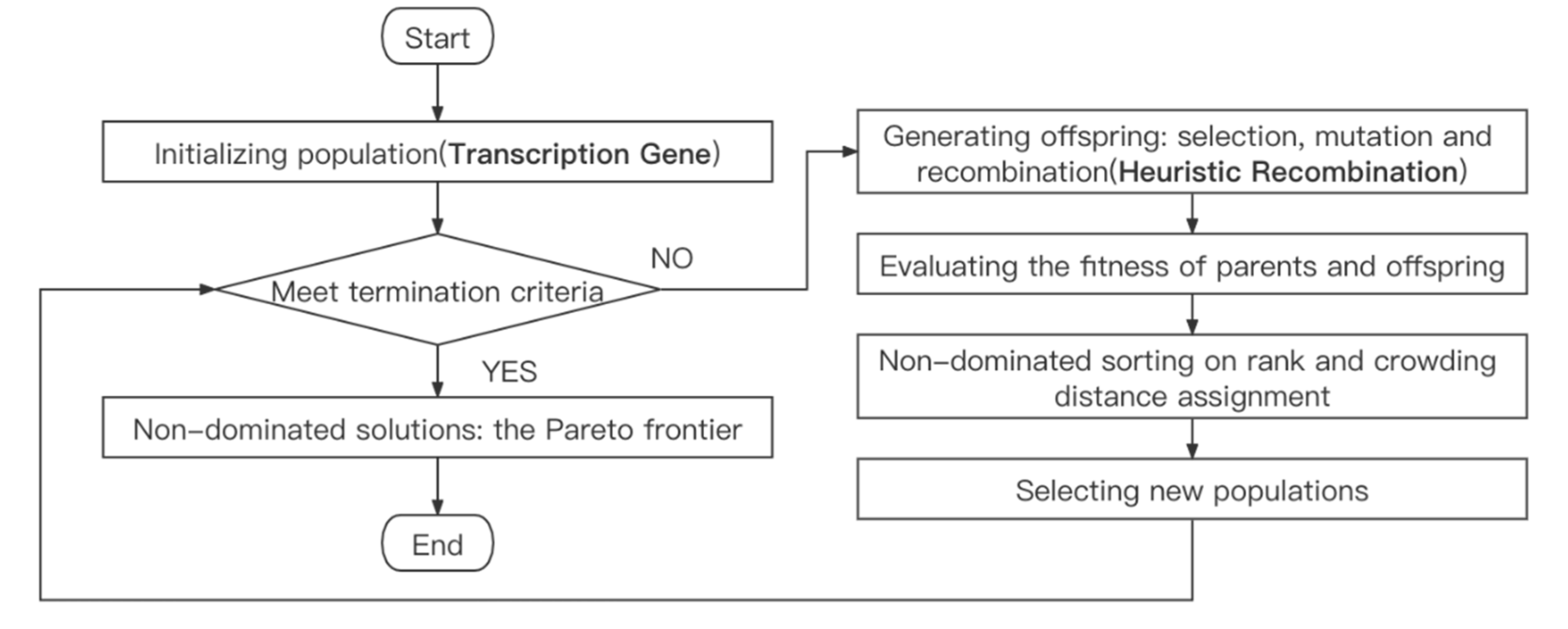
4.2. Improved NSGA2 Based on Transcription Gene and Heuristic Recombination (INSGA2-TGHR)

For how to solve multi-objective optimization problems, there are usually two ideas, one is to use mathematical planning methods to find the exact solution, and the other is to use intelligent computational methods to find the approximate solution. Since this problem is an extension of GQAP and has been proven to be an NP-hard problem, it will become unsolvable when the task and resource size increases, and also commonly used mathematical planning solvers such as gurobi [26] only support mixed integer linear programming and cannot solve quadratic planning problems. On the other hand, intelligent computing is commonly used in non-dominated sorting genetic algorithms (NSGA-II) [12], strength Pareto evolutionary algorithm II (SPEA2) [27], Pareto archival evolutionary strategy (PAES) [28] and multi-objective particle swarm optimization (MOPSO) [29], among which NSGA-II and its improvements performs better in finding a diverse set of solutions and in converging to near the true Pareto-optimal set compared with others [16]. For example, Ghasemi-Falavarjani et al. [17] used the benchmark NSGA-II algorithm to solve the time and energy bi-objective optimization problem in mobile cloud computing, M.A.B. Al-Tarawneh [18] took the application criticality and security as optimization objectives and modeled them as a bi-backpack problem using benchmark NSGA-II to solve, and Mahbuba Afrin [16] proposed Augmented NSGA-II to achieve good results in a multi-objective optimization problem for smart factory workflow resource allocation.

Therefore, for the IRMWAP problem, this work proposes the INSGA2-TGHR algorithm. This algorithm is a heuristic genetic algorithm that is redesigned based on NSGA-II, combining the previous ideas for solving GQAP and the workflow assignment problem. Figure 3 shows that when the monitor generates a RMW that needs to be offloaded, it will obtain the CEN resources information to run the INSGA2-TGHR and allocate computing resources to the tasks. As shown in Figure 4, Transcription Gene is used to create the initial population and Heuristic Recombination is used as a crossover operator to generate new offspring. The idea and detail of proposed algorithm will be discussed as follows:

4.2.1. Genetic Factors: Transcription Gene

In traditional genetic algorithms solving workflow assignment problems, all genetic operators are designed as integer arrays of task number length, where each gene made index symbolizes a specific task and gene refers to a specific resource, and matching tasks and resources by random assignment. This has the advantage of simplifying the relationship between tasks, resources, genes and fitness, but the problem is that the number of heterogeneous resources (monitors, edges, clouds) in CEN may not be equal, and then the probability of assigning tasks to different kinds of resources is also not equal. Therefore, the genetic factors are redesigned, and the concept of DNA transcription to generate RNA in biology is used here. “DNA”, a set of random real numbers of task length from 0 to N where N is the type of heterogeneous resources, will be generated first. Then, the “DNA” produces “RNA” by “transcription”. For example, a certain edge–cloud network (CEN) is composed of (6, 4, 2) heterogeneous resources, which has 6 local monitors, 4 edge servers, and 2 cloud servers and numbered sequentially from #1 to #12. A random real number “0.375402761769494”, its integer part “0”, corresponds to the 1st group (monitor), its fractional part “0.375402761769494” multiplied by the number of resources of the 1st group “6” and then rounded to “2”, corresponds to the third one, then its determined computing resources correspond to the third local monitors, #3. Similarly, a random real number “2.501432671965211” determined computing resource corresponds to the second cloud servers, #12, a random real number “1.5705781532276744” determined computing resource corresponds to the third edge servers, #9. the “RNA” is similar to traditional chromosome structure and can participate in evolution to produce offspring, as well as translate the allocation of resources and calculate fitness based on the encoding of genetic information. The “transcription” process divides the real numbers from 0 to N into an integer part and a decimal part, where the integer part determines the type of heterogeneous resources, and the decimal part determines the number of heterogeneous resources. The specific process is represented by Algorithm 1 and Figure 5, where “DNA” is a pre-obtained array, “Resource” is a dictionary nested array, the “Key” of the dictionary is the resource type and “Value” of the dictionary is an array of resource numbers of that type. In addition, the design of the genetic factors implicitly satisfies (3) (4), each subtask is assigned to only one computing resource.

Algorithm 1: Transcription

4.2.2. Mutation Operator

The mutation operator selects the swap mutation operator, and during mutation the mutation operator selects genes from inside the chromosome for mutation. The resource number with more occurrences inside the chromosome may correspond to the most suitable resource in the current environment, so the swap mutation has a higher probability of mutating a gene into these resources, thus increasing the concentration of resource usage and reducing the migration between subtasks. In addition, if the mutated new chromosome exceeds a certain resource limit, it will be eliminated later.

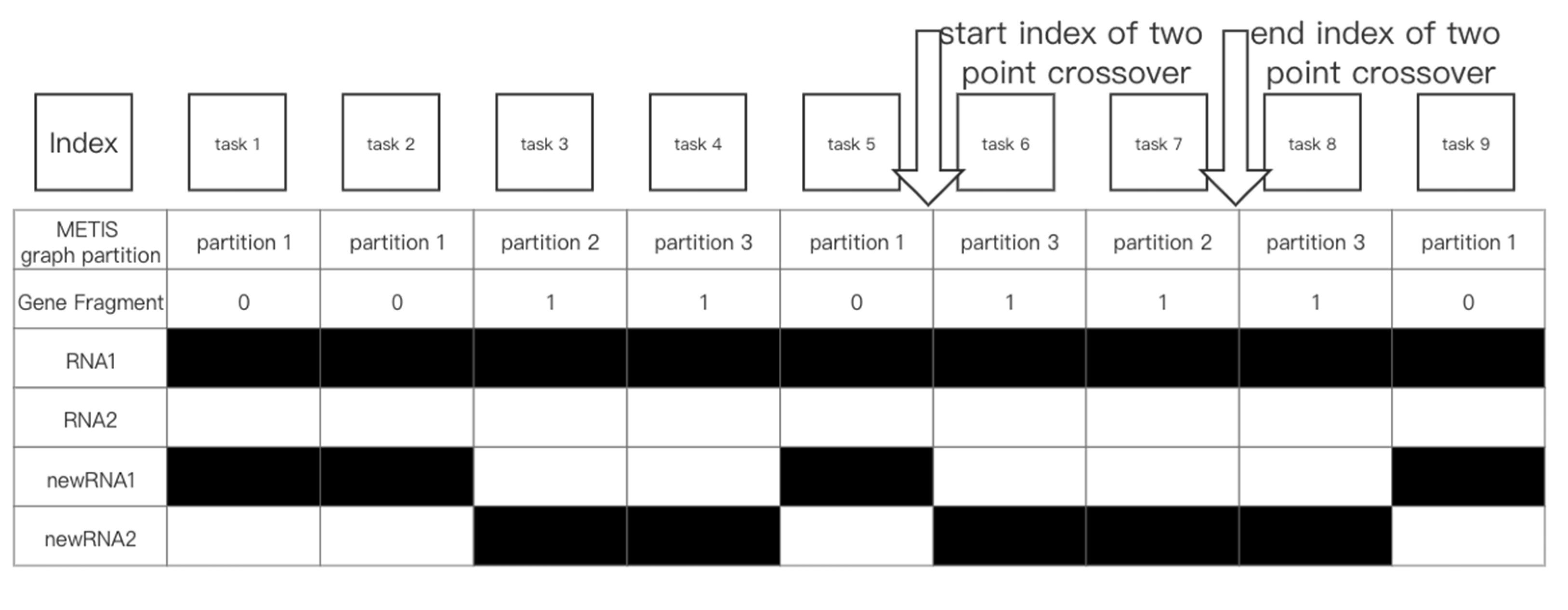
4.2.3. Crossover Operator: Heuristic Recombination

Two-point crossover refers to the random setting of two crossover points in the chromosomes of an individual followed by partial gene exchange. The specific procedure of the two-point crossover is: setting two random crossover points in the coding strings of two individuals paired with each other; exchanging the part of chromosomes of two individuals between the set two crossover points.

The recombination operator is a two-point crossover recombination operator based on the graph partitioning strategy, using the graph partitioning algorithm METIS [30] to group the workflows based on the amount of computation of subtasks in the workflow and the amount of data passed between subtasks. Each group consists of several subtasks, and the gene fragments corresponding to subtasks within the grouping are involved in the crossover as a whole when the recombination variation is performed. When subtasks are assigned to the same resource within a group, the data transfer between several subtasks takes place only in memory and does not involve network communication between computing resources, which effectively reduces the latency and cost of data transfer and thus exhibits a high degree of fitness, and this situation can be called “advantageous gene fragment”. For example, task A of data preprocessing is input-heavy and output-heavy, while task B of data feature extracting is input-heavy and output-light type, if these two tasks are executed sequentially on the same computing unit. The process of A’s output-heavy and B’s input-heavy only needs to be executed in the memory of that computing unit, without network transfer. This significantly reduces the transfer latency and bandwidth costs. The process of Heuristic Recombination is to use the graph partitioning algorithm to partition A and B tasks into the same group, forming an “advantageous gene fragment” as a whole for crossover recombination.

Then the “advantaged gene fragment” may be recombined to the new chromosome during the crossover process. If the entire new chromosome has a higher fitness, it will be reserved during the selection process. The “ordinary gene fragments” that are not assigned to the same resource may be replaced by “dominant gene fragments” in the process of crossover recombination, or may mutate in the process of mutation, and finally the algorithm will decide whether to reserve them for the next round of evolution according to the fitness.

The process is represented in Algorithm 2 and Figure 6, where the METIS [30] algorithm is used for graph partitioning, first, two crossover sites “x1” and “x2” are obtained, and the indexes of other genes consistent with the grouping within the sites are obtained according to the graph partitioning results. The above results were represented by the 0–1 array “col”. The recombined newRNA1 uses the gene of RNA1 on the index with “col” of 1 and the gene of RNA2 on the index with “col” of 0. newRNA2 is exactly the opposite.

Algorithm 2: Heuristic Double Point Recombination

4.2.4. Fitness Calculation

For the bi-objective optimization problem, the fitness functions for both optimization objectives latency and cost are defined and obey the conditions of (1) and (2), respectively. In addition, the genetic factors (5) and (6) that do not satisfy the constraints will be directly eliminated.

5. Experiments

In this section, experiments will analyze and compare the performance of the proposed bi-objective resource allocation algorithm by evolving generations, different types and numbers of tasks, different types and numbers of computing resources and the numbers of task instructions. The workflow in

Table 3. Experimental Parameters.

Params Type		Params Value
workflow	Number of subtasks	30–80
	instruction	10–800 MI
	memory	100–500 MB
	data dependency	10–100 kB
Local Monitor	CPU	0.8 Ghz*1
	memory	1 GB
	bandwidth	400 Mbps
Edge Server 1	CPU	3.0 Ghz*4
	memory	8 GB
	bandwidth	2 Gbps
	cost	2 RMB/h
Cloud Server 1	CPU	3.0 Ghz*8
	memory	16 GB
	bandwidth	4 Gbps
	cost	2 RMB/h
Local to Edge	cost	0.25 RMB/GB
	Latency	10 ms
Edge to Cloud	cost	0.75 RMB/GB
	Latency	30 ms
Local to Cloud	cost	1 RMB/GB
	Latency	40 ms

¹ Price reference is Huawei Cloud ECS and Huawei Cloud IEC [32].

is similar in structure to the motivational example in Figure 2, the quantification of its parameter instruction, memory, and data dependency are driven by real-world parameters (e.g., the runtime memory of the docker instance) and related references [15,18,31].

5.1. Simulation Environment

The experimental environment is based on python and geatpy [33], and the reference objectives are selected benchmark NSGA-II, INSGA2-TG(Transcription Gene) algorithm, INSGA2-HR(Heuristic Recombination) algorithm and extremums.

Table 4. Ablation of INSGA2-TGHR.

Algorithm	Initial Population	Mutation and Crossover Operator
Benchmark NSGA-II	random	simulated binary and polynomial mutation
INSGA2-TG	TG	simulated binary and polynomial mutation
INSGA2-HR	random	Swap and HR
INSGA2-TGHR	TG	Swap and HR

shows the Ablation of INSGA2-TGHR, where benchmark NSGA-II algorithm has a random initial population, using simulated binary crossover operator and polynomial mutation operator. INSGA2-TG has TG initial population, using simulated binary crossover operator and polynomial mutation operator, INSGA2-HR has random initial population, using swap mutation operator and HR crossover operator, INSGA2-TGHR has TG initial population, using swap mutation operator and HR crossover operator, and extremum of IRMWAP problem in both latency and cost directions are solved respectively by the gurobi [26].

Figure 7 compares the Pareto frontier of the four algorithms in the (6, 2, 1) resource setting, which has 6 local monitors, 2 edge servers and 1 cloud server. TGHR algorithm can obtain the solution closest to the extreme value and closer to the true Pareto frontier, and the convergence of its solution set is better than the other three algorithms. The TG algorithm is less exploratory than TGHR and HR, although it has a dominant initial population. The HR algorithm contains more monitor genes due to its initial gene population, so that its evolutionary direction will be more likely to favor the low-cost side. Benchmark NSGA-II algorithm does not reach convergence at 200 generations. It shows that the TG and HR algorithms have the advantage of dominant initial populations and evolutionary exploration, respectively, to find non-dominated solutions quickly and close to the Pareto frontier. In addition, the TGHR algorithm has the advantages of both TG and HR, and its solution set is balanced and closer to the real Pareto frontier.

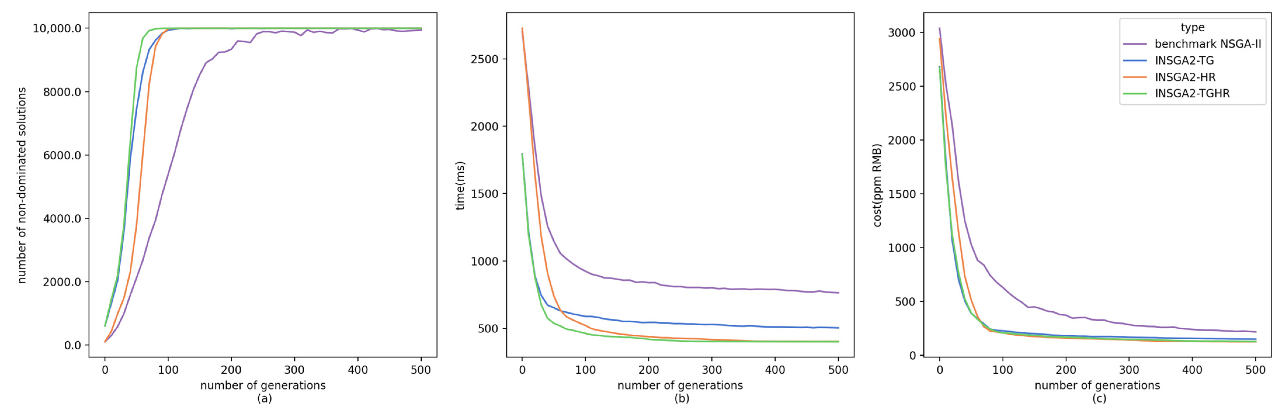
Impact of Evolution Generation

Figure 8 shows the impact of comparing the number of evolutionary generations of the four algorithms in the (6, 2, 1) resource setting.

The Figure 8a shows the number of non-dominated solutions, as shown in the figure, the TGHR algorithm works best and is the first to obtain close to 100 non-dominated solutions. The TG algorithm is second only to the TGHR algorithm, which is because both transcription gene can obtain more balanced random initial populations. The HR algorithm starts with a lower number of non-dominated solutions, but because the recombination operator of the HR algorithm is based on the variation of the dominant gene fragment, the non-dominated solutions are quickly viewed and retained. Benchmark NSGA-II algorithm is a purely random search, and the number of non-dominated solutions only approaches 100 when the number of iterations reaches 300, and there is some fluctuation after that.

The Figure 8b shows the average of the top 100 low-time solutions, and it can be seen that the TGHR algorithm works best, the HR algorithm is slower than TGHR, but it can still obtain high-quality low-time solutions by 200 generations by relying on the advantage of the HR. TG and Benchmark NSGA-II algorithms do not obtain solutions close to the extremes.

The Figure 8c is comparing the average of the top 100 low-cost solutions. TGHR and HR have relative performance, and HR is slightly better than TGHR because HR has a higher proportion of local genes, so it can find populations containing more local genes and achieve the effect of lower cost. TG algorithm finishes the population through iteration with the advantage of TG in the initial population is not superior. Benchmark NSGA-II algorithm starts to approach the extreme value at around 500 generations.

The TGHR algorithm combines the advantages of both TG and HR: the TG algorithm can obtain a dominant initial population, while the HR algorithm can quickly find and retain a dominant population. It can quickly obtain non-dominance by population advantage in the early evolutionary stage and can approach the extremum in about 100 generations by the recombination operator.

5.2. Impact of the Number of Resources

5.2.1. Impact of Local Resources

Figure 9a–d are comparing different resources in (4, 2, 1), (6, 2, 1), (8, 2, 1), (10, 2, 1) settings, respectively. As shown in the figure, the TGHR algorithm can obtain a more convergent Pareto front with a more balanced distribution under different resource conditions, while the HR algorithm has a solution set that is closer to the extreme value of low cost because its initial population contains more local monitor genes. TG algorithm has weaker convergence than TGHR algorithm and HR algorithm.

The box plot Figure 10 shows that as the number of local monitors increases, the solution set provided by the algorithm allocates more resources to the local monitors, thus leading to a slow decrease in cost and a slow increase in time as the number of local monitors increases. At the same time, it can be seen that the TGHR algorithm always finds the solution with the lowest time, and the HR algorithm tends to allocate more resources to the local monitor as the number of local monitors increases due to the characteristics of its initial population, which gives it an advantage in the direction of low cost.

5.2.2. Impact of Edge Resources

Figure 11a–d are comparing different resources in (6, 1, 1), (6, 2, 1), (6, 3, 1), (6, 4, 1) settings, respectively. From the figure, it can be seen that when there are fewer edge servers, the TGHR algorithm shows its unique advantage of better convergence of the solution set of the Pareto front to find the closest solution to the extreme value. The TG algorithm and HR algorithm in Figure 11a may fail to complete convergence in 200 generations of evolution due to the inability to find enough non-dominated solutions in the early stage of evolution.

The box plot Figure 12 shows that as the TGHR algorithm has stable performance. As the edge server resources increase, the tasks are assigned more on the edge server with higher computational efficiency, so (6, 2, 1) has lower minimum time than (6, 1, 1). However, when the edge resources become abundant and all computational tasks will be offloaded to the edge servers, the minimum time is no longer reduced. As the edge resources increase, the proportion of edge genes in the initial population of the TGHR algorithm increases, and therefore, it no longer has the advantage of low-cost. This can show that the TGHR algorithm is less affected by the change of resource allocation and can perform more stable performance.

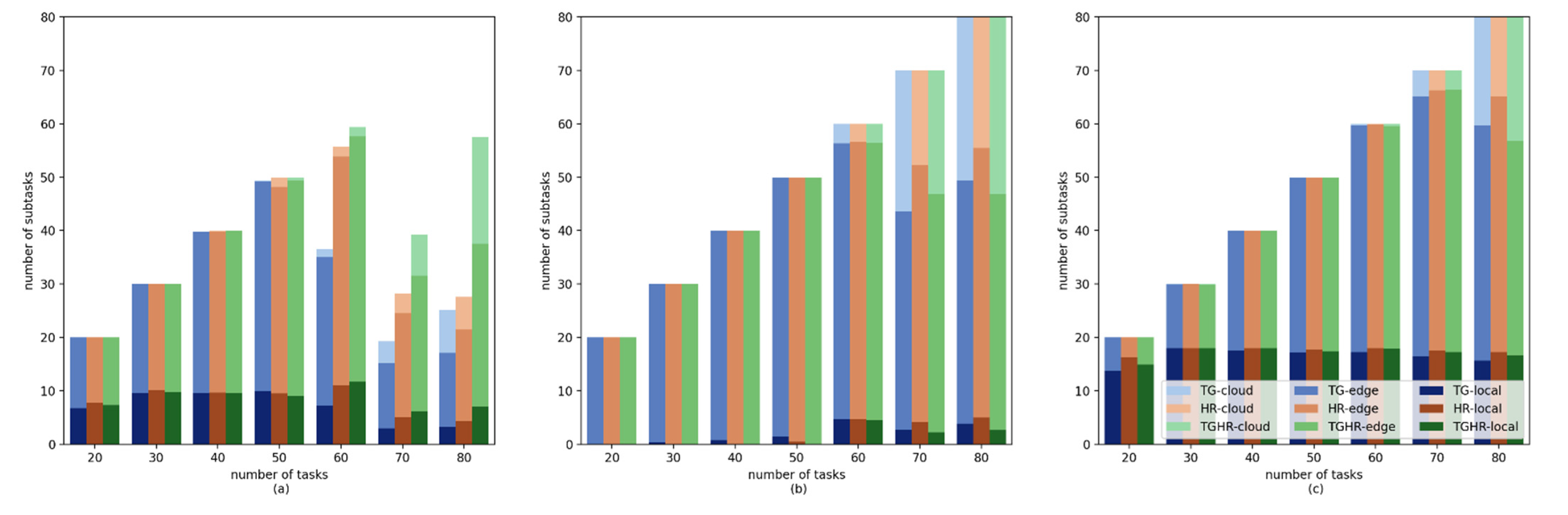
5.3. Impact of the Number of Subtasks

Figure 13 compares the allocation ratio of tasks executed monitor, edge, and cloud for a workflow containing 20 to 80 tasks, and each task occupies 300 M of memory, in (6, 2, 1) resources setting.

Figure 13a shows the allocation ratio in all Pareto fronts, and the number of local runs in the figure is relatively smooth. As the number of tasks continues to increase, the algorithm gradually assigns tasks to the cloud as the system approaches the edge server operating load. As the number of subtasks increases, when the number of subtasks exceeds 60, the 200 generations evolution starts to unable to meet the demand, and the performance of the TG algorithm starts to degrade and cannot find the non-dominated solution corresponding to the number of populations, and when the number of tasks exceeds 70, all algorithms cannot find the non-dominated solution corresponding to the number of populations. However, it can be seen that the performance of the TGHR algorithm is still the best, and the number of non-dominated solutions found is much more than that of the TG algorithm and the HR algorithm. The figure also shows that the performance of the HR algorithm is slightly better than that of the TG algorithm, which is due to the fact that the HR algorithm speeds up the speed of finding non-dominated solutions.

Figure 13b,c shows the allocation ratio in 100 solutions near low-time and near low-cost in the solution set, respectively. There will always be fewer local machines using low performance in low-time, and as the number of tasks increases, more and more tasks will be allocated in the cloud, gradually reaching a one-to-one ratio of resources on the edge–cloud. As many tasks as possible in low-cost will be assigned first in local monitor, and the maximum capacity of running tasks that local can provide is 18, and the figure has basically approached the maximum load of the local monitor.

From Figure 14, it can be seen that the TGHR algorithm always finds the solution with the lowest time, and the HR algorithm can find the solution with the lowest cost in some cases, which is due to the fact that the initial population of the HR algorithm has more genes representing the assignment to the local, and it can find the non-dominated solution with low cost faster, but its comprehensive performance is not as good as that of the TGHR algorithm.

5.4. Impact of the Number of Task Instructions

Figure 15 compares the impact of the number of instructions for different tasks. Where each workflow contains 30 tasks (subtasks), each task occupies 300 M of memory, and the number of instructions to be executed for each task is 50 to 900, in (6, 2, 1) resources setting. It shows that the TGHR algorithm is more sensitive to the number of instructions of subtasks. As the number of instructions of tasks increases, the advantage of cloud side of high-performance computing is emphasized, and the TGHR algorithm reduces the assignment of tasks available at the edge side and assigns more tasks to the cloud side.

Figure 15a shows the allocation ratio in all Pareto fronts. It indicates that the share of cloud server increases as the number of instructions increases, due to the fast speed of cloud computing, whose less computation time offsets the impact of bandwidth latency. Figure 15b,c shows the allocation ratio in 100 solutions near low-time and near low-cost in the solution set, respectively. It can be seen that the low-time strategy is more sensitive to time, and low-performance local monitors are not used, while the share of cloud servers with high computational speed increases rapidly. On the contrary, the low-cost strategy is more sensitive to price and basically keeps the local monitors running at full load. The share of cloud servers also increases slowly with the number of task instructions.

As shown in Figure 16, because of the lower number of subtasks, almost all algorithms find low-time and low-cost extremes. HR algorithm has a slightly larger low-time minimum solution than others, which is because its initial population has more local monitor genes and thus fewer edge and cloud genes obtained by evolution. The performance of TGHR algorithm is also more robust as seen in the figure. Starting from instruction number 350, the advantages of cloud computing start to reveal, so the average time of the Pareto frontier for the three algorithms decreases and the average cost increases.

5.5. Results and Discussions

The ablation experiments show that TG can produce a more balanced initial population, HR can accelerate the iteration efficiency. The INSGA2-TGHR algorithm has the advantages of both, and it can find the non-dominated solution set quickly and keep approaching the true Pareto front through evolution. Its performance is stable, and it can find suitable allocation schemes among different types and numbers of computing resources.

6. Conclusions and Future Directions

In this paper, we design a local edge–cloud industrial robot-monitoring system (IRMS) architecture, define the Industrial Robot-Monitoring Workflow Resource Allocation Problem (IRMWAP), and propose an improved NSGA-II algorithm (INSGA2-TGHR) based on the characteristics of IRMSs, using workflows to accomplish industrial robot-monitoring tasks. The experimental results show that the INSGA2-TGHR algorithm has a more balanced initial population and can retain the “dominant gene fragment” in the evolutionary iterations to quickly obtain a non-dominated solution set and a more convergent Pareto frontier through evolutionary iterations, and its Pareto frontier obtains time minima and cost minima that are 4.66% and 15.52% more accurate than benchmark NSGA-II’s respectively in 200 generations. The performance of INSGA2-TGHR algorithm is stable on different types and number of computing resources sets, sensitive to the number of instructions of the tasks, and able to offload computationally intensive tasks to more clouds.

In future work, we plan to further validate and extend the applicability of this algorithm in IRMSs. In this paper, we only consider the monitoring of fixed-position industrial robots; but in real industrial factory scenarios, there are also mobile robots involved in activities, and their network environments may include various environments such as Bluetooth, Wi-Fi, and 5G. Therefore, such working conditions as mobility and complex network environment are still the direction of future research. In addition, how the monitor itself can make autonomous decisions and choose the appropriate solution in the Pareto frontier through artificial intelligence algorithms is also a problem to be considered in the future.

References

1. Chen, Y.; Dong, F. Robot Machining: Recent Development and Future Research Issues. Int. J. Adv. Manuf. Technol. 2013, 66, 1489–1497. [Google Scholar] [CrossRef] [Green Version]
2. Hou, Z.; Chen, J. Research Review of Remote Monitoring and Fault Diagnosis of Industrial Robots. Mach. Tool Hydraul. 2018, 46, 172–176, 168. [Google Scholar]
3. Yang, H.; Sun, Z.; Jiang, G.; Zhao, F.; Lu, X.; Mei, X. Cloud-Manufacturing-Based Condition Monitoring Platform With 5G and Standard Information Model. IEEE Internet Things J. 2021, 8, 6940–6948. [Google Scholar] [CrossRef]
4. Atmoko, R.A.; Yang, D. Online Monitoring & Controlling Industrial Arm Robot Using MQTT Protocol. In Proceedings of the 2018 IEEE International Conference on Robotics, Biomimetics, and Intelligent Computational Systems (Robionetics), Bandung, Indonesia, 8–10 August 2018; pp. 12–16. [Google Scholar] [CrossRef]
5. Chen, W.; Yaguchi, Y.; Naruse, K.; Watanobe, Y.; Nakamura, K.; Ogawa, J. A Study of Robotic Cooperation in Cloud Robotics: Architecture and Challenges. IEEE Access 2018, 6, 36662–36682. [Google Scholar] [CrossRef]
6. Hu, G.; Tay, W.; Wen, Y. Cloud Robotics: Architecture, Challenges and Applications. IEEE Network 2012, 26, 21–28. [Google Scholar] [CrossRef]
7. Kehoe, B.; Patil, S.; Abbeel, P.; Goldberg, K. A Survey of Research on Cloud Robotics and Automation. IEEE Trans. Automat. Sci. Eng. 2015, 12, 398–409. [Google Scholar] [CrossRef]
8. Wan, J.; Tang, S.; Yan, H.; Li, D.; Wang, S.; Vasilakos, A.V. Cloud Robotics: Current Status and Open Issues. IEEE Access 2016, 4, 2797–2807. [Google Scholar] [CrossRef]
9. O’Donovan, P.; Leahy, K.; Bruton, K.; O’Sullivan, D.T.J. An Industrial Big Data Pipeline for Data-Driven Analytics Maintenance Applications in Large-Scale Smart Manufacturing Facilities. J. Big Data 2015, 2, 25. [Google Scholar] [CrossRef] [Green Version]
10. Cloud Edge Computing: Beyond the Data Center. OpenStack Is Open Source Software for Creating Private and Public Clouds. Available online: https://www.openstack.org/use-cases/edge-computing/cloud-edge-computing-beyond-the-data-center/?lang=en_US (accessed on 24 September 2021).
11. Pan, Y.; Er, M.J.; Li, X.; Yu, H.; Gouriveau, R. Machine Health Condition Prediction via Online Dynamic Fuzzy Neural Networks. Eng. Appl. Artif. Intell. 2014, 35, 105–113. [Google Scholar] [CrossRef]
12. Deb, K.; Pratap, A.; Agarwal, S.; Meyarivan, T. A Fast and Elitist Multiobjective Genetic Algorithm: NSGA-II. IEEE Trans. Evol. Computat. 2002, 6, 182–197. [Google Scholar] [CrossRef] [Green Version]
13. Xuhong, M.; Zhizeng, L. The Design and Implement of Embedded Remote Control System in Industrial Robot. In Proceedings of the 2012 International Conference on Computer Science and Electronics Engineering, Hangzhou, China, 23–25 March 2012; pp. 332–335. [Google Scholar] [CrossRef]
14. Yin, H.L.; Wang, Y.M.; Xiao, N.F.; Jiang, Y.R. Real-Time Remote Manipulation and Monitoring Architecture of an Industry Robot. In Proceedings of the 2008 IEEE International Joint Conference on Neural Networks (IEEE World Congress on Computational Intelligence), Hong Kong, China, 1–8 June 2008; pp. 1228–1234. [Google Scholar] [CrossRef]
15. Chen, W.; Yaguchi, Y.; Naruse, K.; Watanobe, Y.; Nakamura, K. QoS-Aware Robotic Streaming Workflow Allocation in Cloud Robotics Systems. IEEE Trans. Serv. Comput. 2021, 14, 544–558. [Google Scholar] [CrossRef]
16. Afrin, M.; Jin, J.; Rahman, A.; Tian, Y.-C.; Kulkarni, A. Multi-Objective Resource Allocation for Edge Cloud Based Robotic Workflow in Smart Factory. Future Gener. Comput. Syst. 2019, 97, 119–130. [Google Scholar] [CrossRef]
17. Ghasemi-Falavarjani, S.; Nematbakhsh, M.; Shahgholi Ghahfarokhi, B. Context-Aware Multi-Objective Resource Allocation in Mobile Cloud. Comput. Electr. Eng. 2015, 44, 218–240. [Google Scholar] [CrossRef]
18. Al-Tarawneh, M.A.B. Bi-Objective Optimization of Application Placement in Fog Computing Environments. J. Ambient. Intell. Hum. Comput. 2021. [Google Scholar] [CrossRef]
19. Rahman, A.; Jin, J.; Cricenti, A.; Rahman, A.; Panda, M. Motion and Connectivity Aware Offloading in Cloud Robotics via Genetic Algorithm. In Proceedings of the GLOBECOM 2017-2017 IEEE Global Communications Conference, Singapore, 4–8 December 2017; pp. 1–6. [Google Scholar] [CrossRef]
20. Xie, Y.; Guo, Y.; Mi, Z.; Yang, Y.; Obaidat, M.S. Loosely Coupled Cloud Robotic Framework for QoS-Driven Resource Allocation-Based Web Service Composition. IEEE Syst. J. 2020, 14, 1245–1256. [Google Scholar] [CrossRef]
21. Li, S.; Zheng, Z.; Chen, W.; Zheng, Z.; Wang, J. Latency-Aware Task Assignment and Scheduling in Collaborative Cloud Robotic Systems. In Proceedings of the 2018 IEEE 11th International Conference on Cloud Computing (CLOUD), San Francisco, CA, USA, 2–7 July 2018; pp. 65–72. [Google Scholar] [CrossRef]
22. Hirsch, M.; Mateos, C.; Zunino, A.; Majchrzak, T.A.; Grønli, T.-M.; Kaindl, H. A Task Execution Scheme for Dew Computing with State-of-the-Art Smartphones. Electronics 2021, 10, 2006. [Google Scholar] [CrossRef]
23. Sanabria, P.; Tapia, T.F.; Neyem, A.; Benedetto, J.I.; Hirsch, M.; Mateos, C.; Zunino, A. New Heuristics for Scheduling and Distributing Jobs under Hybrid Dew Computing Environments. Wirel. Commun. Mobile Comput. 2021, 2021, 8899660. [Google Scholar] [CrossRef]
24. Pallasch, C.; Wein, S.; Hoffmann, N.; Obdenbusch, M.; Buchner, T.; Waltl, J.; Brecher, C. Edge Powered Industrial Control: Concept for Combining Cloud and Automation Technologies. In Proceedings of the 2018 IEEE International Conference on Edge Computing (EDGE), San Francisco, CA, USA, 2–7 July 2018; pp. 130–134. [Google Scholar] [CrossRef]
25. Hahn, P.M.; Kim, B.-J.; Guignard, M.; Smith, J.M.; Zhu, Y.-R. An Algorithm for the Generalized Quadratic Assignment Problem. Comput. Optim. Appl. 2008, 40, 351–372. [Google Scholar] [CrossRef] [Green Version]
26. Gurobi. The Fastest Solver—Gurobi. Available online: https://www.gurobi.com/ (accessed on 24 September 2021).
27. Zitzler, E.; Laumanns, M.; Thiele, L. SPEA2: Improving the Strength Pareto Evolutionary Algorithm. TIK-Rep. 2001. [Google Scholar] [CrossRef]
28. Knowles, J.; Corne, D. The Pareto Archived Evolution Strategy: A New Baseline Algorithm for Pareto Multiobjective Optimisation. In Proceedings of the Proceedings of the 1999 Congress on Evolutionary Computation-CEC99 (Cat. No. 99TH8406), Washington, DC, USA, 6–9 July 1999; pp. 98–105. [Google Scholar] [CrossRef]
29. Coello Coello, C.A.; Lechuga, M.S. MOPSO: A Proposal for Multiple Objective Particle Swarm Optimization. In Proceedings of the Proceedings of the 2002 Congress on Evolutionary Computation, CEC’02 (Cat. No.02TH8600), Honolulu, HI, USA, 12–17 May 2002; Volume 2, pp. 1051–1056. [Google Scholar] [CrossRef]
30. Karypis, G.; Kumar, V. A Fast and High Quality Multilevel Scheme for Partitioning Irregular Graphs. SIAM J. Sci. Comput. 1998, 20, 359–392. [Google Scholar] [CrossRef]
31. He, S.; Lyu, X.; Ni, W.; Tian, H.; Liu, R.P.; Hossain, E. Virtual Service Placement for Edge Computing Under Finite Memory and Bandwidth. IEEE Trans. Commun. 2020, 68, 7702–7718. [Google Scholar] [CrossRef]
32. Price Calculator. HUAWEI CLOUD. Available online: https://www.huaweicloud.com/pricing.html (accessed on 24 September 2021).
33. Geatpy: The Genetic and Evolutionary Algorithm Toolbox with High Performance in Python. Available online: http://www.geatpy.com/ (accessed on 24 September 2021).
Figure 1. IRMS Edge–Cloud Architecture.
Applsci 11 10066 g001
Figure 2. Motivating example: comprehensive assessment workflow.
Applsci 11 10066 g002
Figure 3. Trigger mechanism flow chart for INSGA2-TGHR.
Applsci 11 10066 g003
Figure 4. Flow chart of INSGA2-TGHR.
Applsci 11 10066 g004
Figure 5. DNA Transcription RNA.
Applsci 11 10066 g005
Figure 6. Process of Heuristic Recombination.
Applsci 11 10066 g006
Figure 7. Comparison of Pareto frontier. (a) Comparison of four algorithms; (b) Comparison of TGHR and benchmark NSGA-II; (c) Comparison of TGHR and TG; (d) Comparison of a and TGHR and HR.
Applsci 11 10066 g007
Figure 8. Comparison of evolution generations. (a) The relationship between evolutionary generations and non-dominant solutions; (b) The relationship between evolutionary generations and low-time Extremum; (c) The relationship between evolutionary generations and low-cost Extremum.
Applsci 11 10066 g008
Figure 9. The Pareto frontier in different local resources setting. (a), (b), (c), (d) are comparing different resources in (4, 2, 1), (6, 2, 1), (8, 2, 1), (10, 2, 1) settings, respectively.
Applsci 11 10066 g009
Figure 10. The boxplot in different local resources setting. (a) Comparing the effect of local resources setting on time; (b) Comparing the effect of local resources setting on cost. The rhombus symbols represent outliers, which are also the same in Figure 12, Figure 14 and Figure 16 in the later text.
Applsci 11 10066 g010
Figure 11. The Pareto frontier in different edge resources setting. (a), (b), (c), (d) are comparing different resources in (6, 1, 1), (6, 2, 1), (6, 3, 1), (6, 4, 1) settings, respectively.
Applsci 11 10066 g011
Figure 12. The boxplot in different edge resources setting. (a) Comparing the effect of edge resources setting on time; (b) Comparing the effect of edge resources setting on cost.
Applsci 11 10066 g012
Figure 13. Allocation ratio of resource in different number of tasks. (a) Allocation ratio of resource in all Pareto fronts; (b) Allocation ratio of resource in near low-time 100 solutions; (c) Ratio of resource in near low-cost 100 solutions.
Applsci 11 10066 g013
Figure 14. The boxplot in different number of tasks. (a) Comparing the effect of number of tasks on time; (b) Comparing the effect of number of tasks on cost.
Applsci 11 10066 g014
Figure 15. Allocation ratio of resource in different number of task instructions. (a) Allocation ratio of resource in all Pareto fronts; (b) Ratio of resource in near low-time 100 solutions; (c) Allocation ratio of resource in near low-cost 100 solutions.
Applsci 11 10066 g015
Figure 16. The boxplot in different number of task instructions. (a) Comparing the effect of number of task instructions on time; (b) Comparing the effect of number of task instructions on cost.
Applsci 11 10066 g016