Abstract
With the surge of motor vehicle ownership and land intensification, plenty of large parking lots emerge as the times demand. Although it solves the problem of insufficient parking spaces, it intensifies the interaction between dynamic and static traffic. This paper presented an impact assessment method for the interaction of dynamic and static traffic flow in parking lots. Firstly, the average vehicle delay was selected as the evaluation index. The delay effect caused by the interaction of dynamic and static traffic flow was determined according to the driving path of vehicles. Then, the average vehicle delay models of arrival vehicles, departure vehicles, and road vehicles in the parking lot were established. Finally, for the parameters difficult to determine directly in the delay model, this paper proposed a method to calibrate the model parameters by using the simulation experimental data on the VISSIM platform. The results showed that the errors of the three models are within the controllable range, and the delay model parameters had high reliability and feasibility. The delay models can provide a quantitative basis for the parking lot management department to formulate regulation strategies and realize more refined information guidance and navigation in the parking lot.
1. Introduction
With the surge of urban development density, the trend of land intensification is obvious, such as large commercial complexes, large hospitals, industrial parks, and other buildings and facilities came into being, giving birth to a large number of large parking lots. Although increasing the number of parking spaces in large parking lots can alleviate the shortage of parking spaces, it makes the arrival and departure of vehicles more concentrated. This leads to a more obvious impact on the dynamic and static traffic between the parking lot and the surrounding roads, which leads to a series of new problems of “parking difficulty”, such as the bottleneck between the entrance and exit of the parking lot and the connecting road. This is not only directly related to the accessibility of vehicles, but also leads to the problem of slow traffic or congestion on the connecting roads, which reduces the traffic efficiency of the surrounding road network. Based on the above analysis, the problem of traffic congestion at the junction of entrance and exit of large parking lots is outstanding. It is particularly important to make a good connection between static traffic and dynamic traffic at the entrance and exit of large parking lots. How to evaluate the influence of dynamic and static traffic at the entrance and exit of large parking lots needs further analysis and research.
At present, the impact analysis of dynamic and static traffic is mostly focused on signal intersections, expressways and urban roads. A method based on vehicle dynamics theory was proposed to calculate vehicle delay and queue length through floating vehicle survey data [1,2]. An impact assessment method based on queuing time to study traffic congestion at signalized intersections was studied, and the relationship between queuing time, queuing length and vehicle delay was discussed [3,4,5]. Nannan used the queue length and traffic efficiency index of the intersection to evaluate the safety of the interaction between traffic flows at the intersection [6,7,8,9]. In these studies, delay, queue length, parking times and density are mainly used as indicators of traffic impact analysis to identify and predict the congestion of traffic flow. The research contents are more inclined to the analysis of the impact on the dynamic traffic.
For the researches of parking lots, it is mostly through the construction of simulation environment to obtain the index results such as queue length, delay and speed, and then conduct impact analysis. Based on VISSIM, Xiaojun Yue and other scholars [10,11] compared the different design schemes of the parking lot and analyzed the impact between the dynamic and static traffic flow of the parking lot with the queue length as the evaluation index. Jiang Qiu selected sections with similar road conditions and traffic conditions as the research object, further studied the relationship between the traffic flow at the entrance and exit of the parking lot and the road running speed, and studied the interaction between the traffic flow at the entrance and exit of the parking lot and the road traffic [12,13]. At present, although there are many studies on the connection of parking lots, the interaction between vehicles entering and leaving the parking lot and road vehicles is still lacking. In addition, the relationship between traffic volumes and evaluation indexes is not directly revealed, which makes the models are complex and difficult to understand.
Considering the interaction between the entrance and exit channels of the parking lot and the connecting road, this paper proposed a dynamic and static traffic impact analysis method of the parking lot based on the vehicle delay model. As the vehicle delay can effectively reflect the congestion degree of dynamic traffic flow and the perception sensitivity of static traffic flow, this paper selected the average vehicle delay as the evaluation index of the impact between the traffic flows at the entrance and exit of large parking lots. According to the driving routes, vehicles were divided into arriving vehicles in the parking lot, departing vehicles in the parking lot and road vehicles. Then, the delay models of these three types of vehicles were established, respectively. Finally, the parameters of the model were calibrated on the VISSIM platform by using the simulation data.
The organizational structure of this study is as follows: Section 2 constructs the delay models of vehicles arriving in parking lots, vehicles leaving parking lots and road vehicles. Section 3 uses the VISSIM platform to complete the parameter calibration of the vehicle delay models. Section 4 verifies the accuracy and reliability of the vehicle delay model through case analysis. The conclusion is given in Section 5.
2. Establishment of Vehicle Delay Model
2.1. Overview of Delay Indicators
There are many evaluation indicators describing traffic impact [14], such as queue length, delay, and traffic capacity. Vehicle delay can not only reflect the congestion severity, fuel consumption, and travel time loss of dynamic traffic flow but also measure the rationality and reliability of traffic channelization design. At the same time, drivers are most sensitive to the change of time when queuing in congestion. In addition, vehicle delay is widely used in traffic congestion evaluation, intersection signal control, and route guidance. Considering that delay is quite significant for dynamic traffic and static traffic, this paper selected the average vehicle delay as the evaluation index of dynamic and static traffic impact analysis of parking lot.
Vehicle delay refers to the difference between the actual travel time of the vehicle and the travel time under the ideal state [15]. Generally, it includes fixed delay, operation delay, parking delay, and queuing delay.
2.2. Establishment of Delay Model
To better study the relationship between dynamic and static traffic at the entrance and exit of parking lots, this paper made some assumptions and tests on the delay model to reduce the influence of accidental factors.
(1) Vehicles can pass smoothly after passing through the downstream intersection without queuing. Therefore, it will not affect the operation of road vehicles in this section.
(2) The entry lane of vehicles at the exit of the parking lot is the first lane closest to the entrance and exit, and there will be no driving behaviors of crossing the traffic flow.
(3) When the vehicles arriving at the parking lot queue at the entrance gate, the queuing vehicles will not spread to the road and cause delay to the road. At the same time, the vehicles can find the berth smoothly after passing the gate, and there will be no queue in the parking lot.
(4) There will be no pedestrians passing through the road near the entrance and exit of the parking lot, no parking behaviors of vehicles loading and unloading passengers, and no arrival and parking behavior of buses. It is to highlight the interference of vehicles at the entrance and exit of the parking lot to road vehicles.
(5) The entrance and exit gates of the parking lot are single-channel services.
The dynamic and static traffic flow of the parking lot is divided into arrival vehicles, departure vehicles, and road vehicles according to the vehicle driving path. Based on the above assumptions, vehicle delay models are established respectively.
2.2.1. Delay Model of Arriving Vehicle
The driving process of vehicles arriving at the parking lot is as follows. First, the vehicle waits for an acceptable gap from the second lane to decelerate into the entrance channel or decelerates from the first lane to enter the entrance channel, and then the vehicle decelerates in front of the gate and stops, waiting for the rod to be lifted and accelerated through. The delay of arriving vehicles is shown in Figure 1.
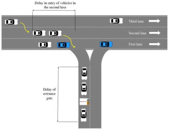
Figure 1.
Delay of Arriving Vehicles.
It can be seen from the above driving process that the delay of arriving vehicles mainly includes the following.
(1) Fixed delay . It is the acceleration and deceleration delays caused by the geometric size of the entrance channel and the channelization method at the connection between the entrance and the connecting road.
(2) Delay of entrance gates . It is the acceleration, deceleration, and queue delay when passing through the parking lot gate. Because the entrance and exit of the parking lot is a single channel queuing system, the M/M/1 queuing model is adopted. According to the model [16], it can be deduced that the time of vehicles in the queuing system is the average delay time of vehicles, as shown in Equation (1).
where is the average delay of vehicles arriving at the parking lot, and is the number of vehicles arriving at the parking lot, and is the service rate of the entrance gate.
(3) Delay of second lane vehicles entering the parking lot . It is the acceleration and deceleration delay and queuing delay caused by vehicles in the second lane (starting from the right) passing through the first lane (close to the entrance channel) to enter the entrance channel.
The first lane is regarded as the main road and the second lane is regarded as the secondary road. Only when the headway of the vehicles on the main road is greater than the critical gap, the vehicles on the secondary road are allowed to enter the conflict area.
Based on the above assumptions, Harders [17] gave a formula for calculating the average delay of secondary road vehicles. Since the capacity of the second lane is affected by the width of the first lane, the geometric characteristics of the entrance, and other factors, it is necessary to correct the capacity of vehicles in the second lane when crossing the first lane. Finally, the average delay of vehicles in the second lane when entering the parking lot can be obtained. As shown in Equation (2).
where is the average delay of vehicles entering the parking lot in the second lane, and is the number of vehicles entering the parking lot in the first lane, and is the number of vehicles entering the parking lot in the second lane, and is the traffic volume of the first lane, and is the critical gap for arriving vehicles in the second lane, and is the following time of the arriving vehicle in the second lane, and is the correction factor for the capacity of vehicles in the second lane when crossing the first lane.
Therefore, the average delay of arriving vehicles in the parking lot is shown in Equation (3).
where is the average delay of vehicles arriving at the parking lot, and is the fixed delay of vehicles arriving at the parking lot, and is the average delay of arriving vehicles passing through the entrance gate, and is the average delay of vehicles entering the parking lot in the second lane, and is the number of vehicles arriving at the parking lot, and is the number of vehicles entering the parking lot in the second lane, and is the number of lanes.
2.2.2. Delay Model of Leaving Vehicle
The driving process of vehicles leaving the parking lot is as follows. The vehicle decelerates or stops in front of the gate, waits for the pole to be lifted and accelerates through, then seeks acceptable clearance and decelerates into the road, and finally accelerates away. The delay caused by leaving the vehicle is shown in Figure 2.
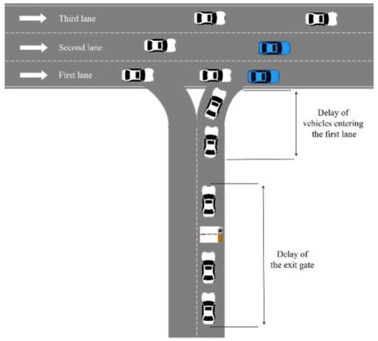
Figure 2.
Delay of Leaving Vehicles.
It can be seen from the above driving process that the vehicles leaving the parking lot are also affected by the fixed delay , the delay of the exit gate , and the delay of leaving the vehicles and driving into the road .
(1) Delay of the exit gate [16].
where is the average delay of leaving vehicles passing through the exit gate, and is the service rate of the export gate, and is the number of vehicles leaving the parking lot.
(2) Delay of vehicles leaving the parking lot to enter the first lane of the road .
The first lane is regarded as the main road, and the exit channel of the parking lot is regarded as the secondary road. Based on the delay formula [17], the capacity of vehicles leaving the parking lot to drive into the first lane is corrected. Finally, the average delay of vehicles leaving the parking lot and driving into the first lane of the road is obtained, as shown in Equation (5).
where is the average delay of vehicles leaving the parking lot and driving into the first lane of the road, and is the number of vehicles leaving the parking lot, and is the traffic volume of the first lane, and is the critical gap between the parking lot and the first lane of the road, and is the following time of vehicles leaving the parking lot, and is the capacity correction factor for vehicles leaving the parking lot and driving into the first lane.
Therefore, the average delay of vehicles leaving the parking lot is shown in Equation (6).
where is the average delay of vehicles leaving the parking lot, and is the fixed delay of vehicles leaving the parking lot, and is the average delay of leaving vehicles passing through the exit gate, and is the average delay of leaving the vehicle into the first lane of the road.
2.2.3. Delay Model of Road Vehicle
In practice, road vehicles, vehicles leaving the parking lot, and vehicles arriving at the parking lot do not fully follow the principle of main road priority, and road vehicles will also be delayed.
The delay of road vehicles can be analyzed according to the number of lanes. The number of lanes refers to the total number of lanes conforming to the right-in and right-out organization mode at the entrance and exit of the parking lot.
Through the field investigation of parking lots with more than 300 parking spaces and more than two entrances and exits in Nanjing. The results showed that the entrance and exit connecting roads of the parking lot are mainly two lanes, three lanes, and four lanes on the same side. Because the first and the second lane close to the entrance and exit are often selected for vehicles arriving and leaving the parking lot, the third and the fourth lanes on the same side have less impact on dynamic and static traffic [18,19,20,21]. Therefore, this paper mainly studied the roads with two and three lanes on the same side.
In the case of three lanes on the same side, vehicles in the second lane can continue to pass through the third lane by changing lanes, so only vehicles in the first lane will delay. The delays in the first lane are as follows.
(1) Delay in the first lane affected by vehicles leaving the parking lot .
where is the average delay of vehicles in the first lane affected by vehicles leaving the parking lot, and is the number of vehicles leaving the parking lot, and is the number of vehicles in the first lane affected by vehicles leaving the parking lot, and is the following time of road vehicles in the first lane, and is the critical gap between the entry and exit conflict zone of vehicles in the first lane, and is the following time of vehicles in the first lane entering and exiting the conflict zone, and is the capacity correction factor for the first lane entering and exiting the conflict zone.
(2) Delay in the first lane affected by passage vehicles of the second lane
where is the average delay of vehicles in the first lane affected by the passage vehicles of the second lane, and is the traffic volume of the first lane, and is the number of vehicles in the first lane affected by vehicles in the second lane, and is the number of vehicles entering the parking lot in the second lane, and is the critical gap between the vehicles in the first lane and the conflict zone passed by the vehicles in the second lane, and is the following time when the vehicle in the first lane enters the conflict zone passed by the vehicle in the second lane, and is the following time of road vehicles in the first lane, and is the capacity correction factor of the conflict zone between the first lane and the second lane.
The delay caused by road vehicles in three lanes on the same side was shown in Figure 3.
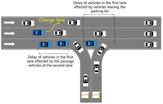
Figure 3.
Delay of Road Vehicles in Three Lanes on the Same Side.
In the case of two lanes on the same side, the vehicles in the first lane are still affected by the vehicles leaving the parking lot and the vehicles passing through the second lane. However, vehicles in the second lane cannot change lanes, so they need to queue up for vehicles in front of the same lane to enter the parking lot, which will lead to queue delays. The queuing delay of the second lane is about equal to the average delay of the second lane vehicles entering the parking lot, as shown in Equation (9).
where is the traffic volume of the first lane, and is the number of vehicles entering the parking lot in the first lane, and is the number of vehicles entering the parking lot in the second lane, and is the following time of vehicles arriving in the second lane, and is the critical clearance of vehicles arriving in the second lanes, and is the capacity correction factor for vehicles in the second lane crossing the first lane.
Therefore, the average delay of road vehicles is shown in Equation (10).
where is the average delay of road vehicles, and is the average delay of vehicles in the first lane affected by vehicles leaving the parking lot, and is the average delay of vehicles in the first lane passing through the second lane, and is the queue delay of vehicles in the second lane waiting for vehicles in front to find an acceptable gap to enter the parking lot, and is the total traffic volume of the road, and is the traffic volume of the first lane, and is the traffic volume of the second lane, and is the number of lanes.
The notations and descriptions of all formulas were systematically listed in Table A3 in Appendix C.
3. Parameter Calibration of Vehicle Delay Model
The direct determination of the parameters in the above delay model is a very complex task because it is affected by many factors, most of which are uncertain and inaccurate. At present, mainstream delay models such as the Webster model [22], the Miller model [7], the HCM 2000 model [23] mainly calibrate parameters indirectly through the data collected by traditional detectors. However, the data collected by the traditional detector has the disadvantages of poor reliability and low comprehensiveness, and it is not real-time, resulting in a large gap between the results and the actual situation. Moreover, it cannot handle many variables and interactions defined in the model in this paper. However, the simulation experiment has strong repeatability and can realize the simulation of large samples and multiple scenes. By setting the simulation environment, the simulation effect can be very close to the real situation. Therefore, this paper proposed to use the simulation experimental data calibration method to determine the parameters of the delay model, and finally got the vehicle delay value.
Due to the complete driving behavior model and fine facility description of the VISSIM platform, it can better restore the characteristics of facilities and make the simulation effect closer to reality. At the same time, several interfaces are provided for secondary development. Therefore, VISSIM was selected as the parameter calibration platform of the delay model in this paper. The vehicle delay is obtained by inputting traffic volume and other data, and the calibration of model parameters would be completed.
The specific steps of the simulation experiment data calibration method are as follows.
Step 1: Obtain the basic data required for simulation scene modeling. It mainly includes road data, entrance, and exit channel data, and driving path ratio data.
(1) Road data. It includes the number of lanes connecting the road, lane width, lane design speed, and section length.
(2) Parking ramp/ Entrance and exit channel data. It includes the geometric dimension data of the entrance and exit channel, the angle between the entrance and exit and the connecting road, the position of the gate in the entrance and exit channel, the average time for vehicles to pass through the gate, the average time for vehicles to leave through the gate, the speed for vehicles to pass through the entrance without road vehicle interference and the speed for vehicles to leave through the exit.
(3) Travel proportion data. It includes the proportion of entering the parking lot from different lanes and the proportion of driving into different lanes from the parking lot during peak hours.
Step 2: Build a simulation scene. Build the road network scene in the simulation software, and set the attributes of road section parameters, entrances and exits, deceleration zone, and so on.
Step 3: Correct the parameters of the simulation software. The headway [24] is used to correct the parameters of the car following the model in VISSIM, making the simulation animation closer to the real traffic operation and increasing the authenticity and reliability of the simulation. The basic principle of parameter correction is to input different parameter combinations to minimize the difference between the headway distribution of simulation output and that of field investigation. Because PSO (Particle Swarm Optimization) has the advantages of memory, no crossover and mutation operation, and fast convergence speed, PSO was used for correction in this paper.
Step 4: Set the detector. Set up travel time detectors for road vehicles, arrival vehicles, and departure vehicles in the parking lot.
Step 5: Calculate the average delay of the simulation vehicle. Input the traffic volume combinations of various types of vehicles and run the simulation experiment and monitor the delay of each vehicle. Firstly, calculate the average delay of all traffic volume combinations under a random seed. And then calculate the average delay of all traffic volume combinations under all random seeds, which is the required average delay of final simulated vehicles.
Step 6: Batch simulation. This paper used VISSIM’s COM interface for secondary development through external programming to realize batch simulation and reduce repetitive and cumbersome work.
Step 7: Calibrate the delay model parameters. The mathematical analysis software is used to calibrate the delay model parameters. The parameter calibration can be characterized by R-square [25]. The value range of R-square is [0,1]. The closer it is to 1, the better the calibration effect. It is generally considered that R-square is greater than 0.9, and the calibration value is accepted.
4. Analysis of Simulation Experiment
4.1. Establishment of Simulation Model
Jingfeng parking lot in Nanjing mainly serves the parking demand of Jingfeng commercial plaza. There are three floors in the parking lot, namely B1, B2, and B3. Its total number of berths is 1800. The interaction between dynamic and static traffic is quite intense.
There are two entrances and exits in the parking lot. The entrance and exit on the east side are connected to the branch with two lanes on the same side. It belongs to the entrance and exit of the atypical parking lot. The road connecting the west entrance and exit is three lanes on the same side, and the entrance and exit are 155 m away from the downstream T-shaped intersection. There are few conflict points at the intersection, and there is no traffic control, and the traffic capacity of the road is high. It can be concluded that the entrance and exit of the West parking lot are suitable for dynamic and static traffic impact analysis. Therefore, this paper selected the west entrance as the research object.
(1) Obtain the basic data required for simulation scene modeling
After pre-investigation, it was found that the peak time is 17:00–19:00. The video survey method and manual survey method were used to obtain the data such as the entrance, the geometric size of the road and the proportion of vehicles entering the parking lot in each lane, so as to provide data support for the simulation scene.
The traffic flow entering the parking lot and the traffic flow of the branch road were counted at an interval of 15 min. The statistical results were shown in Table A1 in Appendix A. It can be seen that the proportion of vehicles arriving at the parking lot to the number of road vehicles fluctuates around 20%;
Similarly, conduct a traffic volume survey on the connecting road of the west exit. The statistical results were shown in Table A2 in Appendix B. The results showed that the path ratio from the second lane to the parking lot was 1:1. In addition, only a few vehicles entered from the third lane, which was negligible compared with the number of vehicles entering from the other two lanes.
(2) Construct the VISSIM simulation scene of the Jingfeng parking lot
Input the road network scene, the attributes of the road section, entrances and exits, deceleration zone and other parameters in VISSIM simulation software.
(3) Correct the parameters of the VISSIM simulation software
This paper used the headway index [24] to correct the parameters of the car-following model, so that the simulation experiment was closer to the actual situation. The iterative process was shown in Figure 4. After 11 iterations, the objective function suddenly decreased and then tended to be flat, indicating that the value of the objective function at this time gradually approaches the optimal solution after updated calculation and met the convergence conditions. The final objective function value is 0.1467 s. The average headway obtained from the experiment was 5.2652 s. Since the measured headway was 5.4119 s, the relative error can be calculated as 2.71%. The error is within the control range, which means that the optimal solution was obtained.
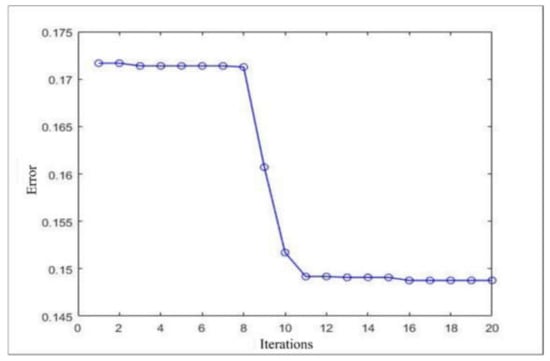
Figure 4.
Iterative process and error value.
Therefore, the three parameters of the car-following model in VISSIM were modified. The average parking distance was changed to 1.8654m. The additional part of the safety distance was changed to 1.5643. The multiple of safety distance was changed to 2.5795.
(4) Set parameter information such as conflict area, stop signal, signal lamp and travel time detector.
The built simulation environment is shown in Figure 5.
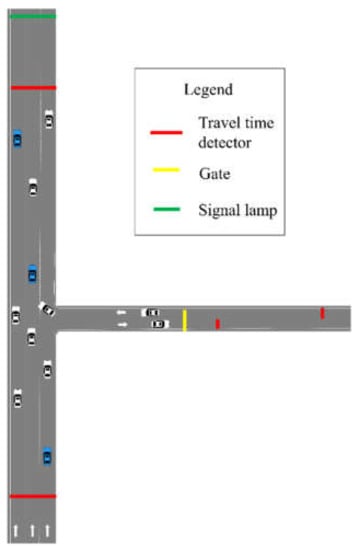
Figure 5.
Final simulation environment of West entrance.
(5) Run the simulation model and conduct batch simulation
Input the traffic volume of different combinations according to the traffic volume of investigation and statistics. Enter the number of vehicles from 200 to 2100 vehicles/h in the road traffic volume, and increase the traffic flow with an interval of 100 vehicles/h. It was a total of 20 traffic flows. Input 30 to 315 veh/h for vehicles leaving, and increase the traffic flow with an interval of 15veh/h. It was a total of 20 traffic flows. Therefore, there are 400 input combinations. There were 10 random seeds, and a total of 4000 simulation experiments were required. Finally, run the program for batch simulation.
The average delay of the simulated vehicle was calculated by using the simulation data. Then the simulated vehicle delay and the number of vehicles of each type were substituted into the established vehicle average delay model. Then use the fitting toolbox [26] in MATLAB to calibrate the unknown parameters in the model.
4.2. Analysis of Simulation Results
(1) Arriving vehicles
After fitting, the parameter calibration results of the average delay model of arriving vehicles in the parking lot were shown in Table 1.

Table 1.
Calibration Results of Delay Model Parameters of Arriving Vehicles.
The R-square of the model was 0.9379. It is generally believed that when R-square is greater than 0.9, the fitting effect is good [26]. Therefore, this paper accepted the parameter calibration results. Substitute the parameter calibration results into Equation (3) to obtain Equation (11), and then the average delay model of arriving vehicles at the west entrance of Jingfeng parking lot during peak hours can be obtained.
(2) Leaving vehicles
After fitting, the parameter calibration results of the average delay model of leaving vehicles in the parking lot were shown in Table 2.
Table 2.
Calibration Results of Delay Model Parameters of Leaving Vehicles.
The R-square of the model is 0.9478, indicating that the fitting effect was good. Therefore, this paper accepted the parameter calibration results. Substitute the parameter calibration results into Equation (6) to obtain Equation (12), and then the average delay model of vehicles leaving the west entrance of Jingfeng parking lot during peak hours.
(3) Road vehicles
After fitting, the parameter calibration results of the average delay model of road vehicles were shown in Table 3.
Table 3.
Calibration Results of Delay Model Parameters of Road Vehicles.
The R-square of the model is 0.9457, indicating that the fitting effect was good. Therefore, this paper accepted the parameter calibration results. Substitute the parameter calibration results into Equation (11) to obtain Equation (13), and then the average delay model of road vehicles near the west entrance of Jingfeng parking lot during peak hours can be obtained.
4.3. Analysis of Simulation Results
To test the accuracy of the model and parameter calibration, this paper investigated the traffic conditions at the west entrance and exit of the Jingfeng parking lot on a new day and obtained the number of vehicles of various types and the actual delay time.
The number of vehicles observed was substituted into the delay model (Equations (11)–(13)), then the average delay of vehicles was calculated, and the error was analyzed with the measured data to test the effect of the model. The calculation results were shown in Table 4.
Table 4.
Evaluation of Delay Model.
It can be seen from the above table that the relative error of the delay of arriving vehicles is 5.49%, and the relative error of the delay time of leaving vehicles is 4.45%, which means the errors are within the control range. It can be concluded that the delay model of arriving and leaving vehicles has high accuracy, practicability, and reliability. For the delay model of road vehicles, although the relative error is large, the absolute error of the two is small, and the absolute error is 0.57 s. Therefore, it can also be determined that the model can better calculate the average delay of road vehicles.
5. Conclusions
Plenty of large parking lots can solve the problem of insufficient parking spaces, but it intensifies the interaction between dynamic and static traffic. This paper proposed a dynamic and static traffic impact analysis method of the parking lot. Firstly, the average vehicle delay was selected as the evaluation index. The average vehicle delay models of arrival vehicles, departure vehicles and road vehicles were established. Then, for the parameters difficult to determine directly, this paper proposed a method to calibrate the model parameters by using the simulation experimental data on the VISSIM platform. Finally, the delay model is verified by the Jingfeng parking lot.
The delay models proposed in this paper reveal a direct relation between traffic volume and vehicle delay. The delay of dynamic and static traffic flow in the parking lot calculated by models can provide a reference for predicting whether there is congestion between the parking lot and the connecting road, which is beneficial for the management department to guide and navigate in advance and improves the operational efficiency of the parking lots and connecting roads.
There were still limitations in this paper. For example, this paper selected the typical scene of the entrance and exit of the parking lot to build the vehicle delay models. In the future, the dynamic and static traffic impact under atypical scenarios can be further studied and can be compared with the research in typical scenarios.
Author Contributions
Conceptualization, L.W. and J.C. (Jun Chen); methodology, L.W.; software, L.W. And X.C.; validation, J.C. (Jian Chen) and C.Z.; formal analysis, L.W.; investigation, J.C. (Jun Chen); resources, X.C.; data curation, C.Z.; writing—original draft preparation, L.W.; writing—review and editing, J.C. (Jun Chen) and C.Z.; visualization, J.C. (Jian Chen). All authors have read and agreed to the published version of the manuscript.
Funding
This research was funded by the National Natural Science Foundation of China (Grant No.719701059), and The Key Project of Transportation Science and Technology Achievement & Transformation of Jiangsu Province (Grant No.2019Z01), and the Research Planning Fund for Humanities and Social Sciences of the Ministry of Education(Grant No.19YJAZH011) and SEU Postdoc Grant(Grant No.2242020R20026).
Institutional Review Board Statement
Not applicable.
Informed Consent Statement
Not applicable.
Data Availability Statement
The raw data used in this study are available from the corresponding author on request.
Conflicts of Interest
The authors declare no conflict of interest.
Appendix A
Table A1.
Proportion of vehicles arriving at the parking lot to the number of road vehicles.
Table A1.
Proportion of vehicles arriving at the parking lot to the number of road vehicles.
| Time | Vehicles Arriving at the Parking Lot | Road Vehicles | Proportion |
|---|---|---|---|
| 17:00–17:15 | 55 | 276 | 19.93% |
| 17:15–17:30 | 58 | 289 | 20.07% |
| 17:30–17:45 | 65 | 323 | 20.12% |
| 17:45–18:00 | 62 | 312 | 19.87% |
| 18:00–18:15 | 46 | 228 | 20.18% |
| 18:30–18:45 | 40 | 201 | 19.90% |
| 18:45–19:00 | 43 | 216 | 19.91% |
| Total | 414 | 2069 | 20.01% |
Appendix B
Table A2.
Proportional data of driving path.
Table A2.
Proportional data of driving path.
| Time | Total Leaving Vehicles | Vehicles Entering the Rightmost Lane (Vehicles) | Vehicles Entering Other Lanes (Vehicles) |
|---|---|---|---|
| 17:00–17:15 | 37 | 36 | 1 |
| 17:15–17:30 | 38 | 38 | 0 |
| 17:30–17:45 | 40 | 39 | 1 |
| 17:45–18:00 | 42 | 40 | 2 |
| 18:00–18:15 | 36 | 36 | 0 |
| 18:15–18:30 | 33 | 32 | 1 |
| 18:30–18:45 | 34 | 33 | 1 |
| 18:45–19:00 | 38 | 38 | 0 |
| Total | 298 | 292 | 6 |
Appendix C
Table A3.
Notations table.
Table A3.
Notations table.
| Symbol | Description | Unit |
|---|---|---|
| The average delay of vehicles arriving at the parking lot | s | |
| The acceleration and deceleration delays caused by the geometric size of the entrance channel and the channelization method at the connection between the entrance and the connecting road. | s | |
| The acceleration, deceleration, and queue delay when passing through the parking lot gate | s | |
| The average delay of vehicles entering the parking lot in the second lane | s | |
| The average delay of vehicles leaving the parking lot | s | |
| The average delay of leaving vehicles passing through the exit gate | s | |
| The average delay of vehicles leaving the parking lot and driving into the first lane of the road | s | |
| The fixed delay of vehicles leaving the parking lot | s | |
| The average delay of road vehicles | s | |
| The average delay of vehicles in the first lane affected by vehicles leaving the parking lot | s | |
| The average delay of vehicles in the first lane affected by the passage vehicles of the second lane | s | |
| The queue delay of vehicles in the second lane waiting for vehicles in front to find an acceptable gap to enter the parking lot | s | |
| The number of vehicles arriving at the parking lot | veh/h | |
| The number of vehicles entering the parking lot in the first lane | veh/h | |
| The number of vehicles entering the parking lot in the second lane | veh/h | |
| The total traffic volume of the road | veh/h | |
| The traffic volume of the first lane | veh/h | |
| The traffic volume of the second lane | veh/h | |
| The number of vehicles leaving the parking lot | veh/h | |
| The number of vehicles in the first lane affected by vehicles leaving the parking lot | veh/h | |
| The number of vehicles in the first lane affected by vehicles in the second lane | veh/h | |
| The critical gap between the parking lot and the first lane of the road | s | |
| the following time of vehicles leaving the parking lot | s | |
| The following time of road vehicles in the first lane | s | |
| The critical gap for arriving vehicles in the second lane | s | |
| the following time of the arriving vehicle in the second lane | s | |
| The critical gap between the entry and exit conflict zone of vehicles in the first lane | s | |
| The following time of vehicles in the first lane entering and exiting the conflict zone | s | |
| The critical gap between the vehicles in the first lane and the conflict zone passed by the vehicles in the second lane | s | |
| The following time when the vehicle in the first lane enters the conflict zone passed by the vehicle in the second lane | s | |
| The capacity correction factor for the first lane entering and exiting the conflict zone | - | |
| the capacity correction factor for vehicles leaving the parking lot and driving into the first lane | - | |
| The correction factor for the capacity of vehicles in the second lane when crossing the first lane | - | |
| The capacity correction factor of the conflict zone between the first lane and the second lane | - | |
| The service rate of the entrance gate. | s−1 | |
| The service rate of the export gate | s−1 | |
| The number of lanes | - |
References
- Tolami, S.; Mehran, B.; Hellinga, B. Delay and Queue Length Estimation at Signalized Intersections Using Archived Automatic Vehicle Location and Passenger Count Data from Transit Vehicles. In Proceedings of the Transportation Research Board 94th Annual Meeting, Washington DC, USA, 11–15 January 2015. [Google Scholar]
- Cetin, M. Estimating Queue Dynamics at Signalized Intersections from Probe Vehicle Data: Methodology Based on Kinematic Wave Model. Transp. Res. Rec. 2012, 2315, 164–172. [Google Scholar] [CrossRef] [Green Version]
- Li, B.; Cheng, W.; Li, L. Real-Time Prediction of Lane-Based Queue Lengths for Signalized Intersections. J. Adv. Transp. 2018, 2018, 5020518. [Google Scholar] [CrossRef] [Green Version]
- Ermagun, A.; Levinson, D. Spatiotemporal traffic forecasting: Review and proposed directions. Transp. Rev. 2018, 38, 786–814. [Google Scholar] [CrossRef]
- Gu, J.; Fu, Q.; Hu, J. Traffic Congestion Status Evaluation for Signal-controlled Intersection Based on Queuing Time Index. J. Transp. Inf. Saf. 2020, 38, 80–86. [Google Scholar]
- Sun, X.; Lin, K.; Jiao, P.; Lu, H. The Dynamical Decision Model of Intersection Congestion Based on Risk Identification. Sustainability 2020, 12, 5923. [Google Scholar] [CrossRef]
- Hao, N.; Feng, Y.; Zhang, K.; Tian, G.; Zhang, L.; Jia, H. Evaluation of traffic congestion degree: An integrated approach. Int. J. Distrib. Sens. Netw. 2017, 13, 155014771772316. [Google Scholar]
- Memon, I.; Mirza, H.T.; Arain, Q.A.; Memon, H. Multiple mix zones de-correlation trajectory privacy model for road network. Telecommun. Syst. 2019, 70, 557–582. [Google Scholar] [CrossRef]
- Yu, Z.; Huang, L.; Li, X.; Li, B.; Zou, B. Queueing Process Sensing and Prediction at Intersection Based on Video. J. Transp. Syst. Eng. Inf. Technol. 2020, 20, 33–39. [Google Scholar]
- Yue, X.; Wang, C. Analysis of entrance and exit csapacity of underground parking lot in commercial plaza. J. Shandong Jiaotong Univ. 2018, 26, 26–31. [Google Scholar]
- Feng, Z.; Zhang, L.; Xu, Y.; Zhang, J. Planning and design method of parking lot entrance and exit based on microscopic simulation. J. North China Univ. Sci. Technol. (Nat. Sci. Ed.) 2018, 40, 73–77. [Google Scholar]
- Qiu, J.; Huang, Z.; Pan, J. Empirical Analysis on Traffic Impact of Project Entrance and Exit Based on Big Data. Sci. Technol. Innov. 2018, 28, 99–101. [Google Scholar]
- Ma, Z.; Xu, A.; Shao, Y. Study on Entrance and Exit Setting of Underground Parking Lot in wanda plaza of Xining City. Qinghai Technol. 2019, 26, 33–36. [Google Scholar]
- Schwanz, A. Developing Static and Dynamic Multimodal Transportation System Models to Estimate Individual Commuter Footprints Using ArcGIS, Google Maps and Here360. Ph.D. Thesis, California State University, Fresno, CA, USA, 2017. [Google Scholar]
- Sun, X.; Feng, S. Research on the Influence of Bus Stop Time on Intersection Delay Based on VISSIM Simulation. J. Chongqing Jiaotong Univ. (Nat. Sci. Ed.) 2019, 38, 97–101. [Google Scholar]
- Tang, J. Queuing Theory and Its Application; Science Press: Beijing, China, 2016. [Google Scholar]
- Wang, D. Traffic Flow Theory; China Communications Press: Beijing, China, 2002. [Google Scholar]
- Min-Allah, N.; Qureshi, M.B.; Alrashed, S.; Rana, O.F. Cost efficient resource allocation for real-time tasks in embedded systems. Sustain. Cities Soc. 2019, 48, 101523. [Google Scholar] [CrossRef]
- Khan, S.U.; Min-Allah, N. A goal programming based energy efficient resource allocation in data centers. J. Supercomput. 2012, 61, 502–519. [Google Scholar] [CrossRef]
- Lyu, Y.; Chen, L.; Zhang, C.; Qu, D.; Min-Allah, N.; Wang, Y. An interleaved depth-first search method for the linear optimization problem with disjunctive constraints. J. Glob. Optim. 2018, 70, 737–756. [Google Scholar] [CrossRef]
- Min-Allah, N.; Khan, S.U.; Yongji, W. Optimal task execution times for periodic tasks using nonlinear constrained optimization. J. Supercomput. 2012, 59, 1120–1138. [Google Scholar] [CrossRef]
- Fuzzy model of vehicle delay to determine the level of service of two-lane roads. Expert Syst. Appl. 2016, 54, 48–60. [CrossRef]
- Liu, Z.; Xu, C.; Chen, L.; Zhou, S. Dynamic Traffic Flow Entropy Calculation Based on Vehicle Spacing. IOP Conf. Ser. Earth Environ. Sci. 2019, 252, 052073. [Google Scholar] [CrossRef]
- Kan, Y.; Meng, F. A Simulation Parameter Correction System Design Based on the Measured Data. In Proceedings of the International Conference on Computational Intelligence & Communication Networks, Mathura, India, 27–29 September 2013. [Google Scholar]
- Liu, S. Mathematical Statistics Theory, Method, Application and Software Calculation; Huazhong University of Science & Technology Press: Wuhan, China, 2005. [Google Scholar]
- Hu, Q. Using MATLAB curve fitting toolbox to do curve fitting. Comput. Knowl. Technol. 2010, 6, 5822–5823. [Google Scholar]
Publisher’s Note: MDPI stays neutral with regard to jurisdictional claims in published maps and institutional affiliations. |
© 2021 by the authors. Licensee MDPI, Basel, Switzerland. This article is an open access article distributed under the terms and conditions of the Creative Commons Attribution (CC BY) license (https://creativecommons.org/licenses/by/4.0/).