Coupled Numerical Method for Modeling Propped Fracture Behavior

Featured Application

A potential application of our coupled numerical model is the better understanding of propped fracture dynamics which may result in a more efficient fracturing treatment design for engineers working in the upstream division of the petroleum industry.

Abstract

Hydraulic fracturing is a well-known production intensification technique in the petroleum industry that aims to enhance the productivity of a well drilled mostly in less permeable reservoirs. The process’s effectiveness depends on the achieved fracture conductivity, the product of fracture width, and the permeability of the proppant pack placed within the fracture. This article presents an innovative method developed by our research activity that incorporates the benefit of the Discrete—and Finite Element Method to describe the in situ behavior of hydraulic fractures with a particular emphasis on fracture conductivity. DEM (Discrete Element Method) provided the application of random particle generation and non-uniform proppant placement. We also used FEM (Finite Element Method) Static Structural module to simulate the elastic behavior of solid materials: proppant and formation, while CFD (Computational Fluid Dynamics) module was applied to represent fluid dynamics within the propped fracture. The results of our numerical model were compared to data of API RP-19D and API RP-61 laboratory measurements and findings gained by publishers dealing with propped fracture conductivity. The match of the outcomes verified the method and encouraged us to describe proppant deformation and embedment and their effect as precisely as possible. Based on the results, we performed sensitivity analysis which pointed out the impact of several factors affecting proppant embedment, deformation, and fracture conductivity and let one be aware of a reasonable interpretation of propped hydraulic fracture operation. However, DEM–CFD coupled models were introduced regarding fracturing before, to the best of our knowledge, the developed workflow of coupling DEM–FEM–CFD for modeling proppant-supported fracture behavior has not been applied yet, thus arising new perspectives for explorers and engineers.

1. Introduction

Hydraulic fracturing is a stimulation treatment widely used in the upstream division of the petroleum industry to enhance well productivity in tight gas/oil or shale gas/oil reservoirs [1]. The purpose of fracturing is production intensification by creating high conductive, propped fractures that provide a larger inflow surface than the cylindrical area of an ordinary well [2]. The fracturing procedure is controlled on the surface and executed by high-power hydraulic pumps boosting the hydraulic fluid to exceed the formation breakdown pressure at the bottom hole. This pressure of the hydraulic fluid initiates the formation to break. Meanwhile, the fracture starts to propagate according to the petrophysical properties of the given formation. Proppant is a granular media with high porosity, is mixed with the fracturing fluid to prop the fracture and prevent formation closure that would result in an ineffective stimulation [3]. The phenomenon investigated in this research occurs after fractures are created, and hydraulic pumps are stopped entailing the hydraulic fluid pressure to drop below the formation closure pressure. At this point, there is no more extra pressure energy to hold the fractures open, which leads to a closing action of the formation, which is prevented by proppant particles that carry the stresses of formation closure [4]. The primary indicator, which characterizes the fracturing treatment, is the fracture conductivity calculated as the product of fracture width and proppant pack permeability. Since the above-described situation affects fracture conductivity significantly, it is crucial to model the problem comprehensively.

Several earlier studies deal with proppant embedment; Huitt and McGlothlin [5] derived an equation based on the knowledge of proppant concentration and overburden load to compute proppant embedment. It is a semi-empirical model containing two characteristic constants, which could be determined by fitting the results with experimental data. They performed relevant experiments to prove the capability of this equation, and they found that proppant embedment is a more relevant phenomenon than proppant crush under formation pressure. The factors affecting proppant embedment were determined by the formation’s competency, the proppant’s size, the concentration of the proppant, and the overburden pressure. They concluded that a stiffer, tougher material would be a better propping agent than sand because sand would crush rather than embed under the overburden pressure.

Volk et al. [6] derived empirical equations based on experimental data to determine the parameters influencing proppant embedment, such as proppant concentration, size, distribution, rock type, etc.

Lacy et al. [7] carried out experimental research on proppant embedment in non-tight reservoir cores; therefore, the results can be interpreted as limited ones. Nevertheless, the results showed that the most critical factors that have a relevant impact on proppant embedment were closure pressure, proppant size, and fluid properties. Therefore, Lacy et al. [8] also developed a computer-controlled measurement that determined propped-fracture width and proppant embedment as a function of closure pressure, the concentration of proppant paving, proppant size, core mechanical characteristics, etc.

Guo and Liu [9] investigated the proppant embedment in core samples experimentally. They also found that the fracture width could be remarkably reduced because of the proppant embedment, especially in soft formations. They examined the experimental data of proppant embedment at different conditions, and they published empirical equations that can determine the proppant embedment as a function of formation pressure, the elastic modulus of the core, and proppant concentration.

Further experimental studies of proppant embedment and fracture conductivity were published by many researchers [10,11,12,13,14]. However, these empirical or semi-empirical solutions could provide interpretations in limited conditions. Others [15,16,17,18] also conducted experimental research about fracture conductivity. However, the exactness of these developed models considering the prediction of in situ fracture behavior may not be satisfactory due to the artificial conditions from which they have been derived.

The lack of a comprehensive analytical model was fulfilled by Li et al. [19], who developed an analytical approach based on the Hertzian Contact Theory to investigate the effect of proppant deformation and embedment on fracture conductivity. Their research was derived from two mutually squeezed spheres and considered only mathematical and physical principles; therefore, it was found to be a valuable method to gain information about conductivity influencing factors. Their approach could provide results for proppant embedment, change in fracture aperture, deformation, permeability, and conductivity for single- and multi-layer patterns. Furthermore, their equations are completely analytical, resulting in an elegant solution for fracture behavior modeling. However, it also has limitation because some random factors, like non-regular proppant shape, uneven proppant placement, uneven stress distribution, and complicated fracture geometry, cannot be described analytically.

After all, it can be stated that the detailed description of a propped fracture behavior requires a numerical solution due to the random character of the phenomenon. Therefore, a few numerical approaches have already been developed. For example, Sun et al. [20] investigated the impact of high-quality proppant on fracture conductivity and long-term production. They created a numerical model based on field case studies, and the result showed that upgrading the completion design with a high resistant proppant enhanced the production enormously.

Fan et al. [21] investigated hydraulic fracture conductivity by creating a coupled numerical model using Particle Flow Code (PFC), which is a three-dimensional discontinuum mechanics simulator, and the lattice Boltzmann (LB) method to solve the Navier–Stokes equations. In addition, the effect of proppant concentration in the fracture and effective stress was investigated, and they found the partial monolayer pattern with large-diameter proppants as an alternative to improve fracture conductivity.

Zhang et al. [22] developed a DEM–CFD numerical modeling process to examine proppant embedment and fracture conductivity after hydraulic fracturing in shale formations. They concluded shale hydration as the main reason for proppant embedment. They also found that conductivity increases with proppant concentration and size and decreases with closure pressure.

Fan et al. [23] also conducted experimental and numerical research on fracture conductivity in narrow fractures. They used laboratory experiments and a numerical modeling approach that combines continuum mechanics, the discrete element method, and the lattice Boltzmann (LB) method. Their results showed a strong correlation between proppant embedment and rock mechanical properties. However, the results are related to narrow fractures only, characterized mainly by monolayer proppant pattern.

Zhu et al. [24] examined a reasonably new fracturing technique called channel fracturing. The essence of channel fracturing is promoting the hydrocarbon-bearing rock stable voids by intermittent proppant pumping and mixing fibers to the fracking fluid. These voids serve as high conductive areas within the proppant pack to improve the oil transport into the well. The method is considered to be more effective than conventional fracturing. Finally, Zhu et al. developed a method based on DEM to optimize channel fracturing in the field.

Zhang and Dontsov [25] dealt with hydraulic fracturing in a two-layer formation characterized by different pressures. Their research aimed to define the size of the proppant particle, which eases the pinching effect observed at the interface of the layers. As a result, they developed a numerical method (Distinct Element Method) to estimate pinching aperture and select the ideal size proppant for the case.

In conclusion, one can conclude that fracture conductivity is one of the most important indexes that can evaluate the impact of fracturing on production intensification, and it is affected by many factors, such as closure pressure, proppant size, the elastic modulus of proppant, and the formation as well, etc. The studies and articles listed and presented briefly above summarize the results achieved in hydraulic-fracture-behavior-related research. In the first period, mainly experimental examinations were conducted to simulate fracture conductivity. As the technology evolved and hydraulic fracturing was spread to enhance unconventional hydrocarbon production, the need for more sophisticated solutions arose. An analytical approach was developed to determine and investigate conductivity influencing parameters, and numerical models were introduced to precisely examine the problem. Proppant embedment or even proppant crush is integrated into these numerical models; nevertheless, they consider proppant particles as rigid spheres ignoring the effect of proppant deformation that may exceed the impact of embedment into the formation and particle fragmentation on fracture conductivity.

Therefore, the Finite Element Method (FEM) was integrated into our coupled numerical model not only to describe fluid dynamics in the porous media represented by the propped fracture but also to include the effect of proppant deformation. Our pursuit was to develop a coupled numerical model to describe the hydraulic fracture behavior under the in-situ condition as precisely as possible. Finally, we invented a complex workflow that simulates random and uneven proppant placement, the closing action of the formation considering the rock and proppant as elastic bodies, and involves fluid dynamics at typical fractured well flow rates. Sensitivity test results were matched with published data, and the correctness of the method was verified. The findings of underground achievable fracture conductivity, which is much less than expected from proppant technical datasheets, showed the potential of DEM–FEM–CFD coupling for modeling multidisciplinary processes in respect of hydraulic fracturing.

2. Materials and Methods

2.1. Model Description

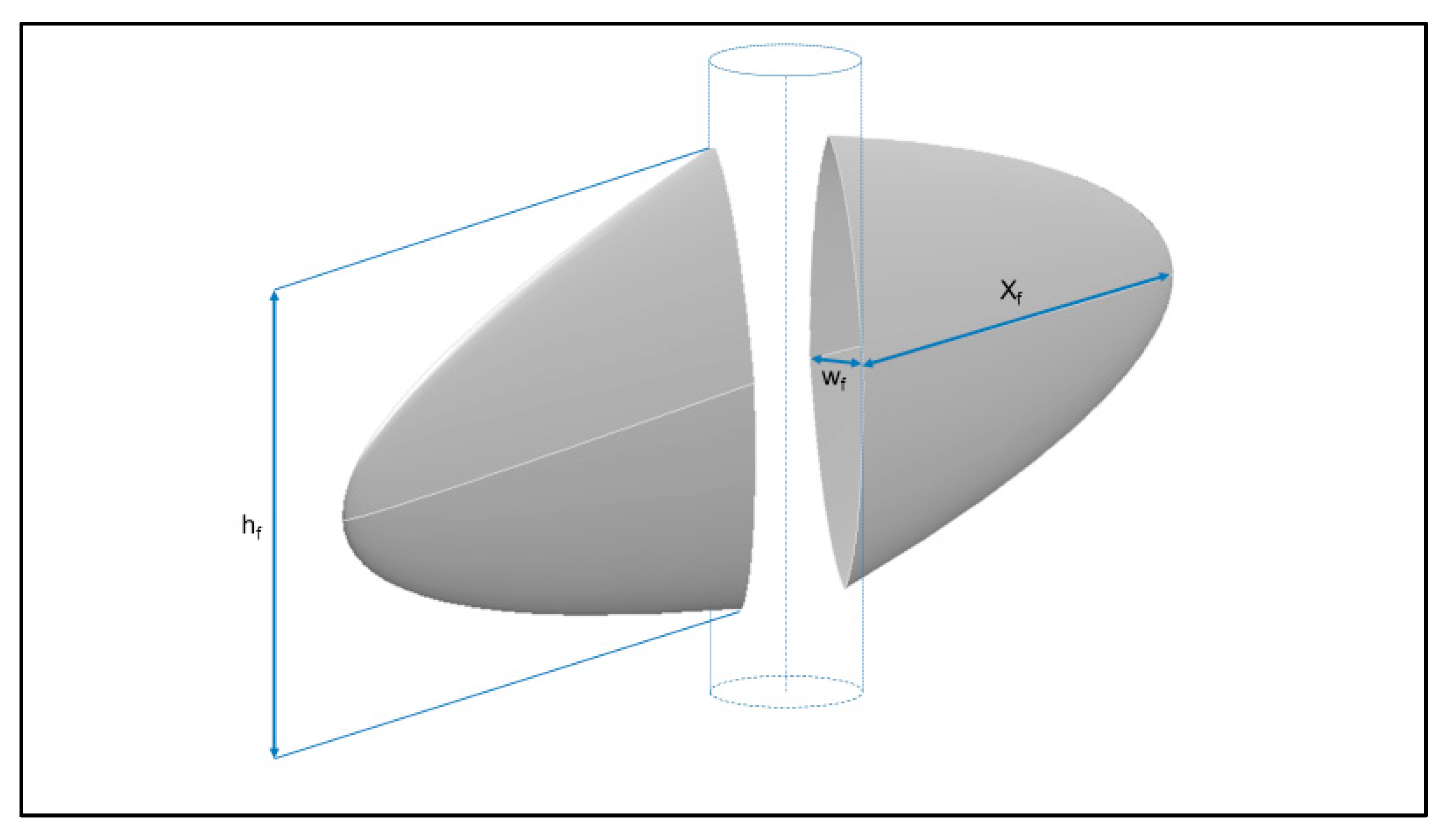
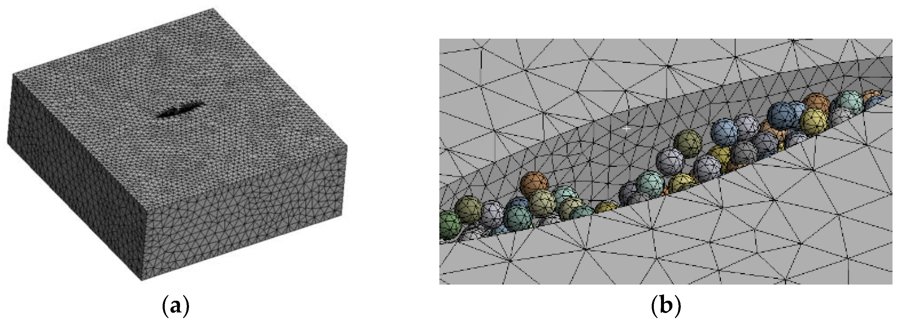
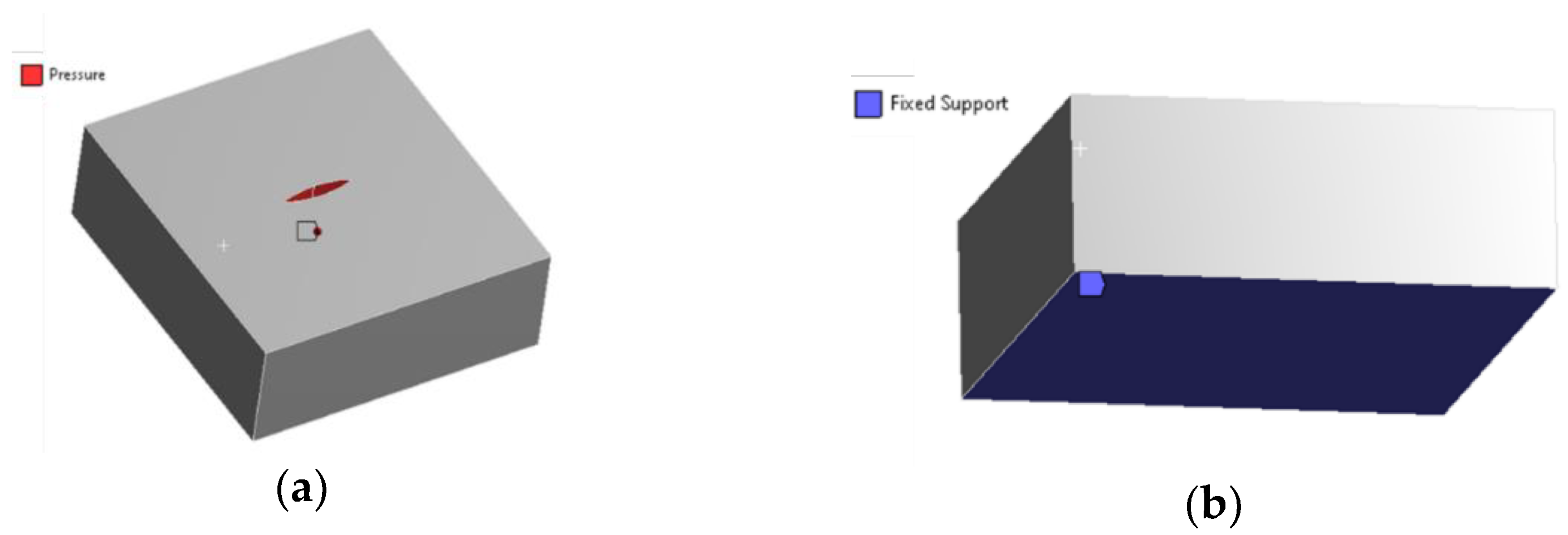
2.1.1. Geometry

During building up of the model concept, a conventional vertical well was considered to be fractured. In a vertical well, a classic bi-wind fracture formation takes place (assuming ideal in situ stress conditions) with the dimensions of fracture height, width, and half-length. In the 20th century, 2D models were developed and used for hydraulic fracture simulation. Basically, three models were used: radial, KGD, and PKN, where KGD and PKN are named after their inventors.

Various radial models were introduced, but all could be characterized by a fracture height directly related to fracture length and described by the radius. The KGD model, introduced by Zheltov and Khristianovic [26], used a fixed fracture height and a width proportional to the fracture length. Perkins and Kern [27] developed the PKN model, and it assumed a constant fracture height as well but a proportional fracture width to the fracture height. However, these models were used widespread, the desire for a more sophisticated solution made its way, and 3D models came into the picture. In our method, an elliptical fracture was created to consider the TSO (Tip Screenout) effect and represent flow patterns occurring in that case. Figure 1 demonstrates the schematic of the model geometry investigated in our research.

In reality, even with microseismic data available, simplifications are applied to model the hydraulic fracture. The main examined parameter, the fracture conductivity, is the product of permeability and fracture width, which allows one to investigate the phenomenon in a scaled-down but representative environment. According to the fluid dynamics, permeability does not depend on the spatial dimensions enabling us to reduce the fracture length and height, which may take more than 100 and 40 m in a well, respectively. Considering the complexity of the industrial problem and the calculation limit of both the software and computers (even supercomputers), a pragmatic approach was applied, and the fracture geometry was defined as presented in Figure 2 (dimensions in mm).

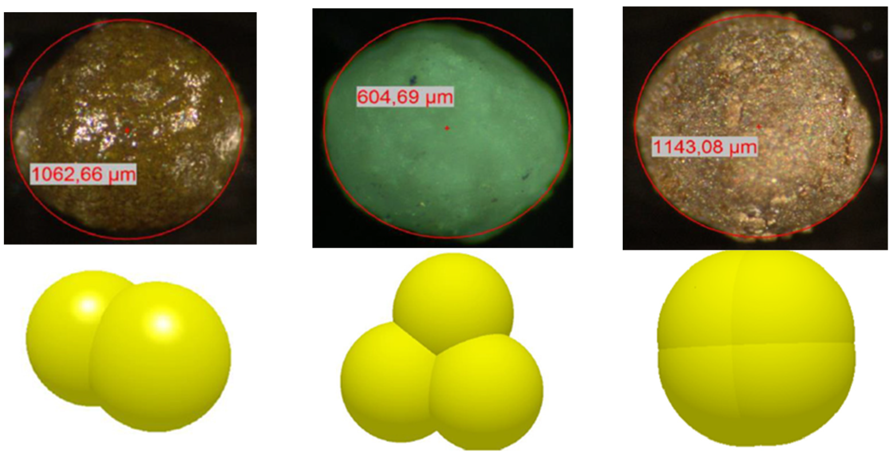
2.1.2. Reservoir and Proppant

As described in the introduction, the fracture conductivity is investigated after hydraulic fractures are created, propped, and the high-pressure hydraulic pumps placed at the surface are stopped, entailing the formation to close again. Boundary conditions were defined for the reservoir and the proppant itself to investigate the phenomenon relevantly.

The hydrocarbon-bearing reservoir characteristics directly impact the formation Young’s modulus and Poisson’s ratio, closure pressure, fluid pressure, and fluid flow. Therefore, the boundary condition for rock Young’s moduli was defined for a wide range providing an environment to investigate the effect of formation elasticity to proppant embedment and fracture conductivity in soft, well-consolidated, or even tough deposits, igneous or metamorphic rocks. The minimum value for formation Young’s moduli was defined as 1 GPa according to the research conducted by Lacy et al. [7], who examined proppant embedment and fracture conductivity in soft formations. Max and mean values were defined as 30 and 15 GPa referred to Malkowski and Ostrowski’s scientific work [29] in which more than 500 core samples have been measured to determine rock Young’s moduli. Since Poisson’s ratio of the reservoir does not have a significant influence on the examined phenomenon, it was fixed to 0.22, referring to the article published by Chan et al. [30]. The latter studied the depth of proppant embedment in hydraulic fractures.

For the relation of overburden, pore, and closure pressure the widely known Hubbert and Willis [31] formula was used:

σ_c = ν/(1 − ν) * (σ_v − αp_r) + αp_r,

(1)

where σ_c is closure stress / pressure [MPa], ν is Poisson’s ratio [-], σ_v is overburden or vertical stress [MPa], α is Biot’s poroelastic constant [-] and p_r is pore pressure [MPa]. One should note that this equation proposes that the in situ horizontal stress is generated by the uniaxial vertical strain without any tectonic activity. The pore pressure in the reservoir is supposed to be hydrostatic, while the overburden pressure was considered by the weight of the rocks assuming a medium sandstone density of 2.74 g/cm^3, according to Chaveste et al. [32]. They dealt with rock moduli and density determination using wireline data. Finally, the limits of closure pressure values used in our research were defined as 2139 and 13,904 psi that equals ~14.7 and 95.9 MPa in SI units, respectively. These closure pressure values also cover a wide range for investigating the effect of fracture pressure in shallow, medium, and even deep wells with a high amount of overburden.

Another relevant parameter to investigate the fracture behavior and fracture conductivity is the fluid flow in the fracture. In the case of hydraulic fracturing, several flow regimes are interpreted during the production period of the well. Cinco et al. [33] defined four flow patterns for hydraulically fractured wells: fracture linear flow, bilinear flow, formation linear flow, and pseudo-radial flow. Figure 3 represents the schematic of them. The conductivity we investigated is independent of the flow patterns and can be used for all the cases. According to the research published by Palish et al. [34], inertial flow is one of the parameters that can reduce the effective fracture permeability and conductivity significantly. The flow rate in our model was determined in a way that allows one to consider pressure drop due to not only Darcy but also non-Darcy effects, enabling one to conclude a real fractured well. Inertial forces occur during fluid flow at high velocities; therefore, conductivity was investigated at 0.144 kg/s mass flow, meaning a water flow rate of 78.4 BPD. Since permeability is independent of the medium (the Darcy equation and all the differential equations for fluid flow contain viscosity and density), water with 2% of KCl content was applied in the CFD model because its rheological parameters are well-known and do not restrict the applicability as in case of special light, heavy, sweet, or sour oil. The density and the viscosity of the water flowing through the propped fracture were 998 kg/m³ and 0.001003 Pas.

Proppant mechanical characteristics were defined after Chen et al. [30], who examined proppant with Young’s modulus of 41,306 MPa, Poisson’s ratio of 0.25, and proppant density of 2.8 g/cm³. Proppant geometry was considered to be spherical. Simulations were run for cases of the particle diameter of 1 mm, 1.37 mm, and 1.74 mm, which sizes represent the bigger available proppants on the industrial market, 16/20, 12/18, and 12 mesh, respectively [35].

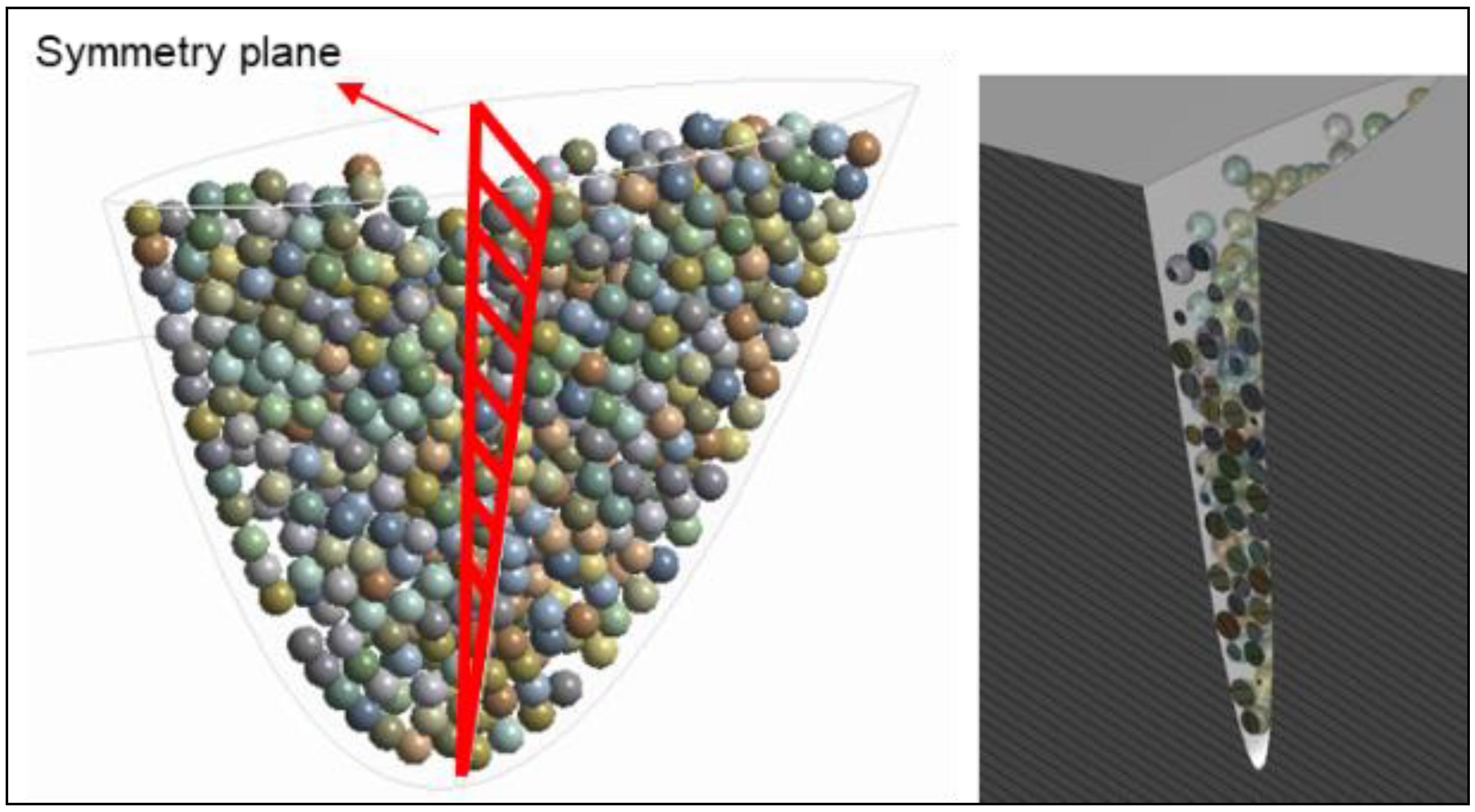
2.2. Discrete Element Modeling

The discrete element method (DEM) was used to fill the fracture with proppant particles. DEM is a relatively new numerical approximation method that can determine the characteristic displacements of particle systems. The peculiarity of the process is that it solves the governing equations of motion for each particle through a series of but finite time intervals. Interaction forces resulting from the collisions of the particles are evaluated by a contact model [36]. Research and practicing engineers have successfully applied it in many areas of engineering areas such as the pharmaceutical industry [37], agriculture [38], nuclear industry [39], etc.

For the numerical calculations, freeware software YADE [40] was used. The approximation method is based on the repeated solution (Figure 4) of Newton’s second law of motion and the general rotational equation according to all single elements implemented in the model. As an initial condition, we have to know the position of particles and external loads (e.g., gravity). Furthermore, during the solution, the particle–particle and particle–wall collisions have to be detected.

The contact model allows the interaction force system for every collision to be calculated, and, based on initial displacements of single elements, new positions can also be evaluated. Subsequently, it is necessary to upgrade the kinematic parameters of the whole system, and the simulation cycle has to be repeated. Thus, by the continuous solution of fundamental laws of dynamics, the granular assembly’s displacement, velocity, and acceleration field can be determined [36].

Generally, collisions are estimated by a spring-dashpot system. There are at least five different micromechanical parameters for each material in the simplest scenario and other model parameters (e.g., element shape, simulation time step, etc.).

Determining the micromechanical parameters of granular media makes numerical modeling very complicated and lengthy. In most cases, it takes more research and time to calibrate the parameters than to create and solve a discrete element model [42]. The primary reason for the problem is that the result of the modeling depends mainly on the mechanical constants of the interactions between the discrete elements, i.e., on the micromechanical parameters characteristic of the given assembly.

Due to the numerical approximation, in many cases, the experimentally determined value of some micromechanical parameters that direct measurements can determine does not lead to the most accurate results. Still, the behavior of the whole assembly can be described with sufficient accuracy, even with several combinations of parameters. It might be happening that there are multiple combinations of micromechanical parameters that result in the same macro behavior of the granular assembly; hence the calibration procedure must be very rigorous to get proper parameters. Owing to this, properties of individual particles may be determined by comparison of measured and numerical macro behavior of a particular physical process (calibration procedure) [43].

YADE uses perfectly rigid, so-called BALL type elements (Figure 5 shows the series of two springs representing normal stiffness of contact between two spheres) and generally normal (kN) and shear stiffness (kS) to describe interactions.

If the colliding elements having Young’s modulus E₁ and E₂ [MPa], radiuses r₁ and r₂ [mm], respectively, normal stiffness of colliding particles is

$$k_N=\frac{2E_1{r}_1{E}_2{r}_2}{E_1{r}_1+E_2{r}_2}$$

(2)

The value of shear stiffness can be calculated by a predefined ratio of normal stiffness value [38]. The displacement coordinates of individual elements (normal-u_N and shear displacement u_S) are calculated by geometrical parameters of interactions. The normal displacement u_N is

$$u_N=|C_2^{°}-C_1^{°}|=|C_2^{}-C_1^{}|$$

(3)

where C₁ and C₂ [-] denote reference centers of colliding elements when the interaction is established, while $C_1^{°}$ and $C_2^{°}$ correspond to centers of interacting particles as these can move during the simulation. Shear displacement u_S [mm] is calculated by adding the motion of the contact point in global space and the joint movement of colliding elements [40].

Normal and shear components of interaction forces are calculated by the contact model considered both of the displacements:

$$F_N=k_N{u}_N$$

(4)

$$F_S^{}=\{\begin{array}{cc}{F}_{N}tan\phi & \begin{array}{cc}if& \left|k_S{u}_S\right|>\end{array}{F}_{N}tan\phi ,\\ k_S{u}_S& \end{array}$$

(5)

where φ denotes friction angle [°] between colliding elements [40]. Ensuring numerical stability of discrete element simulations, there is a threshold limit of the simulation time step (Δt_cr) in YADE [39]:

$$\Delta t_{crit}=\frac{2}{{\omega }_{max}}=\underset{i}{min}\sqrt{2}\sqrt{\frac{m_i}{K_i}}$$

(6)

where ω_max [-] corresponds to the highest eigenfrequency within the model, m_i [kg] denotes the mass of the i-th particle, and K_i [N/mm] is the stiffness of the i-th spring. The unbalanced force is used for characterizing the numerical stability of models in YADE. This artificial force is calculated by the ratio of summarized forces on all bodies and mean forces acting on interactions. If the system is in perfectly static equilibrium, the summarized force on all bodies tends to zero, so thus unbalanced force will converge to zero in a quasi-static state [40].

Calibration Procedure

In our prior work [44], the shape and micromechanical parameters of proppant particles were determined. The sphericity of the proppant particles used in practice is nearly 90%; therefore, the particles were modeled as perfect spheres. Silo outflow was selected as a parameter identification technique. During the measurements, the mass of the discharged particles was recorded by three load transducers. In the case of granular media, the mass–time function always shows a linear nature. Due to this fact, linear regression was used to compare the measurements and numerical results. The average outflow mass flow rate (slope of the linear mass–time function) was used as the comparison parameter.

Using the parameters in

Table 1. Calibrated micromechanical parameters of proppant particles [40].

Parameter	Proppant	Silo
Poisson-ratio, ν [-]	0.25	0.3
Young modulus, E [Pa]	5 × 1010	-
Density, ρe [kg/m3]	5100	5100
Friction angle, φ [°]	10	1
Coeff. of rolling friction, f [m]	0.0001	0

, the computed and measured discharge rates showed sufficient fitting (Figure 6). In Figure 6 falling particles also can be seen colored by vertical velocity. This implies that the created particle model and the calibrated set of micro parameters can be utilized for DEM modeling of proppant particles.

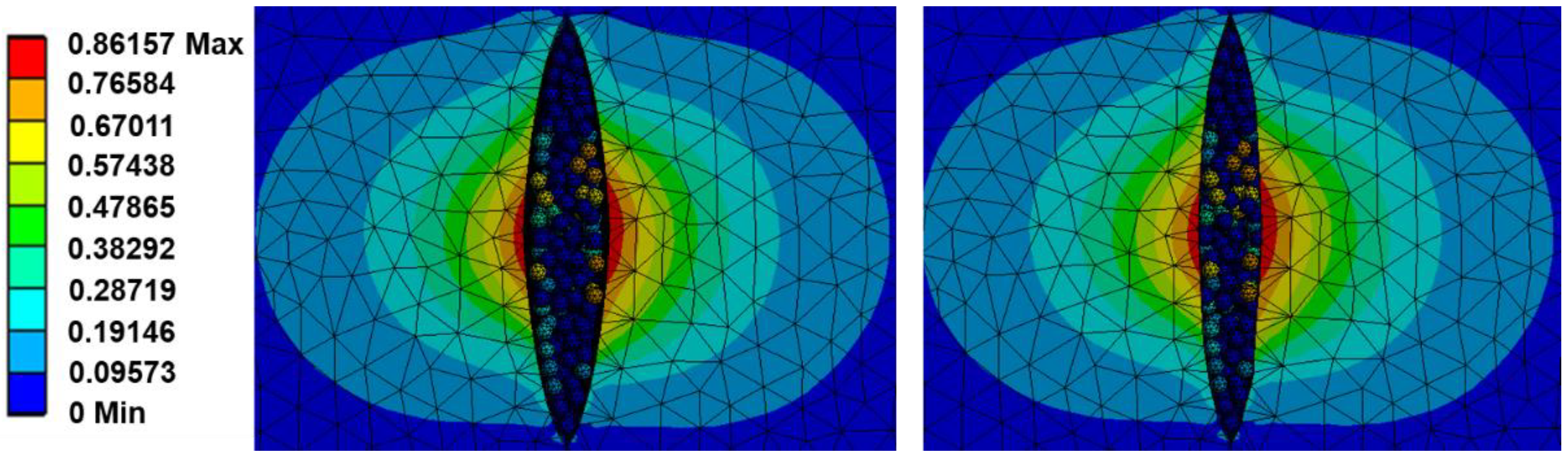
2.3. Finite Element Modeling

To determine the proppant pack’s deformation, finite element analysis was applied. The concept of this method was developed in the mid-1950s by Turner et al. [45] and has become an indispensable tool in engineering practice in recent decades.

Finite element modeling enables one to create a mathematical model that includes geometry, material models of the individual elements, boundary conditions, and contacts between the elements. The essence of the method is decomposing the investigated geometry into finite but tiny elements connected by nodes. At these nodes, the solution of the system of equations is searched that describes the relationship between input and output quantities. For instance, in stress analysis, the input quantity is the force from some load, and the output quantity is the displacement. Stiffness creates a connection between these quantities. During the preprocessing, one creates geometry, performs possible simplifications on the given geometry, then defines the material models of each part and the necessary contacts. The next step is to make the numerical mesh and then specify the loads and boundary conditions that describe reality in the most precise way. During the solution, the load vector (F) and the stiffness matrix (K) is produced, and the displacement (U) of the nodes is found by solving the prescribed system of equations:

K × U = F → U

(7)

Based on the force–displacement diagram of the given task, linear and nonlinear problems are distinguished. If the model contains contacts, a nonlinear problem is examined. In this case, Equation (7) is modified to the following form:

K(U) × U = F → U

(8)

By knowing the node displacements, secondary quantities, deformations, and stresses can be determined [44].

For numerical calculations of the deformation of the proppant particles, ANSYS 19.2 software was utilized.

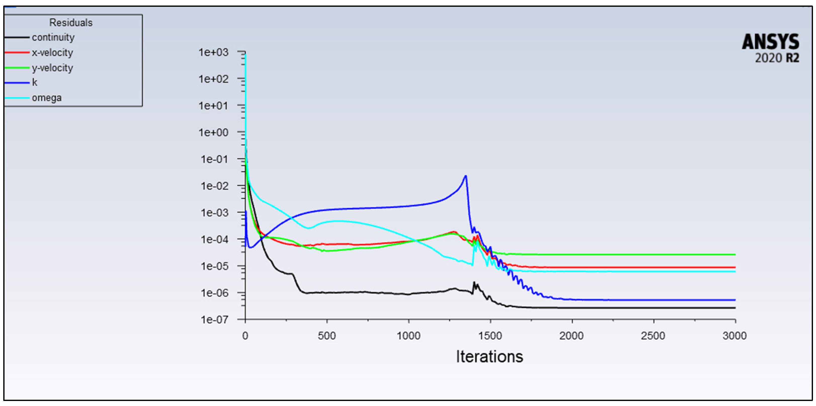
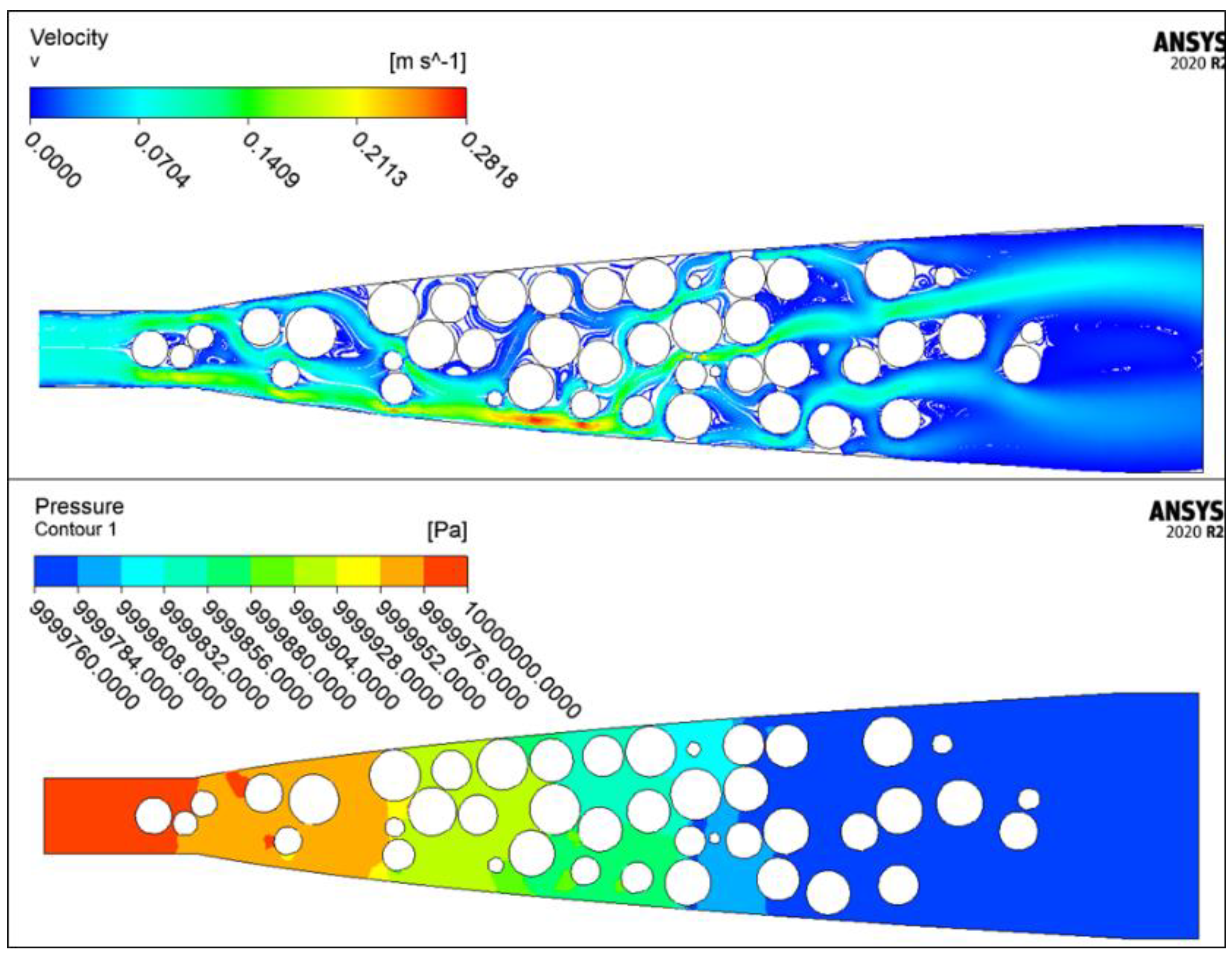
2.4. Computational Fluid Dynamics

After the fracture was filled and the deformation of proppant particles and formation was examined, fluid flow through the deformed propped fracture was investigated using computational fluid dynamics (CFD) software. In physics and engineering, fluid dynamics describes the flow of fluids—liquids and gases. According to John D. A. [46], three approaches exist in the history of fluid dynamics. The first approach is experimental fluid dynamics, which were laid in the 18th century in England and France. There was a gradual development of theoretical fluid dynamics in the 18th and 19th centuries, primarily in Europe. In the 1990s, the appearance of high-speed computers and the development of accurate numerical algorithms have revolutionized fluid dynamics. The third approach has been introduced as computational fluid dynamics. The CFD solvers are based on the fundamental governing equations of fluid dynamics. They use the continuity, momentum, and energy equations to describe the flow of fluids.

The essence of the continuity equations is that mass is neither created nor destroyed in the control volume. The control volume is a closed volume within the finite region of the flow. The integral form of the continuity equations can be written as:

$$\frac{\partial }{\partial t}{{\displaystyle \iiint }}_{\mathrm{V}}^{}\rho dV=-{{\displaystyle ∯}}_{\mathrm{S}}^{}\rho u·dS,$$

(9)

where ρ is the fluid density [kg/m³], u is the flow velocity [m/s] and t is time [s]. On the left side rate of change of mass can be found, while the term on the right side means the net inflow of mass.

The momentum equations are based on Newton’s second law of motion. The point is the equilibrium of the fluid’s rate of change of momentum to the external forces acting on the fluid within the control volume. The integral form of momentum equations:

$$\frac{\partial }{\partial t}{{\displaystyle \iiint }}_{\mathrm{V}}^{}\rho udV=-{{\displaystyle ∯}}_{\mathrm{S}}^{}\left(\rho u·dS\right)u-{{\displaystyle ∯}}_{\mathrm{S}}^{}p dS+{{\displaystyle \iiint }}_{\mathrm{V}}^{}\rho f_{body}dV+F_{surf}.$$

(10)

The term on the left side of the equation is the change of the momentum within the control volume, while on the right side, the terms represent the net inflow of momentum, total pressure, total viscous force, and total body force [46].

The third type of equation is the energy equations, which states that the energy can convert one form to another, and the total energy in a closed system remains constant. The energy equation can be written in the following form:

$$\rho \frac{De}{Dt}=-\nabla ·p-p\left(\nabla ·\mathrm{V}\right)+\dot{Q}$$

(11)

where e is the internal energy [J], p is the vector field of the heat flux by thermal conduction, and $\dot{Q}$ [J/s] is the rate of internal heat generation by the effects such as viscous friction or radiation [47].

For numerical calculations of the flows through the proppant particles, ANSYS CFX software was utilized.

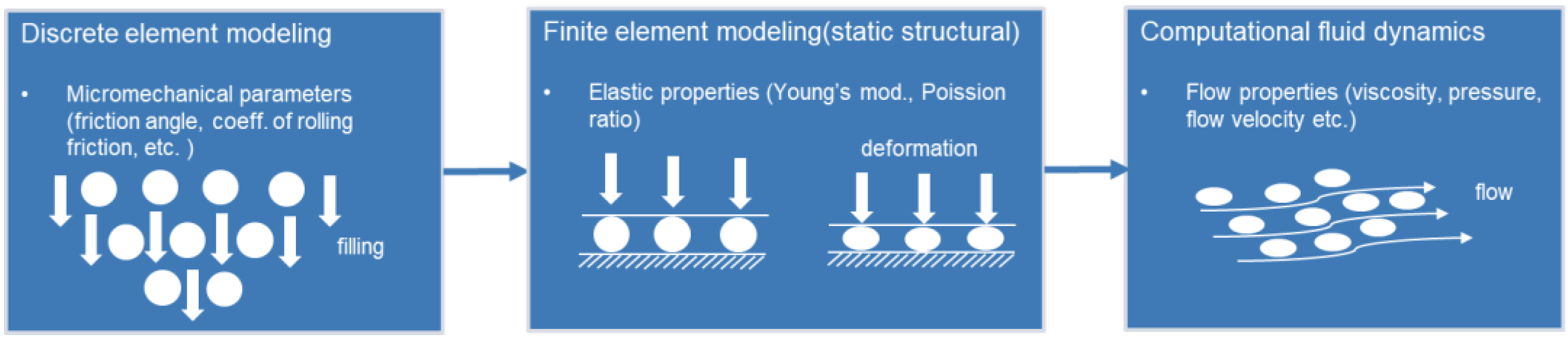
2.5. The One-Way Coupling Method

To describe the mechanical behavior of proppant particles one-way coupling method was developed. This method contains the results of DEM, FEM (structural analysis), and CFD. The particles generated and placed in DEM software were converted into FEM static structural module, where deformation of proppant and formation (embedment) due to the closure pressure was determined. Then the deformed assembly was converted into CFD environment where pressure drop due to the “resistance” of the propped fracture to the fluid flow could be calculated. The flow chart of the method can be seen in Figure 7.

3. Results

As introduced above, DEM simulation was used to generate fractures filled by the particles. The first step is generating the particles in the model space randomly. Although a regular layout is easy to create, this particle generation procedure can distort the behavior of the particle assembly [40]. Due to this reason, YADE software applies a random particle generation technique. At the beginning of the simulation, proppant particles were randomly generated in a closed box placed above the fracture. The box was closed until the summarized kinetic energy of elements decreased almost to zero (the system reached a quasi-static state). Then the bottom of the box was opened, and the particles could fell into the fracture under gravity. This random particle placement procedure allows the representation of proppant transport and placement by the fracturing fluid, neglecting particle settlement by gravity. The filled fracture can be seen in Figure 8.

The resulting geometry was pushed by an artificial assembly from the top of the fracture with 500 psi to enable proppant compaction and slippage, which occurs during actual fracturing and is considered in API standard proppant conductivity measurements [48], and then converted into FE software environment.

The first step in the FEA analysis was to specify the material properties. As described in Section 2.1.2, the proppant Young’s modulus and Poisson ratio were 41,306 MPa and 0.22. The Young’s modulus of the formation was systematically varied in a range of 1000 MPa to 30,000 MPa. The Poisson ratio was 0.22 in each case. The second step was to create a numerical mesh; then, the parts were meshed using second-order tetrahedron elements. Finally, mesh refinements were applied to the stress concentration areas, such as the particles and surfaces of the fracture. Mesh of the assembly can be seen in Figure 9, while

Table 2. Number of the nodes and elements.

Proppant Diameter [mm]	Nodes	Elements
1	379,043	187,117
1.37	195,523	100,071
1.74	173,006	93,518

summarizes the nodes and elements in each case.

One constraint was applied during the simulations to model fracture behavior: fixed support was used at the bottom of the formation (Figure 10b). In contrast, negative pressure was applied on the inside surfaces of the fracture to demonstrate the closure pressure acting as the initiator of deformation and embedment (Figure 10a).

Contact behavior was applied and modeled on connecting surfaces. There were only bonded contacts in the model, entailing no sliding or separation between faces or edges allowed. Automatic contact detection was utilized in the FEA software. The default contact formulation was adjusted Multi-Point Constraint (MPC) to bonded contacts. In Figure 11 undeformed and deformed assembly can be seen colored by the extent of total deformation. The deformed body is represented at two times magnification to get the results perceived. Comparing and analyzing the assemblies, one can obtain that the contacts worked well according to the rock and proppants’ visible displacement and deformation.

After FEM simulated deformation, static structural deformed geometry was exported into ANSYS CFX environment. To reduce the number of nodes and the computational time to achieve reasonable computational efficiency, the fracture was halved along a symmetry plane of the deformed assembly, assuming similar behavior for the rest of the fracture. Figure 12. shows the analyzed cross-section of the formation and proppants.

During the CFD analysis, the pressure drop was determined. To describe the fluid flow, one of the most commonly used turbulence models, the k-omega turbulence model, was applied. The cross-section was meshed using second-order tetrahedron elements, as in the case of FEM. Mesh refinement was applied to the areas between the particles to make the model more accurate. For better visibility, the cross-section was rotated 90 degrees. To define the boundary conditions well, the bottom and the top of the fracture were extended. The pore pressure for all runs was set to be 100 bar allowing one to make comparisons and draw conclusions, while the fluid mass flow was considered to be 0.144 kg/s as described in Section 2.1.2. Figure 13 shows the numerical mesh of the CFD model, while Figure 15 represents a typical case of velocity distribution within the fracture.

In the calculations, convergence was checked continuously. For evaluating convergence, the residuals plot can be used as the primary tool. The solver performs iterative solutions of the fundamental equation of CFD. Therefore, residuals should be as low as possible. In Figure 14, the residuals of one of the simulations can be seen. In each case, the lowest value of the residuals was under 10⁻⁴, which is the default criterion value in most of the CFD software. In Figure 15, one can see the velocity and pressure distribution between the particles.

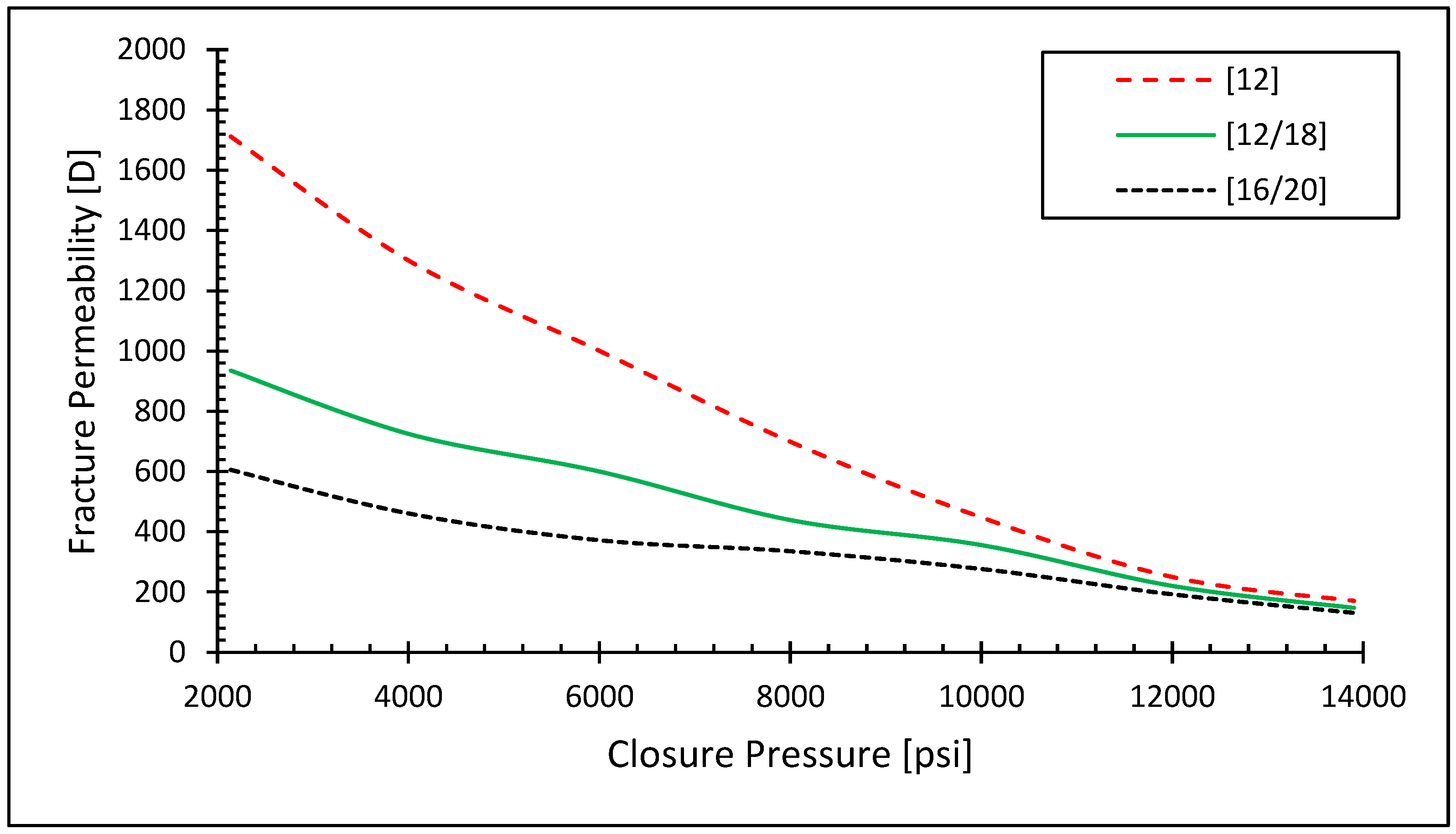
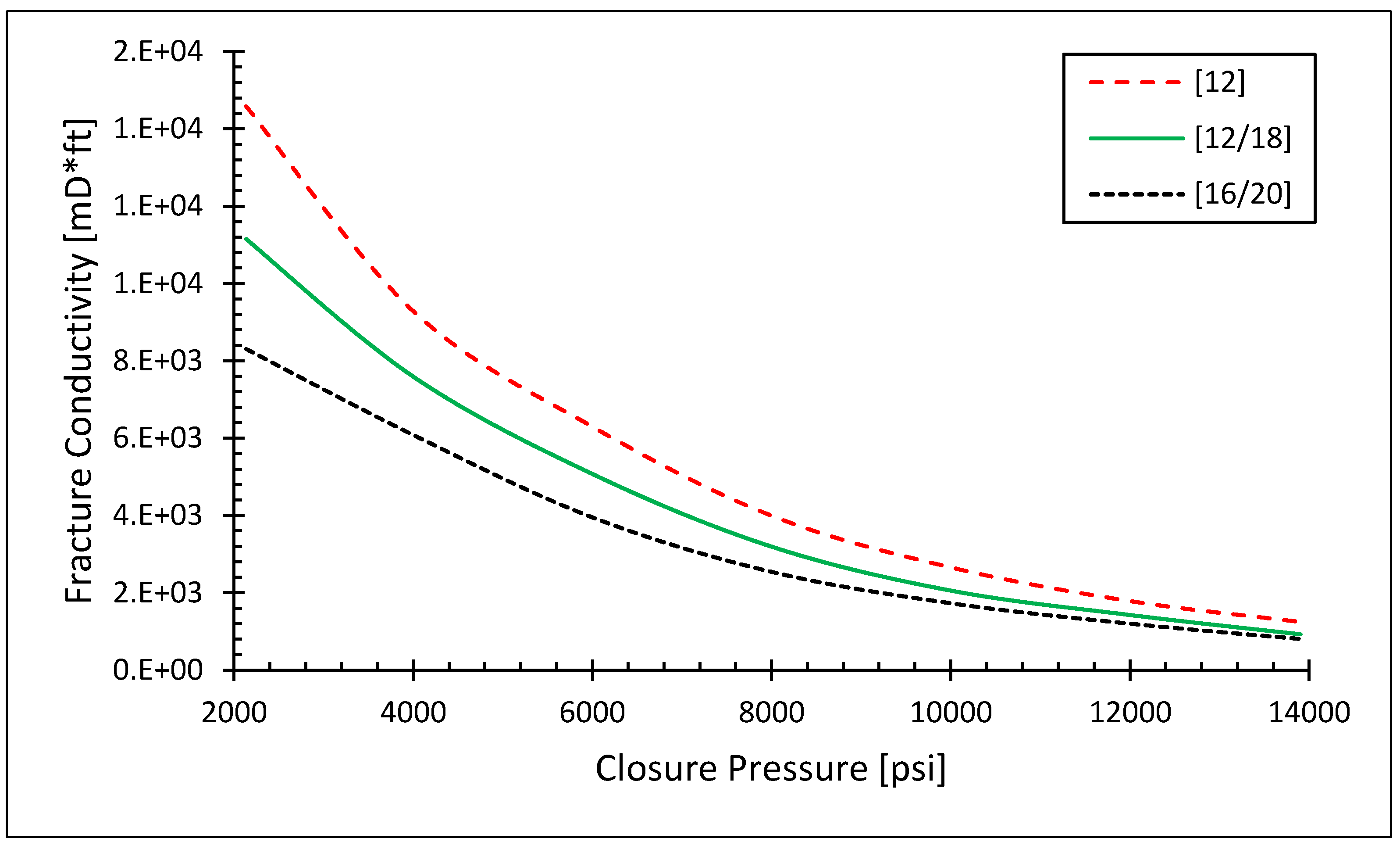
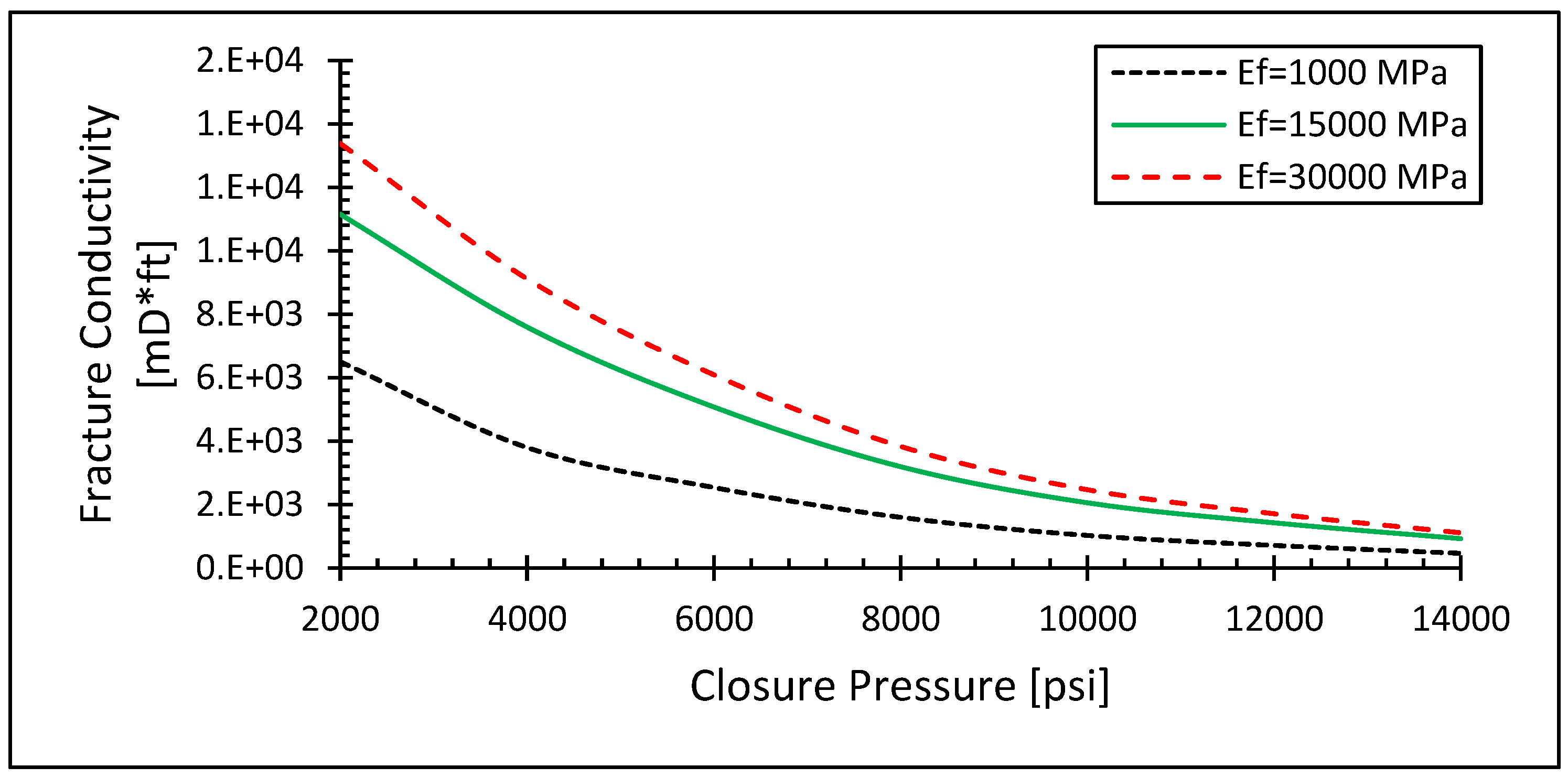
Sensitivity Analysis

By application of the fore-mentioned one-way coupling method, a parameter sensitivity study was performed to analyze behaviors of proppant particles for a pressure drop of the medium flowing between particles. As previous research showed, the main parameters that affect propped fracture behavior concerning permeability and conductivity are the closure pressure, Young’s modulus of the formation, and proppant diameter. Therefore, the effect of these factors was investigated in a predetermined relevant range according to chapter Section 2.1.2:

• Closure pressure (P_c) 2139–13,904 psi;
• Young’s modulus of the formation (E_f) 1–30 GPa;
• Proppant diameter (D_p) 1–1.74 mm.

In the first part of the sensitivity study, the effect of closure pressure was investigated. The Young’s modulus of the proppant particles was 41,306 MPa, while the Young’s modulus of the formation was 15,000 MPa. The diameter of proppants was 12, 12/18, and 16/20 mesh, as described in Section 2.1.2. The closure pressure was ranged from 2139 to 13,904 psi by 2000 psi steps, and the corresponding pressure drops were recorded at each simulation. Defining a mean value for the cross-section where the fluid flows through and using Darcy’s law, apparent permeability could be calculated. Figure 16 and Figure 17 demonstrate permeability and conductivity results as a function of closure pressure.

As expected, proppant pack permeability or other defined the permeability of the propped fracture decreases as closure pressure increases. Again, this phenomenon is anticipated since the formation pressure generates load on the propped fracture entailing a closing action which deforms and embeds proppants into the formation reducing the size of pore throats where fluid could flow.

Another critical point is the impact of proppant particles on fracture permeability. The diameter of the proppant has a remarkable influence on fluid dynamics. As Petrophysics predicts exponentially higher permeability value for rocks formed by greater particles of sediment, crystalline or metamorphic components, the same, or even more significant effect—because no cementation considered this case―could be observed in case of propped fractures. Analyzing the sensitivity test results in Figure 16 one can also conclude that the greater the proppant size, the more permeability reduction takes place. By approximating the closure pressure value of 12,000 psi, different proppant diameters produce similar permeability. This phenomenon can be explained as follow: a proppant pack formed by greater particles can deform to a greater extent because more pore space is available to be reduced. Consequently, pore space is getting smaller with closure pressure, and permeability approximates the case of proppant packs formed by particles with lower diameters.

Comparing our one-way coupled model results and laboratory test results published by Fan et al. [21], one can identify permeability values with the same magnitude, i.e., our DEM–FEM–CFD model resulted in 935 D (Figure 16, 12/18 mesh). In contrast, lab test ~ 2700 D. The difference could be traced back to reasons summarized by Palish et al. [34] about API RP-61 conductivity testing standard versus realistic fracture conductivity, which implies additional permeability reduction due to inertial forces not representing by flow regimes (2 mL/min) applied at conductivity testing standards. Another indicator of the difference could be the ideal―evenly distributed―proppant placement and “fracture” geometry demonstrated by the conductivity cell in API standards as an artificial, manufactured assembly.

The known conditions for Figure 17 were taken to be the same as Figure 16: Young’s modulus of proppant particles was set to be 41,306 MPa, while Young’s modulus of the formation was 15,000 MPa, the diameter of proppants was ranged from 12 mesh to 16/20 mesh. Fracture conductivity is directly dependent―calculated as the product of fracture width and proppant pack permeability―on fracture permeability, Figure 17 illustrates similar curves as Figure 16 did, i.e., closure pressure has a relevant impact on fracture conductivity. Since both fracture width and permeability are affected by the formation’s closing action, the impact of closure pressure on fracture conductivity can be interpreted as the superposition of fracture width and permeability reduction. Therefore, fracture conductivity could be decreased to one-sixth at 10,000 psi in the case of 12 mesh, while this reduction is only one-fourth for permeability.

Proppant size has a more relevant impact on fracture conductivity than permeability. It can be explained by the definition of conductivity as well. The bigger the proppant, the greater the negative effect of closure pressure on fracture width and permeability as described above, i.e., the conductivity difference for different proppant sizes reduces at a higher rate with closure pressure.

Figure 18 was performed to investigate the effect of closure pressure on fracture conductivity for different Young’s modulus of the hydrocarbon-bearing formation. The known conditions were taken to be D_p = 12/18 mesh (proppant diameter), E_p = 41,306 MPa (proppant Young’s modulus), and E_f—denoting Young’s modulus of formation―was set to be 1000, 15,000, and 30,000 MPa. The tendency is similar to the diagrams presented previously. However, a complete evaluation gives exciting results. Since the elastic modulus of formation is directly proportional to proppant embedment and nothing else, one can conclude that embedment in the case of soft formation, e.g., shale, can affect fracture conductivity in a large-scale way. Nevertheless, the difference between conductivity values for different Young’s modulus gets smaller with closure pressure, as noticed in the previous sensitivity analyses.

4. Discussion

Hydraulic fracturing treatment is used to enhance well productivity, usually drilled in tight or less permeable reservoirs by forming high-conductive channels between the formation and the wellbore. The closure pressure after fracturing indicates a closing action that is prevented by proppant particles placed between the fracture walls and which are bearing a complex stress condition. Even if proppants are enormously strong and the strength of the hydrocarbon-bearing layer is quite high, proppant deformation and embedment take place and may result in a significant reduction of the created fracture conductivity, particularly under high closure pressure circumstances. In this paper, a brand-new method was developed to model in-situ fracture behavior by coupling DEM–FEM–CFD numerical solutions. DEM was applied to generate and randomly place proppants into the fracture; meanwhile, FEM Static Structural module was used to let the proppants be deformed and embedded into the formation, and finally, Computational Fluid Dynamics application was coupled to investigate the permeability and conductivity of the propped fractures. To the best of our knowledge, this research marks the workflow of coupling DEM–FEM–CFD for propped fracture behavior modeling the first time.

This research showed that achievable fracture conductivity increases with the increase of proppant size and formation stiffness; however, it decreases with the increment of fracture-aperture-closing stress. Of course, these trends fit the results published by many researchers before, but the absolute value of the simulation results pointed out new perspectives of fracture behavior modeling. As many real factors―such as fracture geometry, uneven proppant and so stress distribution, proppant deformation and embedment, and industrial flow rate―have been integrated in our model, lower conductivity values could be observed, which fact allows one to consider this developed workflow as a more sophisticated approximation of the real phenomenon. Meanwhile, these results also confirm the conclusions drawn by Palish et al. [34], i.e., proppant conductivity measuring standards may result in overestimated conductivity values compared to achievable ones in the underground.

This current work also highlighted some future perspectives in the direction of how to describe the phenomenon more precisely. Following the way of our previous work, the implementation of non-perfect spheres as proppants may make another breakthrough. Figure 19 represents our electron microscopic examination of proppants and DEM clumps approximating proppant particle geometry which is usually characterized by sphericity and roundness indices. Another potential is to consider proppant size distribution and generate proppants with different diameters according to their mesh size and sieve analysis that may result in further conductivity reduction.

This paper demonstrated the capability of DEM–FEM–CFD coupling for modeling multidisciplinary processes regarding hydraulic fracturing and provided insight into the factors that drive the comprehensive interactions between proppant particles, formation stiffness, and closure pressure. The outcome of this research may advance the fundamental understanding of proppant embedment and deformation and contribute to a broad scale of applied sciences that aim to optimize hydraulic fracturing.

References

1. Denney, D. Thirty Years of Gas-Shale Fracturing: What Have We Learned? J. Pet. Technol. 2010, 62, 88–90. [Google Scholar] [CrossRef]
2. Economides, M.; Nolte, K. Reservoir Stimulation, 3rd ed.; John Wiley and Sons: Hoboken, NJ, USA, 2000. [Google Scholar]
3. Barree, R.; Conway, M. Experimental and Numerical Modeling of Convective Proppant Transport (includes associated papers 31036 and 31068). J. Pet. Technol. 1995, 47, 216–222. [Google Scholar] [CrossRef]
4. Liang, F.; Sayed, M.; Al-Muntasheri, G.; Chang, F.F. Overview of Existing Proppant Technologies and Challenges. Presented at the SPE Middle East Oil and Gas Show and Conference, Manama, Bahrain, 15–18 March 2009. [Google Scholar] [CrossRef]
5. Huitt, J.L.; Mcglothlin, B.B. The Propping of Fractures in Formations Susceptible to Propping-sand Embedment. Presented at the Drilling and Production Practice, New York, NY, USA, 1 January 1958. SPE-58-115-MS. [Google Scholar]
6. Volk, L.J.; Raible, C.J.; Carroll, H.B.; Spears, J.S. Embedment of High Strength Proppant into Low-Permeability Reservoir Rock. Presented at the SPE/DOE Low Permeability Gas Reservoirs Symposium, Denver, CO, USA, 27–29 May 1981. [Google Scholar] [CrossRef]
7. Lacy, L.L.; Rickards, A.R.; Ali, S.A. Embedment and Fracture Conductivity in Soft Formations Associated with HEC, Borate and Water-Based Fracture Designs. Presented at the SPE Annual Technical Conference and Exhibition, San Antonio, TX, USA, 5–8 October 1997. [Google Scholar] [CrossRef]
8. Lacy, L.L.; Rickards, A.R.; Bilden, D. Fracture Width and Embedment Testing in Soft Reservoir Sandstone. SPE Drill. Complet. 1998, 13, 25–29. [Google Scholar] [CrossRef]
9. Guo, J.; Liu, Y. Modeling of Proppant Embedment: Elastic Deformation and Creep Deformation. Presented at the SPE International Production and Operations Conference & Exhibition, Doha, Qatar, 14–16 May 2012. [Google Scholar] [CrossRef]
10. Lehman, L.V.; Parker, M.A.; Blauch, M.E.; Haynes, R.; Blackmon, A. Proppant Conductivity—What Counts and Why. Presented at the SPE Mid-Continent Operations Symposium, Oklahoma City, OK, USA, 28–31 March 1999. [Google Scholar] [CrossRef]
11. Fredd, C.; McConnell, S.; Boney, C.; England, K. Experimental Study of Hydraulic Fracture Conductivity Demonstrates the Benefits of Using Proppants. Presented at the SPE Rocky Mountain Regional/Low-Permeability Reservoirs Symposium and Exhibition, Denver, CO, USA, 12–15 March 2000. [Google Scholar] [CrossRef]
12. Barree, R.; Cox, S.; Barree, V.; Conway, M. Realistic Assessment of Proppant Pack Conductivity for Material Selection. Presented at the SPE Annual Technical Conference and Exhibition, Denver, CO, USA, 5–8 October 2003. [Google Scholar] [CrossRef]
13. Weaver, J.D.; Rickman, R.D.; Luo, H. Fracture-Conductivity Loss Due to Geochemical Interactions between Manmade Proppants and Formations. Presented at the SPE Eastern Regional/AAPG Eastern Section Joint Meeting, Pittsburgh, PA, USA, 11–15 October 2008. [Google Scholar] [CrossRef]
14. McDaniel, G.A.; Abbott, J.; Mueller, F.A.; Mokhtar, A.; Pavlova, S.; Nevvonen, O.; Parias, T.; Alary, J.A. Changing the Shape of Fracturing: New Proppant Improves Fracture Conductivity. Presented at the SPE Eastern Regional/AAPG Eastern Section Joint Meeting, Pittsburgh, PA, USA, 11–15 October 2008. [Google Scholar] [CrossRef]
15. Cooke, C.J. Conductivity of Fracture Proppants in Multiple Layers. J. Pet. Technol. 1973, 25, 1101–1107. [Google Scholar] [CrossRef]
16. Roodhart, L.; Kulper, T.; Davies, D.R.K. Proppant-Pack and Formation Impairment during Gas-Well Hydraulic Fracturing. SPE Prod. Eng. 1988, 3, 438–444. [Google Scholar] [CrossRef]
17. Peard, N.; Macaluso, M.; Griffin, M.; Andress, R.; Callanan, M. Improved Fracturing Techniques Increase Productivity in the AWP (Olmos) Field. Presented at the SPE Production Operations Symposium, Oklahoma City, OK, USA, 7–9 April 1991. [Google Scholar] [CrossRef]
18. Milton-Tayler, D.; Stephenson, C.; Asgian, M. Factors Affecting the Stability of Proppant in Propped Fractures: Results of a Laboratory Study. Presented at the SPE Annual Technical Conference and Exhibition, Washington, DC, USA, 4–7 October 1992. [Google Scholar] [CrossRef]
19. Li, K.; Gao, Y.; Lyu, Y.; Wang, M. New Mathematical Models for Calculating Proppant Embedment and Fracture Conductivity. SPE J. 2015, 20, 496–507. [Google Scholar] [CrossRef]
20. Sun, J.; Hu, K.; Wong, J.; Hall, B.; Schechter, D. Investigating the Effect of Improved Fracture Conductivity on Production Performance of Hydraulic Fractured Wells through Field Case Studies and Numerical Simulations. Presented at the SPE Hydrocarbon Economics and Evaluation Symposium, Houston, TX, USA, 19–20 May 2014. [Google Scholar] [CrossRef]
21. Fan, M.; Han, Y.; McClure, J.; Chen, C. Hydraulic Fracture Conductivity as a Function of Proppant Concentration under Various Effective Stresses: From Partial Monolayer to Multilayer Proppants. Presented at the SPE/AAPG/SEG Unconventional Resources Technology Conference, Austin, TX, USA, 24–26 July 2017. [Google Scholar] [CrossRef]
22. Zhang, F.; Zhu, H.; Zhou, H.; Guo, J.; Huang, B. Discrete-Element-Method/Computational-Fluid-Dynamics Coupling Simulation of Proppant Embedment and Fracture Conductivity After Hydraulic Fracturing. SPE J. 2017, 22, 632–644. [Google Scholar] [CrossRef]
23. Fan, M.; McClure, J.; Han, Y.; Ripepi, N.; Westman, E.; Gu, M.; Chen, C. Using an Experiment/Simulation-Integrated Approach to Investigate Fracture-Conductivity Evolution and Non-Darcy Flow in a Proppant-Supported Hydraulic Fracture. SPE J. 2019, 24, 1912–1928. [Google Scholar] [CrossRef]
24. Zhu, H.; Shen, J.; Zhang, F. A fracture conductivity model for channel fracturing and its implementation with Discrete Element Method. J. Pet. Sci. Eng. 2018, 172, 149–161. [Google Scholar] [CrossRef] [Green Version]
25. Zhang, F.; Dontsov, E. Modeling hydraulic fracture propagation and proppant transport in a two-layer formation with stress drop. Eng. Fract. Mech. 2018, 199, 705–720. [Google Scholar] [CrossRef]
26. Zheltov, A.K. Formation of Vertical Fractures by Means of Highly Viscous Liquid. In Proceedings of the 4th World Petroleum Congress, Rome, Italy, 3 June 1955. [Google Scholar]
27. Perkins, T.K.; Kern, L.R. Widths of Hydraulic Fractures. J. Pet. Technol. 1961, 13, 937–949. [Google Scholar] [CrossRef]
28. Economides, M.J.; Tony, M. Modern Fracturing: Enhancing Natural Gas Production; ET Publishing: Houston, TX, USA, 2007; p. 96. [Google Scholar]
29. Malkowski, P.; Ostrowski, L. The Methodology for the Young Modulus Derivation for Rocks and Its Value. In Proceedings of the ISRM European Rock Mechanics Symposium-EUROCK 2017, Ostrava, Czech Republic, 20–22 June 2017. [Google Scholar]
30. Chen, M.; Zhang, S.; Liu, M.; Ma, X.; Zou, Y.; Zhou, T.; Li, N.; Li, S. Calculation method of proppant embedment depth in hydraulic fracturing. Pet. Explor. Dev. 2018, 45, 159–166. [Google Scholar] [CrossRef]
31. Hubbert, M.K.; Willis, D.G. Mechanics of Hydraulic Fracturing. Trans. AIME 1957, 210, 153–168. [Google Scholar] [CrossRef]
32. Alvaro, C.; Jimenez, J.R. Estimation of Moduli and Densities of Rock Constituents through Global Inversion of Wire-line Data. In Proceedings of the 2003 SEG Annual Meeting, Dallas, TX, USA, October 2003. [Google Scholar] [CrossRef]
33. Cinco-Ley, H.; Samaniego-V., F.; Dominguez, N. Transient Pressure Behavior for a Well with a Finite-Conductivity Vertical Fracture. Soc. Pet. Eng. J. 1978, 18, 253–264. [Google Scholar] [CrossRef] [Green Version]
34. Palisch, T.T.; Duenckel, R.J.; Bazan, L.W.; Heidt, J.H.; Turk, G.A. Determining Realistic Fracture Conductivity and Understanding its Impact on Well Performance-Theory and Field Examples. In Proceedings of the SPE Hydraulic Fracturing Technology Conference, College Station, TX, USA, 29–31 January 2007. [Google Scholar] [CrossRef]
35. Liang, F.; Sayed, M.; Al-Muntasheri, G.A.; Chang, F.F.; Li, L. A comprehensive review on proppant technologies. Petroleum 2015, 2, 26–39. [Google Scholar] [CrossRef] [Green Version]
36. Cundall, P.A.; Strack, O.D.L. A discrete numerical model for granular assemblies. Geotechnique 1979, 29, 47–65. [Google Scholar] [CrossRef]
37. Ketterhagen, W.R.; Curtis, J.S.; Wassgren, C.R.; Kong, A.; Narayan, P.J.; Hancock, B.C. Granular segregation in discharging cylindrical hoppers: A discrete element and experimental study. Chem. Eng. Sci. 2007, 62, 6423–6439. [Google Scholar] [CrossRef]
38. Oldal, I.; Keppler, I.; Csizmadia, B.; Fenyvesi, L. Outflow properties of silos: The effect of arching. Adv. Powder Technology. 2012, 23, 290–297. [Google Scholar] [CrossRef]
39. Keppler, I. Failure analysis of pebble bed reactors during earthquake by discrete element method. Nucl. Eng. Des. 2013, 258, 102–106. [Google Scholar] [CrossRef]
40. Šmilauer, V.; Chareyre, B. Yade dem formulation. In Yade Documentation, 1st ed.; Šmilauer, V., Ed.; The Yade Project: Lowestoft, UK, 2010. [Google Scholar]
41. Park, J.; Kang, N. Applications of fiber models based on discrete element method to string vibration. J. Mech. Sci. Technol. 2009, 23, 372–380. [Google Scholar] [CrossRef]
42. Bagi, K. Fundaments of the Discrete Element Method, 1st ed.; Budapest University of Technology and Economics: Hungary, Budapest, 2012; p. 73. [Google Scholar]
43. Keppler, I.; Safranyik, F.; Oldal, I. Shear test as calibration experiment for DEM simulations: A sensitivity study. Eng. Comput. 2016, 33. [Google Scholar] [CrossRef]
44. Varga, A.; Lengyel, T.; Safranyik, F. Determination of micromechanical parameters of proppant particles. IJIRAE Int. J. Res. Adv. Eng. 2020, VII, 15–21. [Google Scholar]
45. Turner, M.J.; Clough, R.W.; Martin, H.C.; Topp, L.J. Stiffness and Deflection Analysis of Complex Structures. J. Aeronaut. Sci. 1956, 23, 805–823. [Google Scholar] [CrossRef]
46. John, D.A. Computational Fluid Dynamics, the Basics with Applications International Editions, 1st ed.; McGraw-Hill Inc.: New York, NY, USA, 1995; pp. 60–75. [Google Scholar]
47. Bathe, K.J.; Saunders, H. Finite Element Procedures in Engineering Analysis. J. Press. Vessel. Technol. 1984, 106, 421–422. [Google Scholar] [CrossRef]
48. Renkes, I.; Anschutz, D.; Sutter, K.; Rickards, A. Long Term Conductivity vs. Point Specific Conductivity. In Proceedings of the SPE Hydraulic Fracturing Technology Conference and Exhibition, The Woodlands, TX, USA, 24–26 January 2017. [Google Scholar] [CrossRef]
Figure 1. Elliptical bi-wind fractures in a vertical well [28] (p. 96).
Applsci 11 09681 g001
Figure 2. Model geometry.
Applsci 11 09681 g002
Figure 3. Flow regimes after Cinco et al. [28] (p. 287).
Applsci 11 09681 g003
Figure 4. Simulation cycle of the Discrete Element Method [41].
Applsci 11 09681 g004
Figure 5. BALL type model in YADE.
Applsci 11 09681 g005
Figure 6. Comparison of measured and calculated mass–time functions [44].
Applsci 11 09681 g006
Figure 7. The flow chart of the method.
Applsci 11 09681 g007
Figure 8. Fracture filled by proppant.
Applsci 11 09681 g008
Figure 9. Numerical mesh of the formation (a) and proppant particles (b).
Applsci 11 09681 g009
Figure 10. Surface pressure inside the fracture (a) and fixed support at the bottom of the formation (b).
Applsci 11 09681 g010
Figure 11. The undeformed and deformed assembly (2× deformation).
Applsci 11 09681 g011
Figure 12. The analyzed cross-section.
Applsci 11 09681 g012
Figure 13. Numerical mesh of CFD analysis.
Applsci 11 09681 g013
Figure 14. Residuals of CFD analysis.
Applsci 11 09681 g014
Figure 15. Velocity and pressure distribution within the fracture.
Applsci 11 09681 g015
Figure 16. Fracture permeability as a function of closure pressure.
Applsci 11 09681 g016
Figure 17. Fracture conductivity as a function of closure pressure.
Applsci 11 09681 g017
Figure 18. Fracture conductivity for different formation Young’s modulus.
Applsci 11 09681 g018
Figure 19. Electron microscopic photos and DEM clumps.
Applsci 11 09681 g019