Acoustic Impact of Hybrid-Electric DEP Aircraft Configuration at Airport Level

Abstract

The Italian research project PROSIB (PROpulsione e Sistemi IBridi per velivoli ad ala fissa e rotante), is a 30-month initiative funded by the Italian Ministry of University and Scientific Research (MIUR) and coordinated by the Leonardo company. The project is aimed to investigate configurations for regional aircraft and rotary wing platforms and architectures for propulsion systems, and is dedicated to the identification of the best strategy for their use, given different on-board energy sources. The reduced environmental impact is the key for the success of the new hybrid/electric aircraft configurations. This not only considers the chemical pollution introduced in the atmosphere, but also the noise produced on the surrounding area of airports. The present paper describes the acoustic impact assessment resulting from the inclusion of new propulsion technologies and new configurations of regional aircraft (ATR42 pax) in a reference airport area.

1. Introduction

The Italian research project PROSIB (PROpulsione e Sistemi IBridi per velivoli ad ala fissa e rotante) [1], is a national project whose scope is the exploration of the impact of innovative propulsion technologies on regional aircraft and rotary wing platforms.

The future of aircraft propulsion is leadning to electric configurations, not only using fully electric technology, but also considering hybrid electric approaches. Engineering solutions will have the goal of finding the best strategies for optimizing all available energy sources on the aircraft, both electrical and classical. Electric propulsion systems are characterised by zero emissions, but we need to also take into account the noise levels produced by the system as a whole. The noise emitted by these propulsion systems is expected to be different from classical general aviation aircraft noise, particularly relevant to populated areas around the airports.

The present work is focused on the evaluation of the acoustic impact resulting from a regional aircraft (ATR42 pax) equipped with new propulsion technologies and new configurations.

Though noise impacts on the ground are usually evaluated with experimental test campaigns [2], this is not feasible when exploring a novel configuration. We propose a computational chain to assess the acoustic performances of aircraft in the preliminary phases of design. As a first step, to evaluate the real gain in terms of noise reduction it is important to characterize the aircraft as a noise source and then assess the impacts of its operation. Its noise field can be computed using the results of aerodynamic performance simulations. Then, a database of aircraft operations, in terms of noise levels, can be produced using the Noise–power–distance (NPD) approach [3].

Noise–power–distance (NPD) databases play a central role in conducting noise impact assessments for any type of aircraft. This is even more important when considering new configurations, such as those equipped with brand new hybrid/electric engines. As reported in [4], the Federal Aviation Administration, Office of Environment and Energy (FAA-AEE) developed an Aviation Environmental Design Tool AEDT that uses NPD results as a source term in evaluating aircraft noise and emissions for airport environmental studies.

Following the procedure described above, CIRA setup a computational chain consisting of the following main steps:

• The evaluation of the aerodynamic pressures on the full configuration via a medium-fidelity aerodynamic solver;
• The evaluation of aeroacoustic performances and hemispheric noise fields, using the Ffowcs Williams and Hawkings (FW–H) approach;
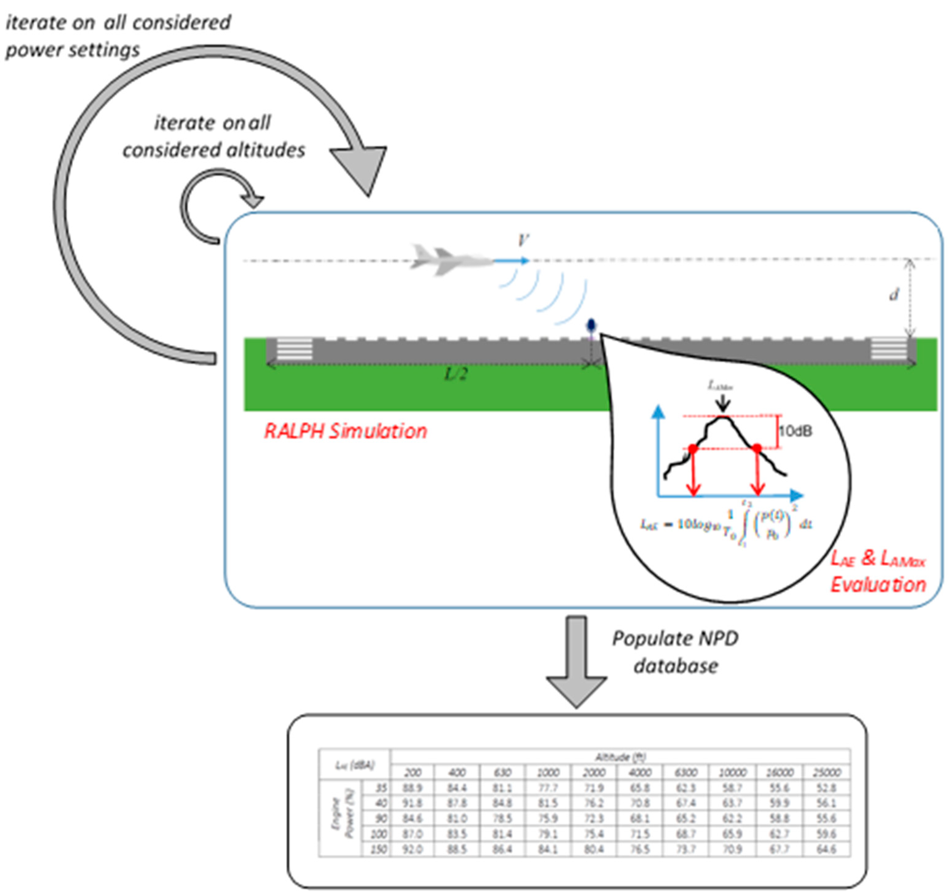
• Generation of noise–power–distance database through a ray-tracing approach;
• Acoustic impact at airport level evaluation with Aviation Environmental Design Tool (AEDT) procedure.

2. The Numerical Solvers

2.1. Aerodynamic Solver

The aerodynamic simulations were carried out by using the medium-fidelity code RAMSYS [5], which is an unsteady, inviscid, and incompressible free-wake vortex lattice boundary element methodology (BEM) solver for multi-rotor, multi-body configurations developed at CIRA and validated in several works [6,7,8]. It is based on Morino’s boundary integral formulation [9], for the solution of Laplace’s equation for the velocity potential φ. The surface pressure distributions are evaluated by applying the unsteady version of Bernoulli’s equation, which is then integrated to provide the forces and moments on the whole configuration and its components. A computational acceleration is obtained by applying the parallel execution via the OpenMP Application Programme Interface, and the module for symmetrical flows and geometries implemented in the solver.

2.2. Aeroacoustic Solver

The aeroacoustic simulations were carried out by using the ACOustic suite developed at CIRA and consisting of several tools for the evaluation of noise generation and propagation, presented and validated in [10,11,12,13].

In particular, the ACO-FWH solver is used for computing the acoustic free-field generated by the rotor blades. It is based on the FW–H formulation. The advanced-time formulation of Farassat 1A is employed, and the linear terms (the so-called thickness and loading noise contributions) are computed through integrals, on both the moving blades’ surfaces (impermeable/rigid surface formulation). Moreover, the space derivatives of the linear terms are also evaluated through both a numerical integration and the theoretical formulation developed by Lee. The quadrupole contribution due to the nonlinear terms distributed in the perturbed field around the blade is neglected. The computational acceleration is obtained by a parallel execution.

Starting from the unsteady aerodynamic blade surface pressure distributions, the results of the CIRA aerodynamic BEM code RAMSYS, the tonal noise components, were computed on a hemispheric surface encompassing all acoustic energy propagating in the downward direction.

2.3. NPD Calculation Methodology

The numerical methodology for the calculation of the NPD data of a given aircraft, simply considers simulations of flyovers of the given aircraft, properly acoustically characterized, in compliance with the regulation proposed by Society of Automotive Engineers SAE [3] for the calculation of airplane noise in the vicinity of airports. Each of the numerical simulations considers the acoustic source flying along a straight trajectory above a hypothetical runaway at a fixed altitude and with a given engine-power setting. By varying the altitude and engine-power settings, it is possible to fill a database that can correlate the value of sound exposure levels (L_AE) or effective perceived noise level (EPNL), in the centre of the hypothetical runaway, to each couple (engine-power setting, altitude) [14,15]. Also, the peak value of A-weighted instantaneous sound level, L_AMax, and the tone-corrected perceived noise level maximum value, PNLTM, are desirable in order to have a complete acoustic data set. This very fast and analytical methodology is able to simulate an expansive experimental campaign and provides the NPD curves for the Integrated Noise Model INM and/or Aviation Environmental Design Tool AEDT [2].

The process of populating a table similar to

Table 1. Example of NPD data.

LAE (dBA)		Altitude (ft)
		200	400	630	1000	2000	4000	6300	10,000	16,000	25,000
Engine Power (%)	35	88.9	84.4	81.1	77.7	71.9	65.8	62.3	58.7	55.6	52.8
	40	91.8	87.8	84.8	81.5	76.2	70.8	67.4	63.7	59.9	56.1
	90	84.6	81.0	78.5	75.9	72.3	68.1	65.2	62.2	58.8	55.6
	100	87.0	83.5	81.4	79.1	75.4	71.5	68.7	65.9	62.7	59.6
	150	92.0	88.5	86.4	84.1	80.4	76.5	73.7	70.9	67.7	64.6

is carried out by means of the RALPH code described in [4] and, in Figure 1, the process of the NPD evaluation is graphically represented.

To better reproduce a real measurement campaign for building the NPD database, some constraints were given for trajectories and all consequent calculations. First, the acoustic source, representing the given aircraft, is assumed to be precisely flying at a constant speed of 160 kts (82.31 m/s). Moreover, the timestamp for the trajectory evaluation is no longer than 0.5 s, to allow the acoustic parameters to be evaluated with a time-window of exactly 0.5 s, fulfilling the corresponding standard [3].

The RALPH code was configured to take into account the following phenomena and signal-processing options [14]:

• Ground reflection was active, and considered a perfect reflector;
• The Doppler effect ws active, to better consider the consequent atmospheric absorption;
• Atmospheric absorption was active, in fulfillment of the SAE-ARP 866B standard [16];
• A-weighting for the source spectra was active, in fulfillment of SAE AIR 1845 [3], for the NPD calculation.

Finally, it is worthy to remember that RALPH code does not consider obstacles, to date, and supposes perfectly flat terrain. These hypotheses are perfectly compliant with the actual scenario of an airport in the area of a runaway.

As already assessed, NPD databases were built both in terms of L_AMax and L_AE for all the considered configurations of the aircraft. Further data important to remark upon relates to the acoustic source. It is represented by a hemisphere (see [13] for more details) of radius 100 m. The importance of this data will be clear in the next section, as the acoustic effect produced by the source is only valid outside the hemisphere.

2.4. AEDT Approach and Regulations

As reported in [17], the Federal Aviation Administration, Office of Environment and Energy (FAA-AEE) developed Aviation Environmental Design Tool AEDT to evaluate aircraft noise and emissions for airport environmental studies. This model has replaced the legacy noise model, the Integrated Noise Model (INM) and the emission model, Emissions and Dispersion Modeling System (EDMS). Although there is significant overlap in functionality and underlying methodology between the AEDT and legacy tools, AEDT has a fundamentally different system architecture, design, and capabilities, which allow the user to simultaneously model aviation noise, fuel consumption, and emissions within a common interface and from common inputs.

Noise regulation, at the Italian national level, observes the directive: “Legge Quadro sull’Inquinamento Acustico n. 447 del 26/10/95” [18], which regulates noise-pollution matters. The norm establishes the general context and leaves to successive decree-laws the definition of the technical and operating parameters.

The Ministerial Decree of 31 October 1997 “Airport noise measurement methodology” [19] is used as a reference in the assessment of airport noise and, more precisely, in the airport noise assessment index (LVA). This parameter, adopted for the determination of the noise contour maps, is expressed in dB(A) and is calculated in accordance with Annex A of that decree.

At the community level, Legislative Decree 194/05 [20] transposes the European Directive on environmental noise 2002/49 to the Italian context. This Decree introduces two new descriptors [21]: L_DEN and L_Night. L_DEN is the day–evening–night noise level and it is an indicator of the overall noise nuisance over an entire 24-h period. It is constructed by combining, in “weighted” mode, the L_Day, L_Evening and L_Night levels (representing the A-weighted equivalent continuous long-term levels over the entire day, evening, night periods—respectively—for a calendar year). L_Night is the level of night noise, which also considers the calculation of the indicator L_DEN, and represents the equivalent long-term equivalent continuous level A-weighted over all the nights of a calendar year. L_Night is an indicator relevant to sleep-induced disorders. The day–evening–night period is from 6.00 to 6.00 the next day and is divided into the following time slots:

• day period: from 06.00 to 20.00;
• evening period: from 20.00 to 22.00;
• night period: from 22.00 to 06.00.

The acoustic descriptors, L_DEN and L_Night, are used to draw acoustic maps and strategic acoustic maps. The two descriptors are defined in Annex I of the Directive. In particular, the level L_DEN, in decibels (dB), is defined by the following formula:

$$L_{DEN}=10·{\log }_{10}\left[\frac{14}{24}·\left({10}^{\frac{Lday}{10}}\right)+\frac{2}{24}·\left({10}^{\frac{Levening+5}{10}}\right)+\frac{8}{24}·\left({10}^{\frac{Lnight+10}{10}}\right)\right]$$

(1)

where:

$$\begin{gathered} L_{Day}=10·{\log }_{10}\left[\frac{t_0}{T_0}{\displaystyle \sum }_{i=1}^{N_{day}}{10}^{\frac{L_{AEi}}{10}}\right] \\ {L}_{Evening}=10·{\log }_{10}\left[\frac{t_0}{T_0}{\displaystyle \sum }_{i=1}^{N_{evening}}{10}^{\frac{L_{AEi}}{10}}\right] \\ {L}_{Night}=10·{\log }_{10}\left[\frac{t_0}{T_0}{\displaystyle \sum }_{i=1}^{N_{night}}{10}^{\frac{L_{AEi}}{10}}\right] \end{gathered}$$

• T₀ is the product of the number of seconds of the part of the day for which the descriptor is defined and the number of days, N_Tr, for which basic-scenario air traffic is defined (in this case N_Tr = 365);
• N_day,N_evening, and N_night are the aircraft noise events that occur during the specified reference time period, T₀;
• t₀ is the reference time of 1 s.
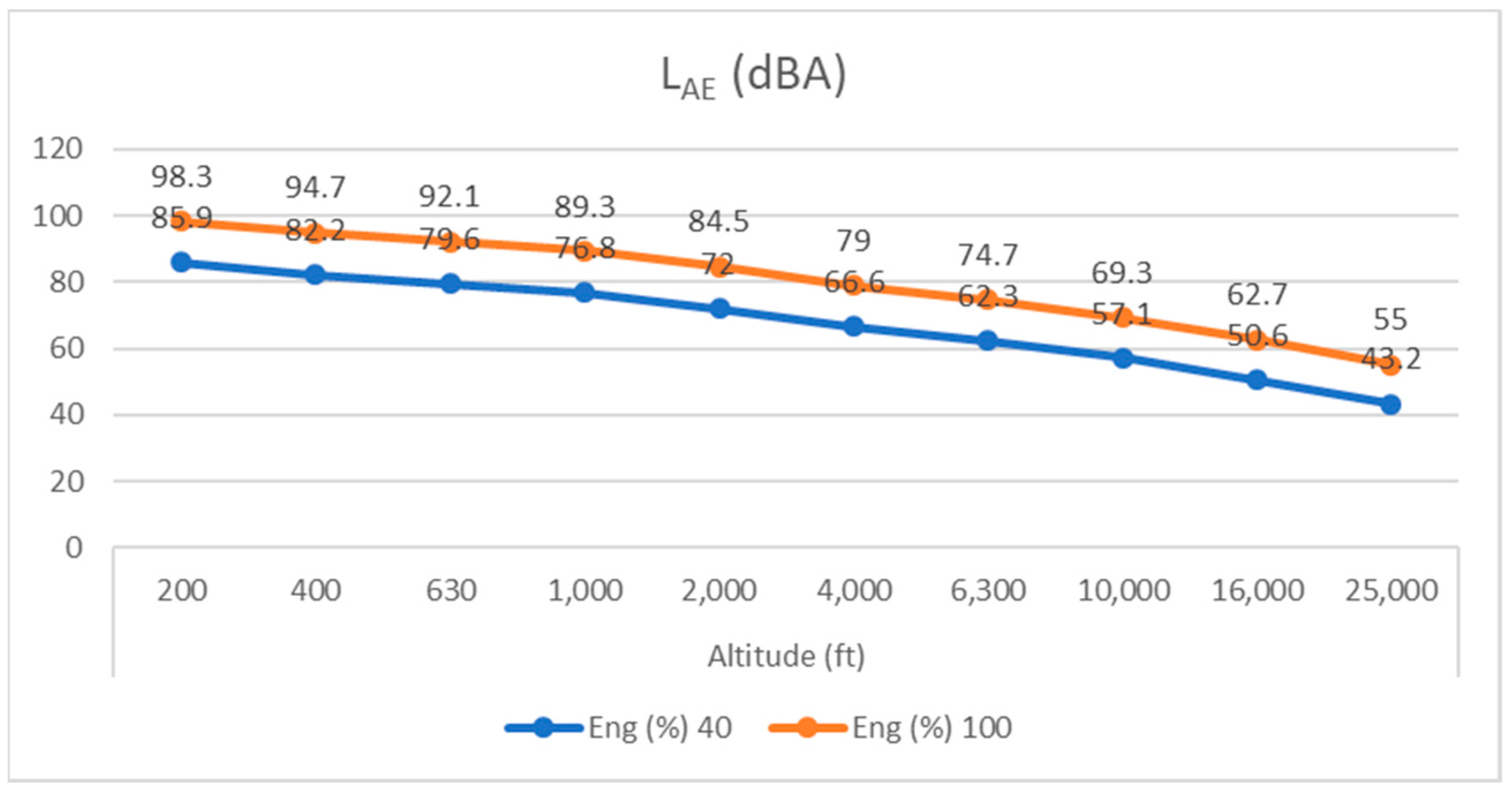
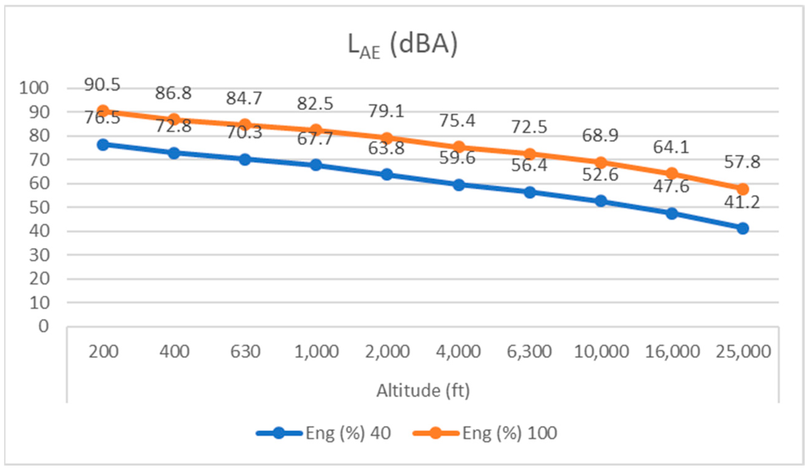
• L_AE is the A-weighted sound exposure level (SEL), defined as the constant sound level having the same energy in one second as the original noise event, computed for the time during which the sound level is 10 dB below the maximum level:

$$L_{AE}=10·{\log }_{10}\left[\frac{1}{t_0}{\displaystyle \sum }_{i=t1}^{t_2}{10}^{\frac{L_{AFi}}{10}}\right]$$

(2)

where (t₂ − t₁) is the time interval during which the L_AF level remains above the L_AFmax value, −10 dB.

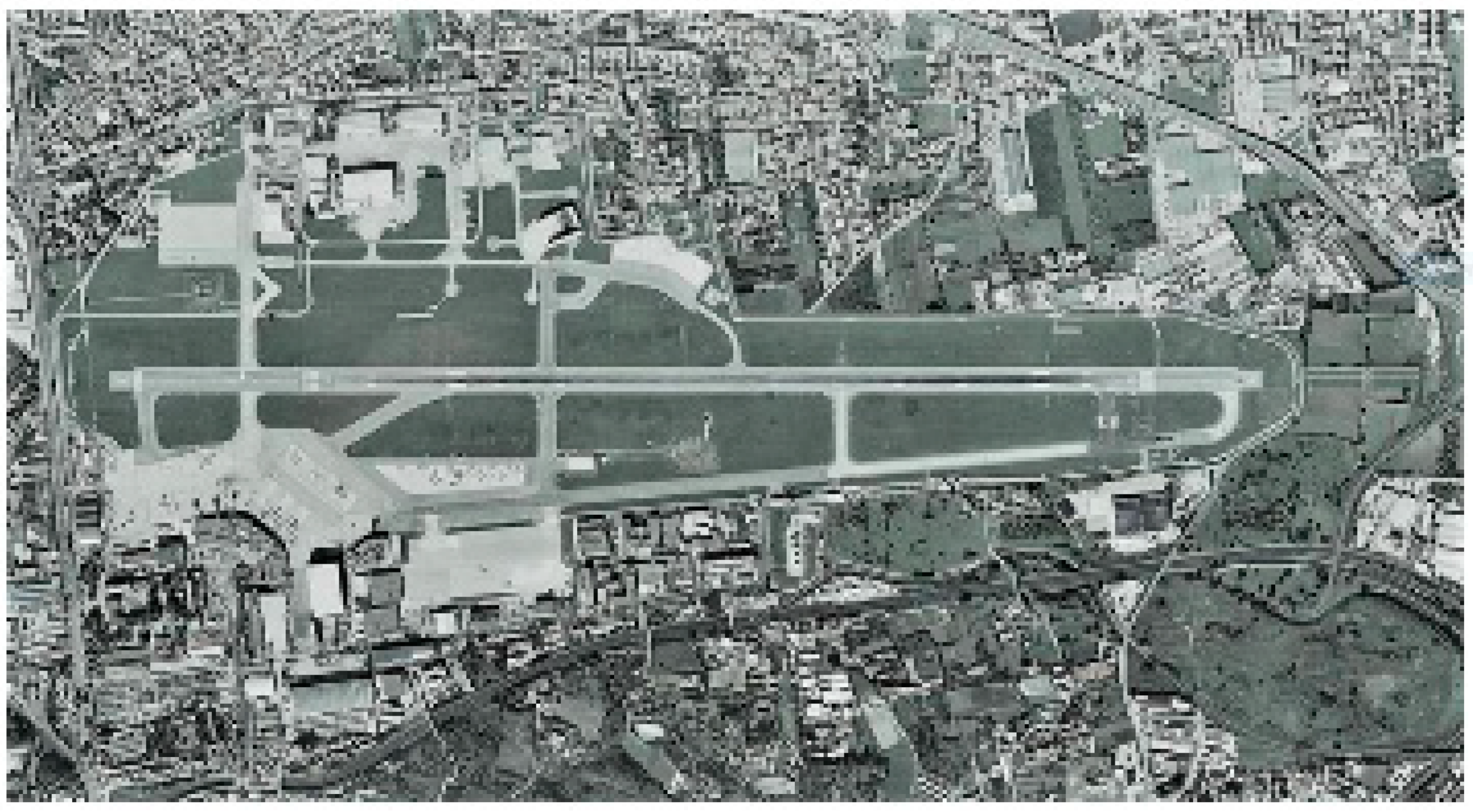
2.4.1. Selected Airport: Naples’ “Ugo Niutta Capodichino” Airport

The international airport of Naples, Capodichino, is the first airport in Southern Italy and its fifth national airport; its IATA code is NAP and its ICAO code is LIRN in Class4D.

It is located about 4 km from the central station of Naples. The runway size is 2.628 × 45 mt, composed of bitmac and concrete. The altitude of the airport is 90 mt and its GPS coordinates are (40°53′04″ N, 14°17′27″ E). Figure 2 depicts an image of Capodichino airport.

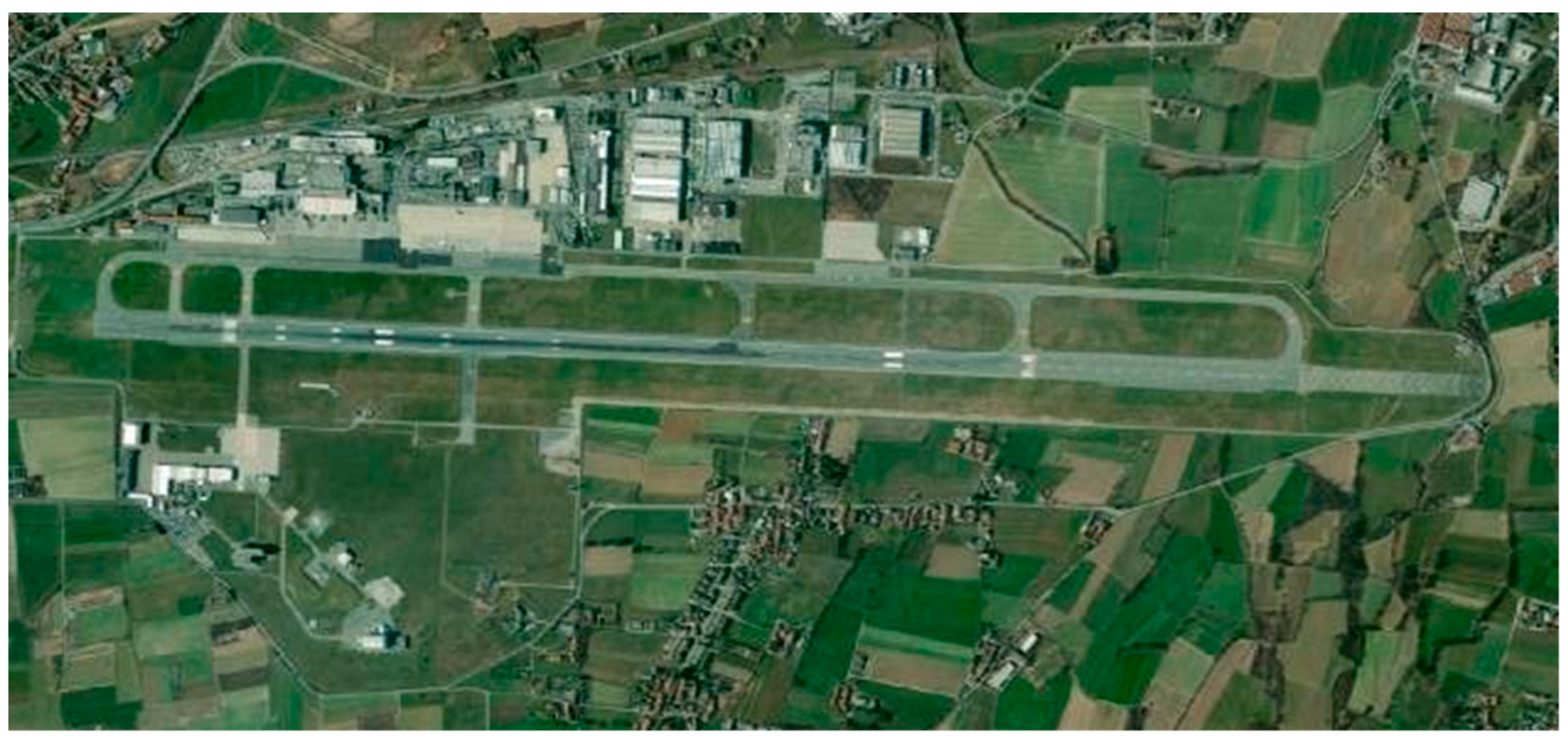
2.4.2. Selected Airport: Turin’s “Turin-Caselle” Airport

Turin-Caselle Airport is an airport located at Caselle Torinese, 16 km (9.9 mi) north-northwest of the city of Turin, in the Metropolitan City of Turin, Piedmont region, northern Italy. It is also named Sandro Pertini Airport. Its IATA code is TRN and its ICAO code is LIMF in Class4E.

Its runway size is 3300 × 60 mt and composed of bituminous conglomerate. The altitude of the airport is 302 mt and its GPS coordinates are (45°12′09″ N, 7°38′58″ E). Figure 3 depicts an image of Caselle airport.

3. Description of the Aircraft Configurations

Two configurations, based on the ATR42 regional aircraft, were investigated. The aircraft models were provided by the University of Naples, which was also involved in the project PROSIB.

The baseline configuration is named “Configuration A”. This configuration consisted of a simplified version of the regional aircraft ATR42 geometry, as in Figure 4.

The hybrid-electric configuration is named “Motorization 2”. This configuration consisted of a modified version of the regional aircraft ATR42, having a new wing of equal length and higher aspect ratio, two tip propellers to reduce induced drag, and a distributed electric propulsion (DEP) system, composed of four propellers per side, as in Figure 5. This configuration was selected among several proposal aircraft generated and investigated by our partner, the University of Naples [22].

The propellers of the two configurations were designed and optimized by CIRA during another phase of the PROSIB project [23].

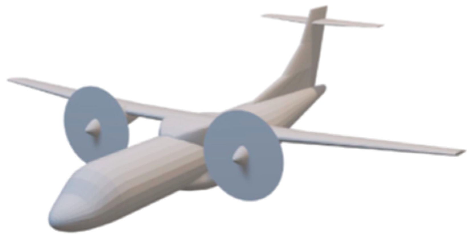
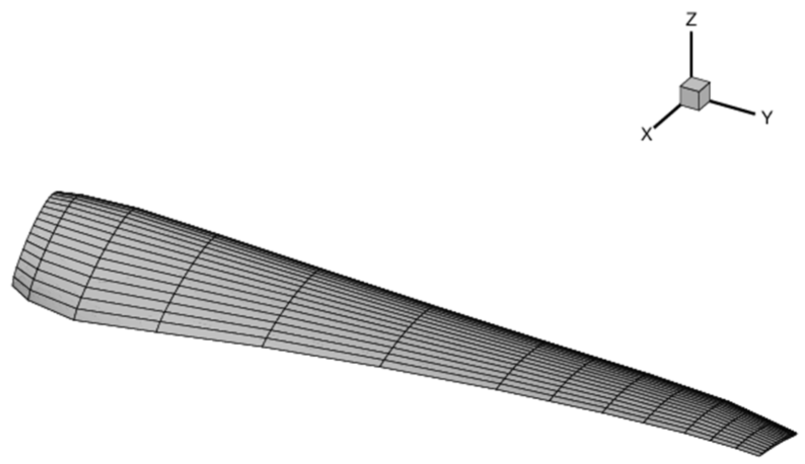
3.1. Baseline Configuration (Configuration A): Propeller

The propeller was completely re-designed and optimized by CIRA and therefore was different from the original one installed on the ATR42 aircraft. It consisted of four blades having length equal to 1.965 m and was equipped with feathering hinges for each blade. The hub was not modelled. The sense of rotation of the two propellers was counterclockwise when viewed from the front of the rotor disk.

Each blade geometry was discretized by 40 chordwise panels × 13 spanwise panels. The resulting rotor blade geometry is shown in Figure 6.

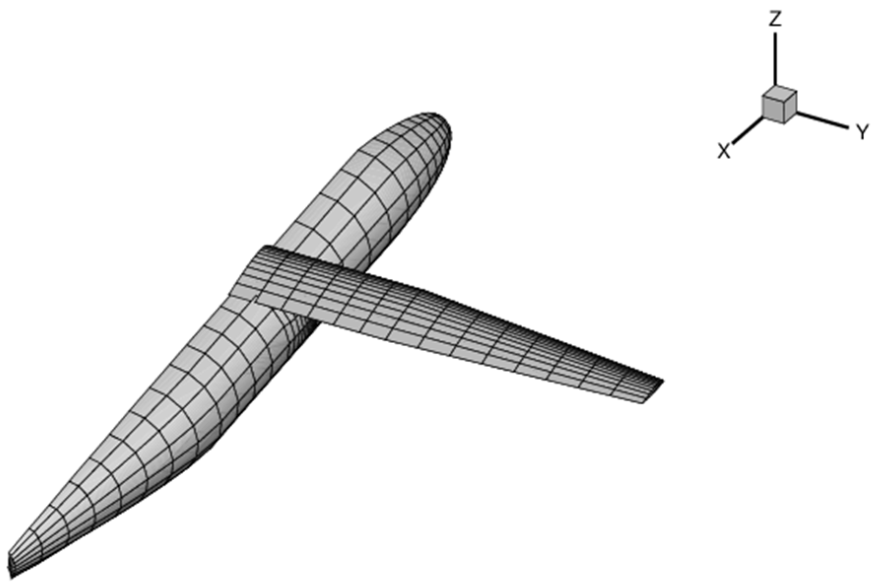
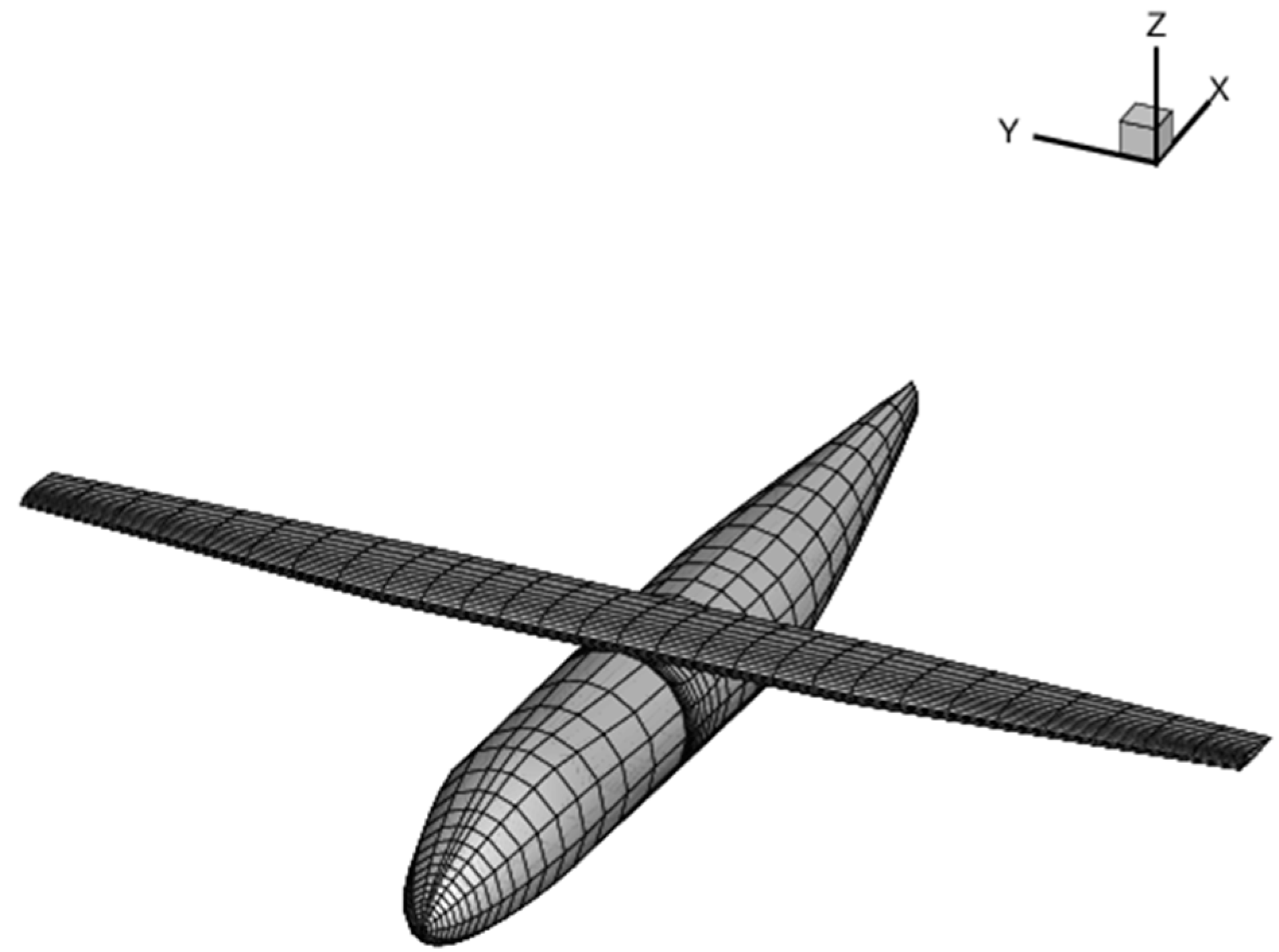
3.2. Baseline Configuration (Configuration A): Airframe

The CAD file of the airframe is illustrated in Figure 7. The geometry was simplified by omitting the empennages, both vertical and horizontal, considered to have a negligible effect on the tonal noise generated by the aircraft, and the nacelles.

The geometry was then discretized by using six patches, for a total of 1528 panels, as shown in Figure 8.

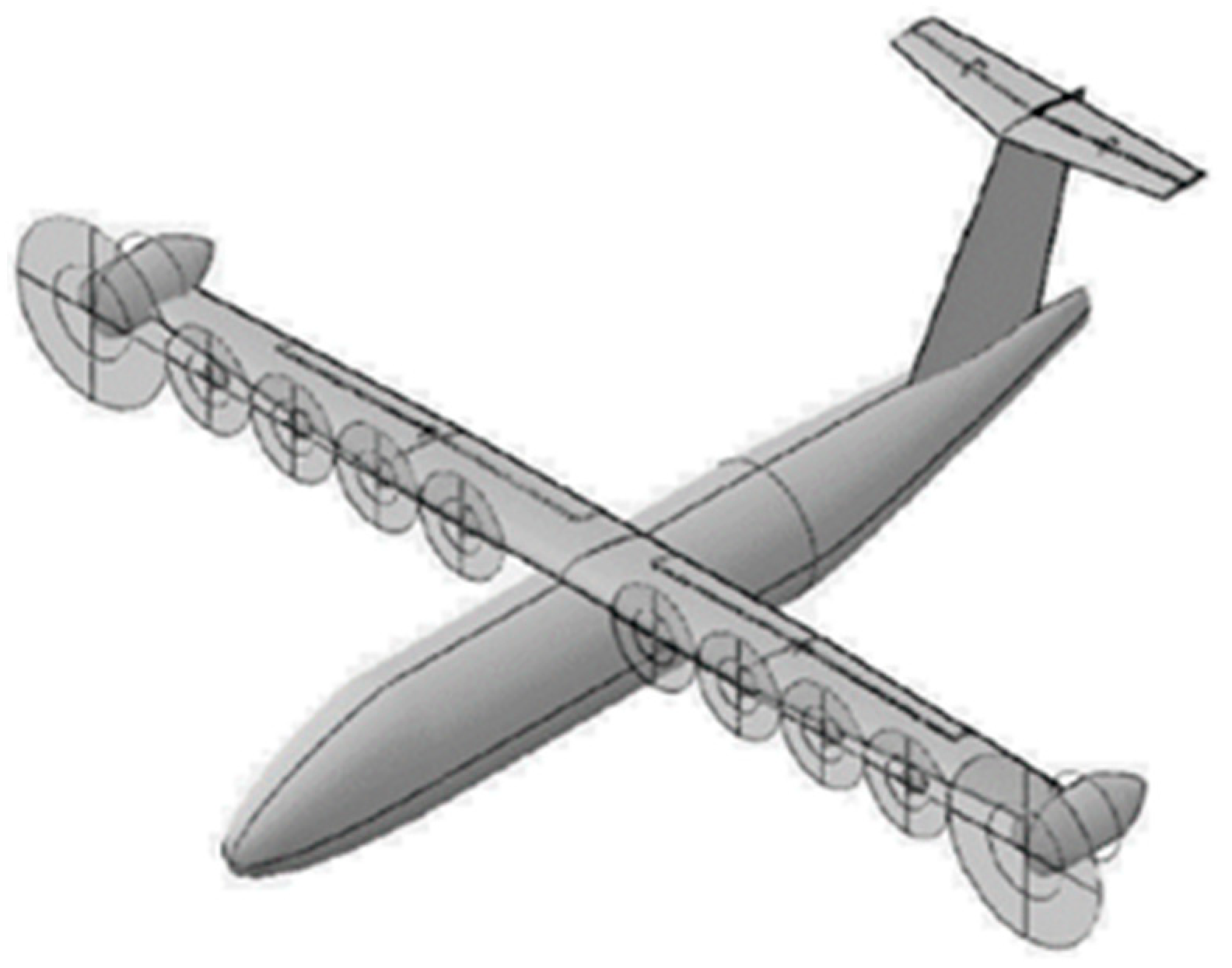
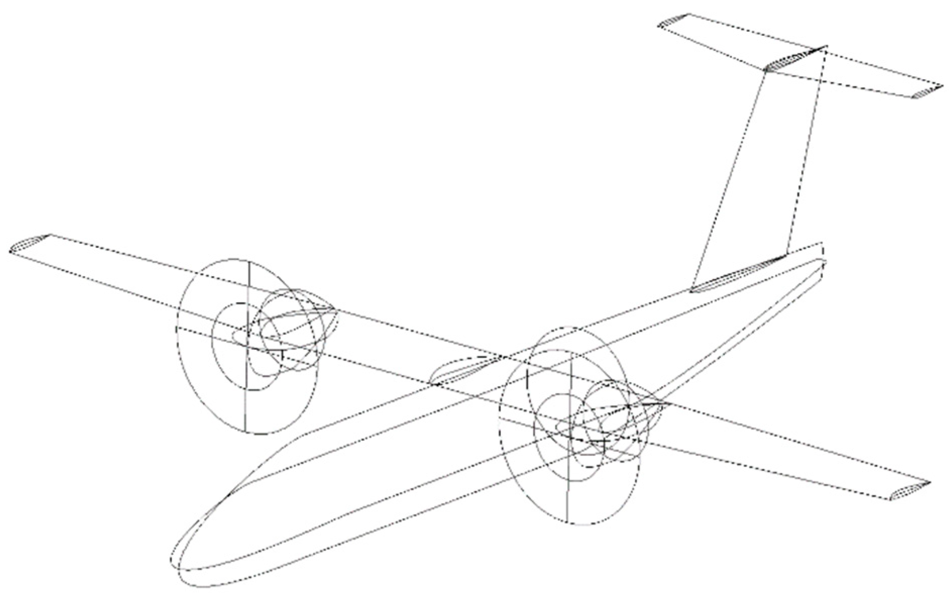
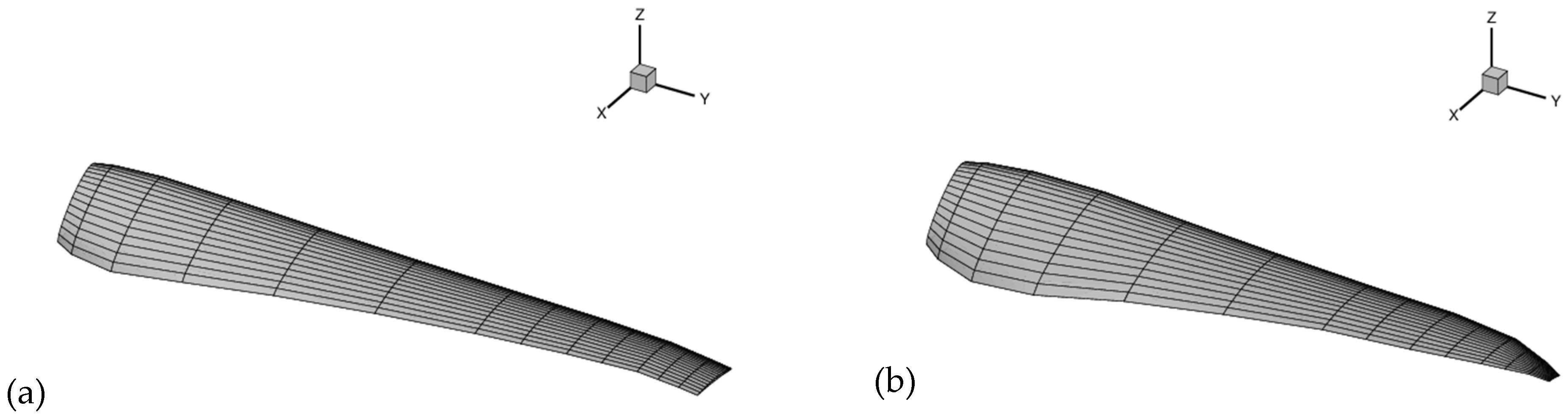
3.3. Hybrid-Electric Configuration (Motorization 2): Propeller

The propellers were designed and optimized by CIRA. The tip propeller consisted of four blades having length equal to 1.965 m and was equipped with feathering hinge for each blade. The hub was not modelled. The sense of rotation of the starboard-side propeller, selected as the reference one, was counter-clockwise when viewed from the front of the rotor disk. Each blade geometry was discretized by 40 chordwise panels × 13 spanwise panels. The resulting rotor blade geometry is shown in Figure 9a.

Each of the four DEP propellers consisted of six blades having length equal to 1.100 m. The blade pitch was fixed. The hub was not modelled. The sense of rotation of the starboard-side propellers, selected as the reference one, was counter-clockwise when viewed from the front of the rotor disk. Each blade geometry was discretized by 40 chordwise panels × 13 spanwise panels. The resulting rotor blade geometry is shown in Figure 9b.

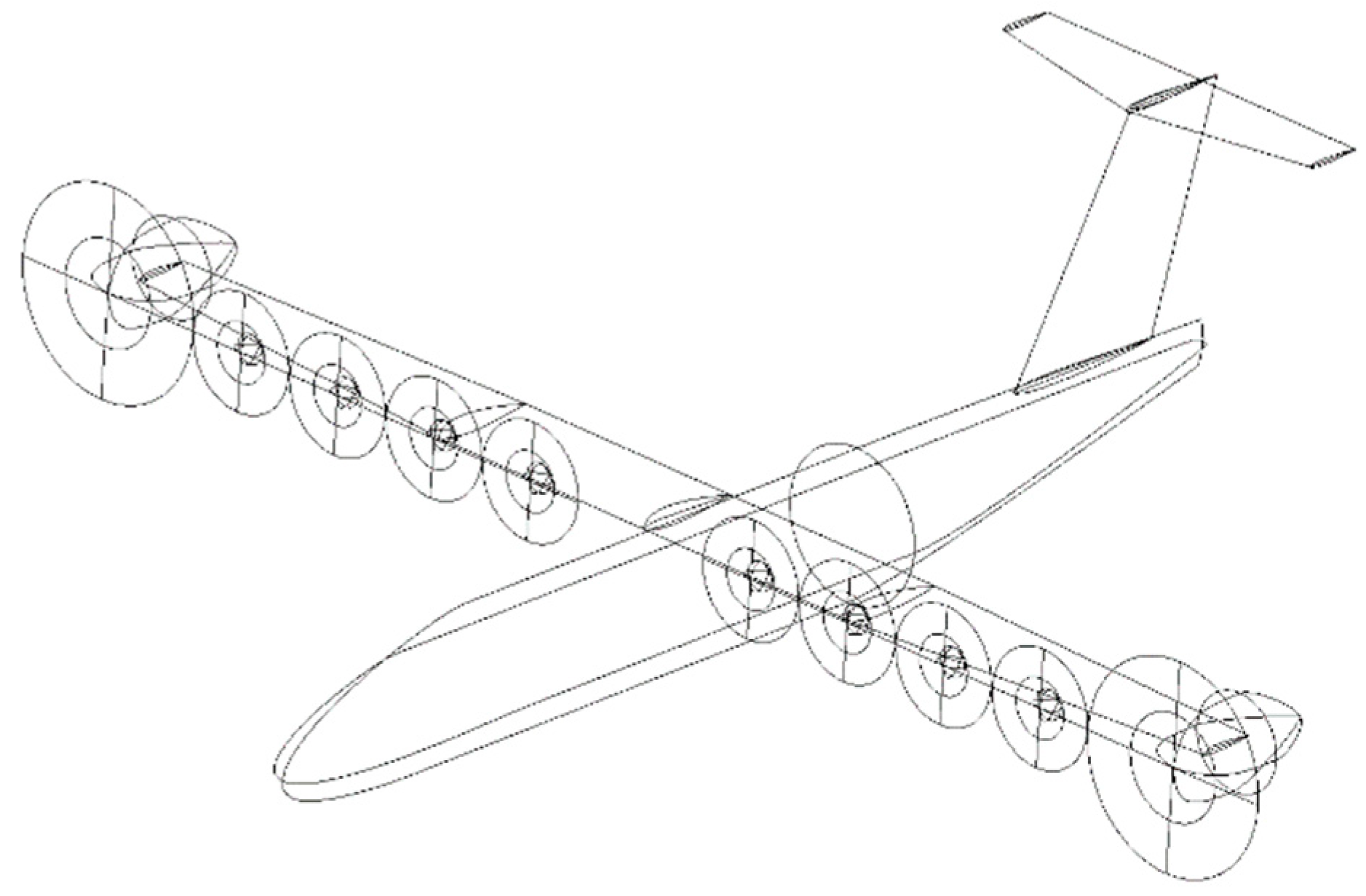
3.4. Hybrid-Electric Configuration (Motorization 2): Airframe

The CAD file of the airframe is illustrated in Figure 10. The geometry was simplified by omitting the empennages, both vertical and horizontal, considered to have a negligible effect on the tonal noise generated by the aircraft, and the nacelles.

Since the flight conditions investigated were fully symmetric and the propellers were all in-phase and contra-rotating, the modelling of just half the airframe was performed, which was then discretized by using two patches for a total of 716 panels, as shown in Figure 11.

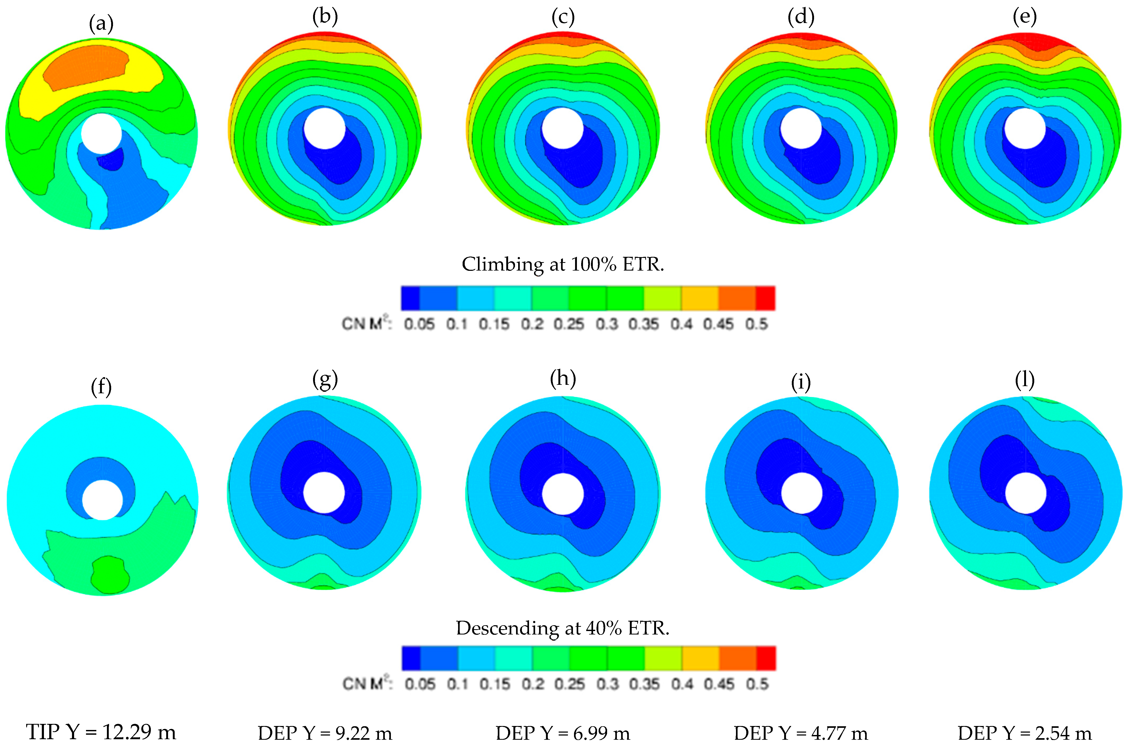
3.5. Description of the Test Conditions for the Hemisphere Generation

For each of the two configurations investigated, two flight conditions were considered: climb, at 100% ETR (full thrust), and descent, at 40% ETR. In all calculations the speed of flight and the altitude were set at 160 kts and 1000 ft, respectively.

Table 2. Main characteristics—Config. A.

	AoA [deg]	T [N]	T Total [N]
Climb	5.50	20,985	41,969.82
Descent	−2.00	8394	16,787.93

and

Table 3. Main characteristics—Mot. 2.

	AoA [deg]	T Tip [N]	T DEP [N]	T Total [N]
Climb	9.00	2886	6493	57,718.22
Descent	−2.00	1154	2597	23,087.29

summarize the main characteristics of the flight conditions for the two configurations, in terms of Angle of attack (AoA), trust of single propeller (T) and total trust of all propellers (T Total).

The propellers’ speed, in Configuration A, were set to 1200 RM for both flight conditions.

The reduction in thrust was obtained by changing the collective pitch ${\theta }_0$. In particular, it was set to 35.91° for climbing flight, and to 26.63° for descending flight.

In the case of Motorization 2, the nominal values for the propellers’ speeds were selected in 100%-ETR climbing flight only. An adjustment in pitch was necessary in order to obtain nominal thrust from each propeller. The revolutions per minute RPMs and resulting collective pitch angles ${\theta }_0$ are summarized in

Table 4. Mot. 2: Propellers’ RPM and collective pitch in a 100%-ETR climb.

Propeller	RPM	Y Span [m]	θ0 [deg]
DEP 1	1520	2.5440	47.10
DEP 2	1520	4.7685	47.08
DEP 3	1520	6.9930	47.64
DEP 4	1520	9.2175	47.90
TIP	1158	12.2900	19.88

.

In descending flight, the reduction in thrust to 40% ETR for the DEP propellers was only possible via a reduction in RPM. Instead, the required thrust reduction for the tip propellers was produced by reducing the propeller speed to 1019 RPM and changing the collective pitch of the blades.

Table 5. Mot. 2: Propellers’ RPM and collective pitch in 40%-ETR descent.

Propeller	RPM	Y Span [m]	θ0 [deg]
DEP 1	1160	2.5440	47.10
DEP 2	1160	4.7685	47.08
DEP 3	1160	6.9930	47.64
DEP 4	1160	9.2175	47.90
TIP	1019	12.2900	22.10

summarizes the resulting RPMs and collective pitch angles ${\theta }_0$.

4. Analysis of the Results

4.1. Aerodynamic Results

All numerical simulations were carried out with a time resolution corresponding to an azimuth step of the reference propeller (portside propeller for Configuration A, innermost DEP propeller for Motorization 2) equal to 3°. Four propeller revolutions were required to reach a convergent periodic solution and four spirals were used to model the propellers’ wakes.

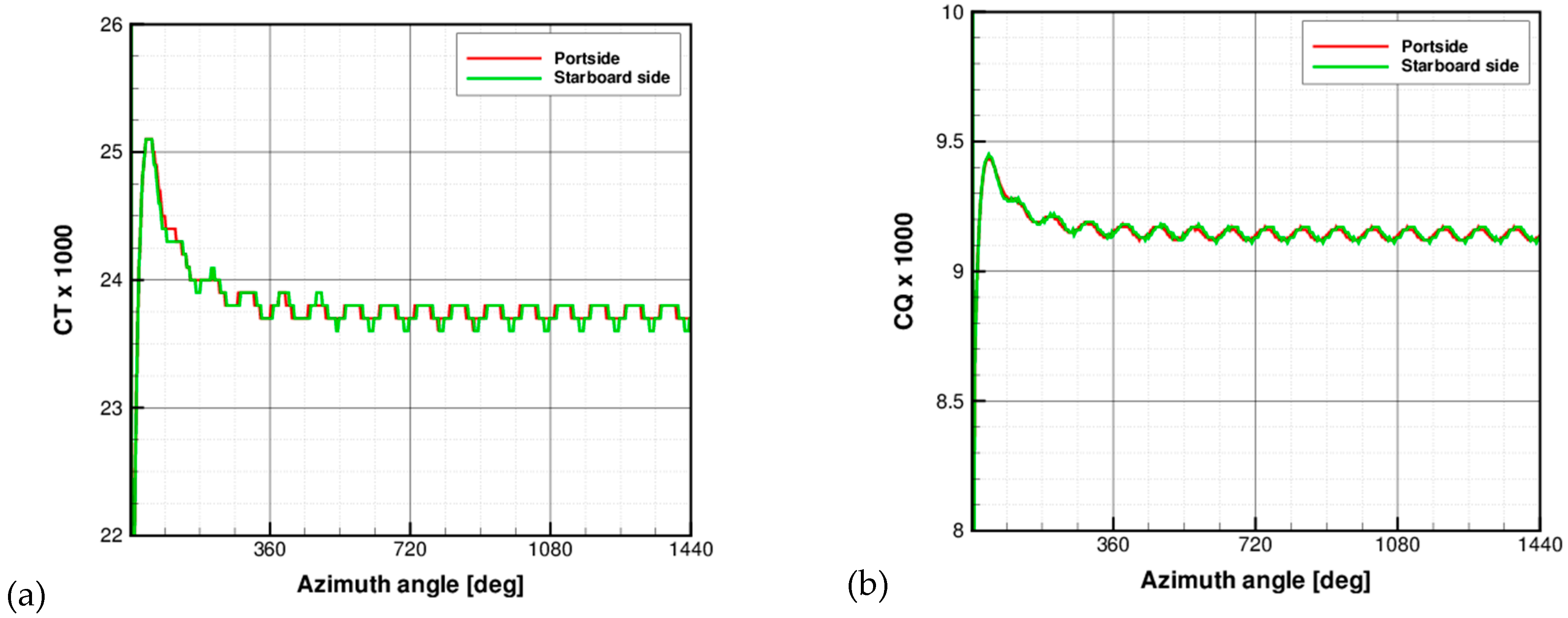
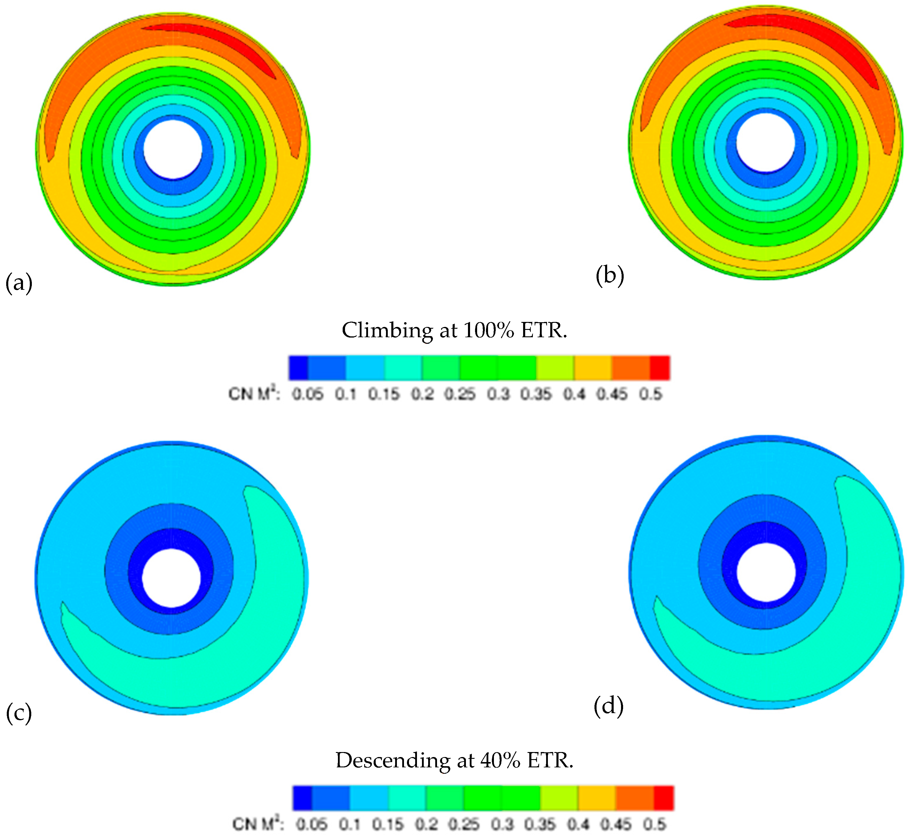
4.1.1. Configuration A

Figure 12 illustrates the interactional process between the propellers, their wakes, and the airframe. In particular, the pressure distributions on the wing highlight a concentrated peak expansion at the leading edge produced by the interaction with the propellers and their wakes.

An example of the convergence history of the solution is represented in Figure 13, for climbing flight at full thrust, in terms of the thrust and induced torque coefficients. The figure shows that the portside and starboard-side propellers have the same behavior.

Figure 14 shows a representation of the loads CN M² acting on the propellers’ disk both in climbing, at full thrust, and in descending flight, at 40% ETR. In particular, the higher loads on the upper region of the disks while climbing are mainly explained by the positive angle of attack (AoA) of the aircraft’s attitude. Only little differences can be observed between the loads of the two propellers. In descending flight, the load distribution is significantly reduced, because of the 40% ETR, and reversed with respect to climbing. Indeed, the negative attitude of the aircraft produces higher loads on the lower region of the propellers’ disks.

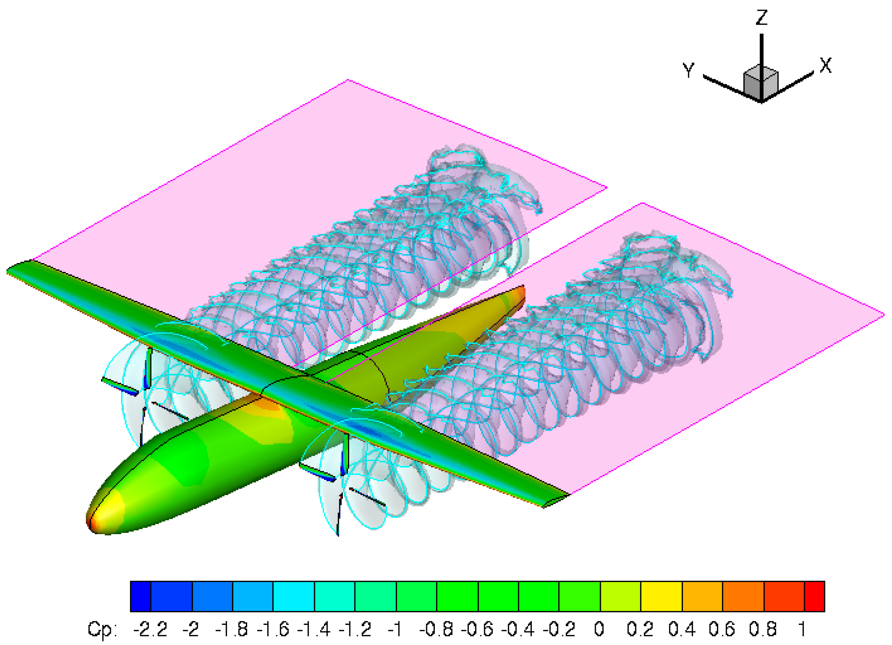
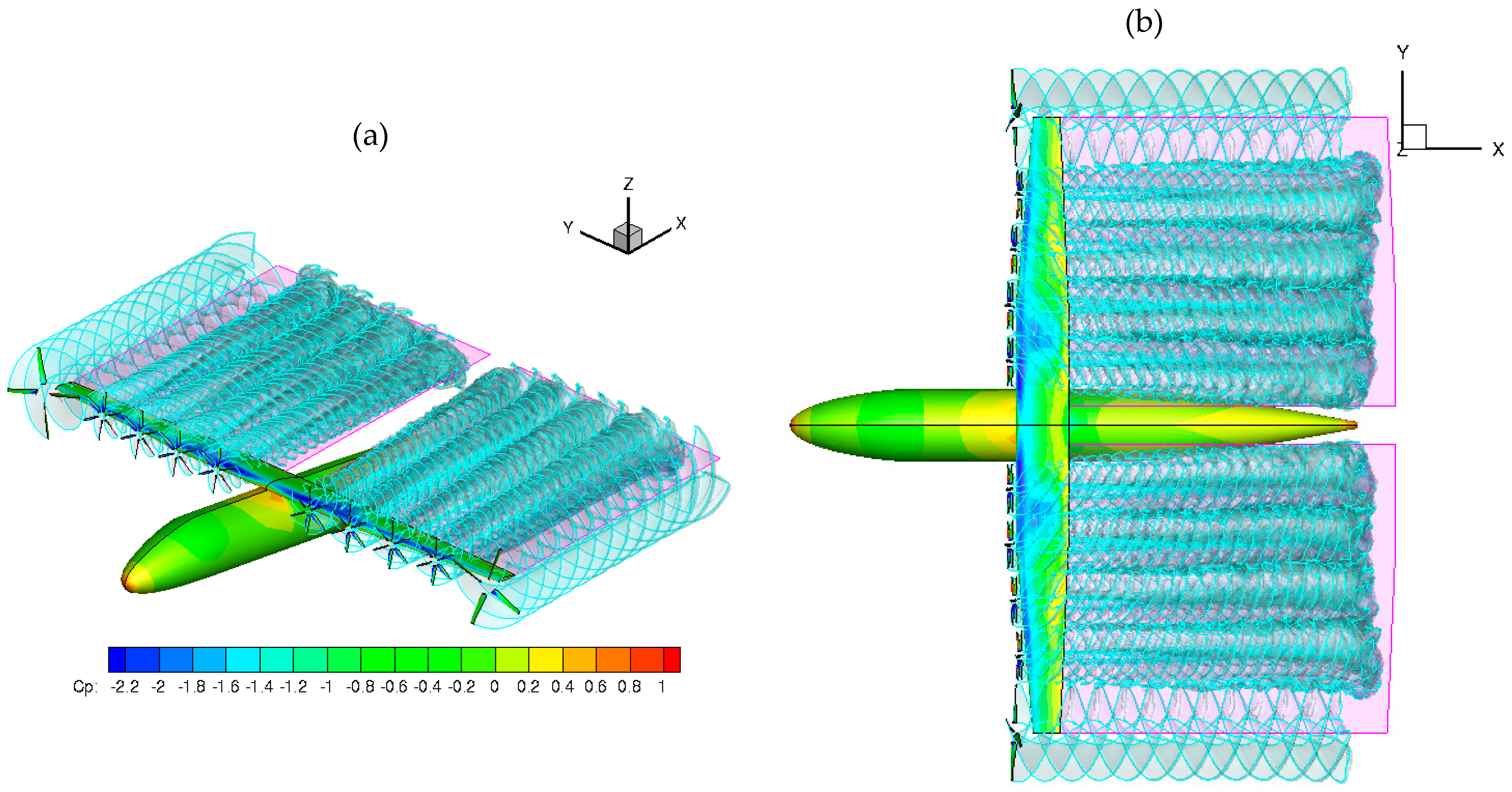
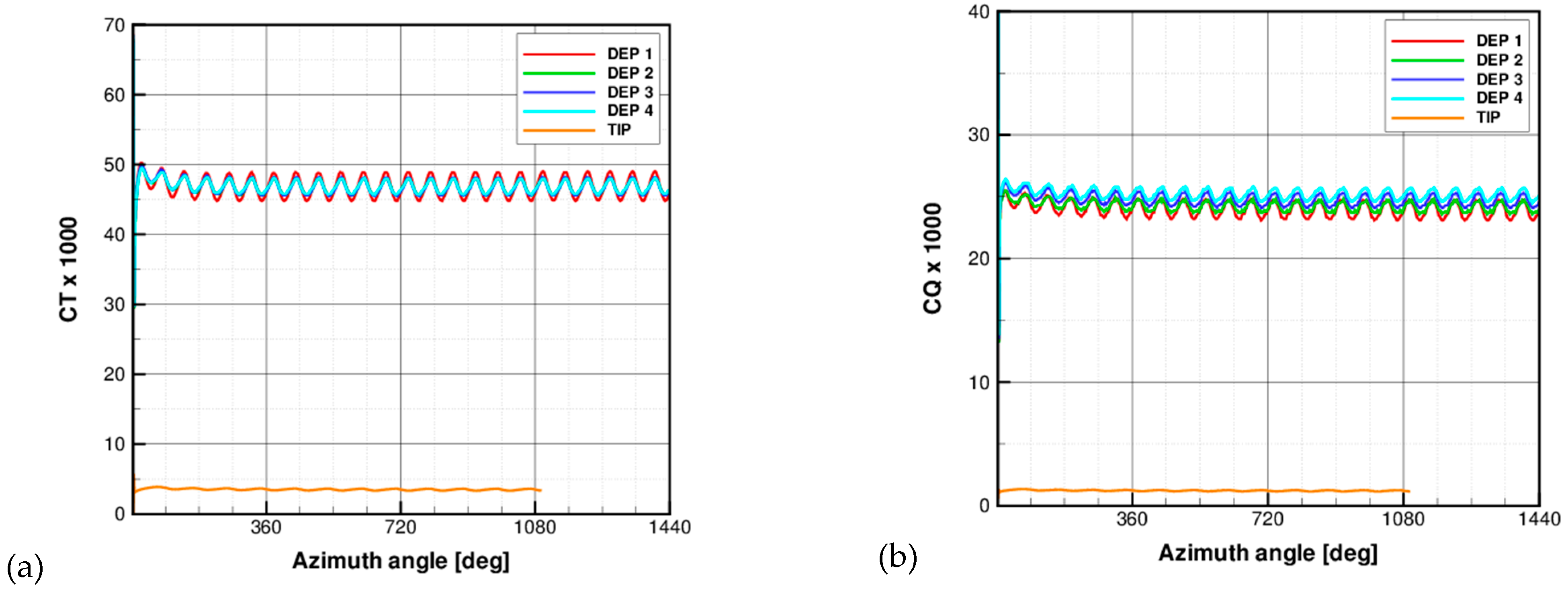
4.1.2. Motorization 2

Figure 15 illustrates the interactional process between the propellers, their wakes, and the airframe. In particular, the pressure distributions on the wing highlight a peak expansion at the leading edge throughout the wing, produced by the interactions with the propellers and their wakes. In particular, the top view highlights that the interactional effect of the DEP propellers is higher in the proximity to the fuselage and between the first two innermost DEP propellers, where the expansion extends to more than half the local chord length.

An example of the convergence history of the solution for climbing flight at full thrust is represented in Figure 16, in terms of the thrust and induced torque coefficients. The figure shows that the four DEP propellers produce the same average thrust with only a slight difference in amplitude for the DEP propeller closer to the tip propeller, DEP4. The propeller DEP1 (red line) is located near the fuselage and produces a thrust fluctuation that is slightly higher than the others due to its interaction with the fuselage on its side. extremely reduced thrust generated by the tip propeller was also observed. The difference in RPM between the DEP propellers and the tip one is such that four revolutions of the DEP propellers correspond to about three revolutions of the tip propeller. Finally, slight differences in the average values of the induced torque were also observed.

Figure 17 shows a representation of the loads, CN M², acting on the propellers’ disk both in climbing, at full thrust, and in descending flight, at 40% ETR. In particular, the higher loads on the upper region of the disks in climb are mainly explained by the positive AoA of the aircraft’s attitude. All DEP propellers show a similar behavior, with a localized region of low CN M² in the lower region of the disk and in the inner part of the blade span. The tip propeller produces much lower loads on the disk.

In descending flight at 40% ETR, the loads on the disks are significantly reduced. The load distributions show a wider area of lower values, bounding the higher values toward the blade tips, especially in the lower region of the disks. The negative attitude of the aircraft produces higher loads on the lower region of the tip propeller disk, resulting in a reversed behavior with respect to the climbing flight.

4.2. Aeroacoustic Results

The acoustic free-field was computed on a sphere of 100 m of radius, from the first through tenth blade passage frequencies (BPF). The acoustic solution was calculated in the time domain, by integrating the unsteady aerodynamic pressure on the blades through the solid formulation of the FW–H equation. Signals were post-processed through the fast Fourier transform formula and the frequency of the domain counterpart was stored in terms of complex acoustic pressure, p, and its normal derivative, dp/dn.

For both the Configuration A and Motorization 2 aircraft, the noise was evaluated in terms of overall sound pressure levels (OASPL) and overall A-weighted sound pressure levels (OASPL-A), to include the contribution of all the 10 BPFs.

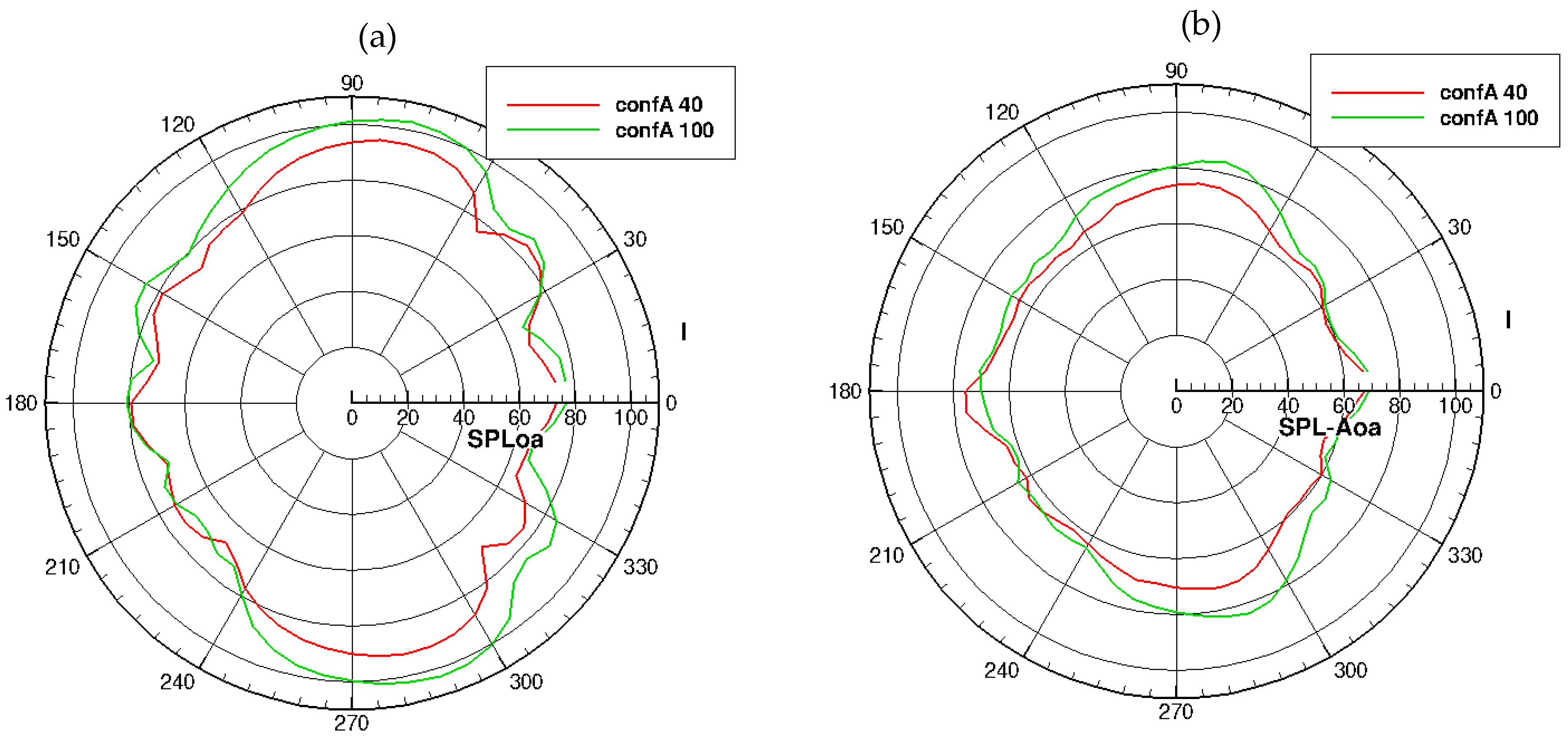
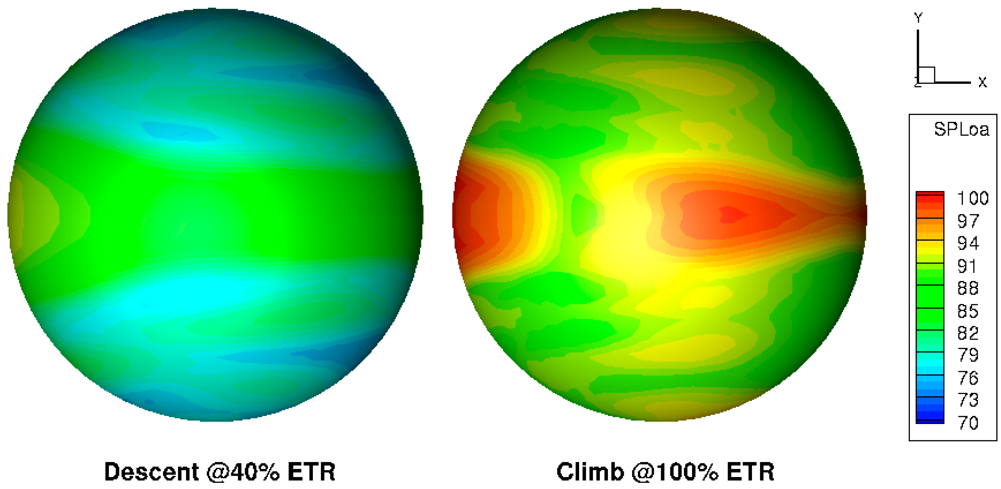
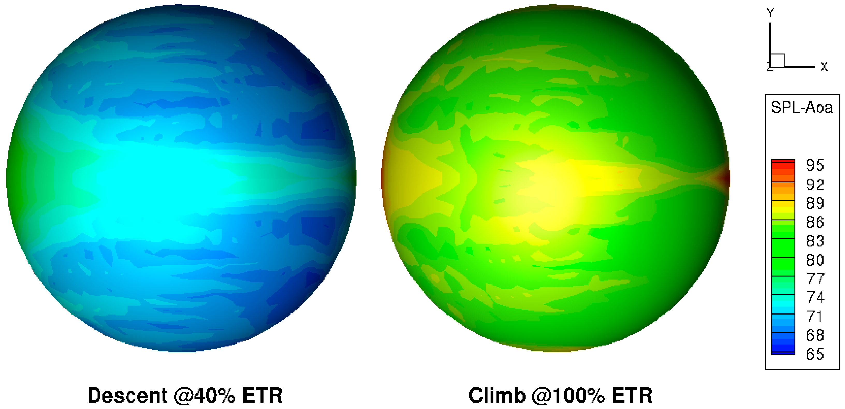
4.2.1. Configuration A

In Figure 18 and Figure 19, the overall SPL on the reference sphere surface is shown, for the aircraft Configuration A, in the two thrust conditions. As expected, the noise is more than 10 dB greater for the full thrust climb condition respect to descent condition. Looking at the noise field, the zones where the propellers are located, have the higher values of SPL. Similar results are in the plot of overall A-weighted SPL, which are more related to the effect of the highest BPFs.

To produce evidence of the differences between the noise levels in the two thrust conditions, Figure 20 shows the directivity diagrams in the horizontal plane XY centered in the position of the aircraft. The noise field is quite similar for both simulations, with greater values for the full thrust configuration.

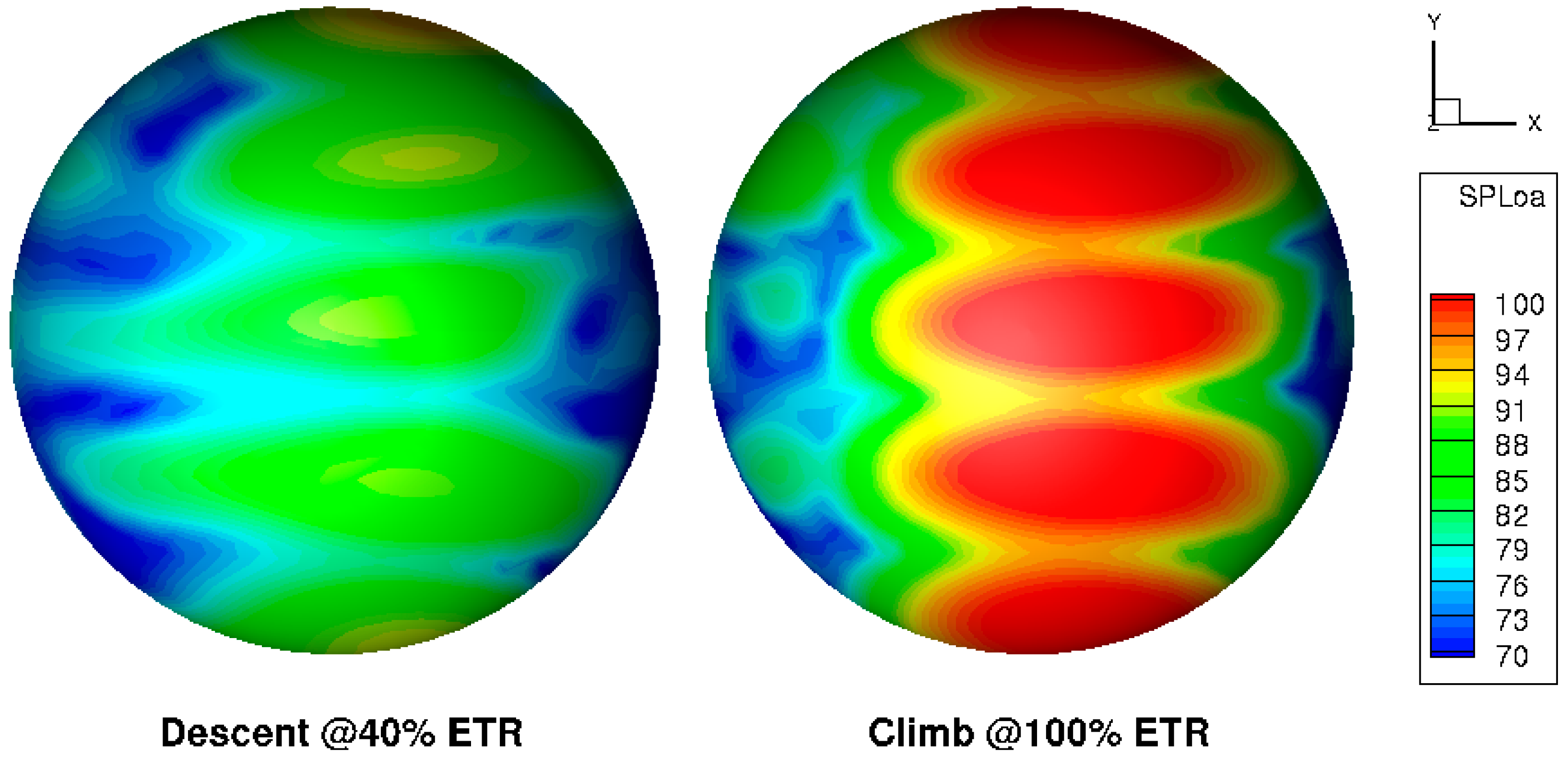
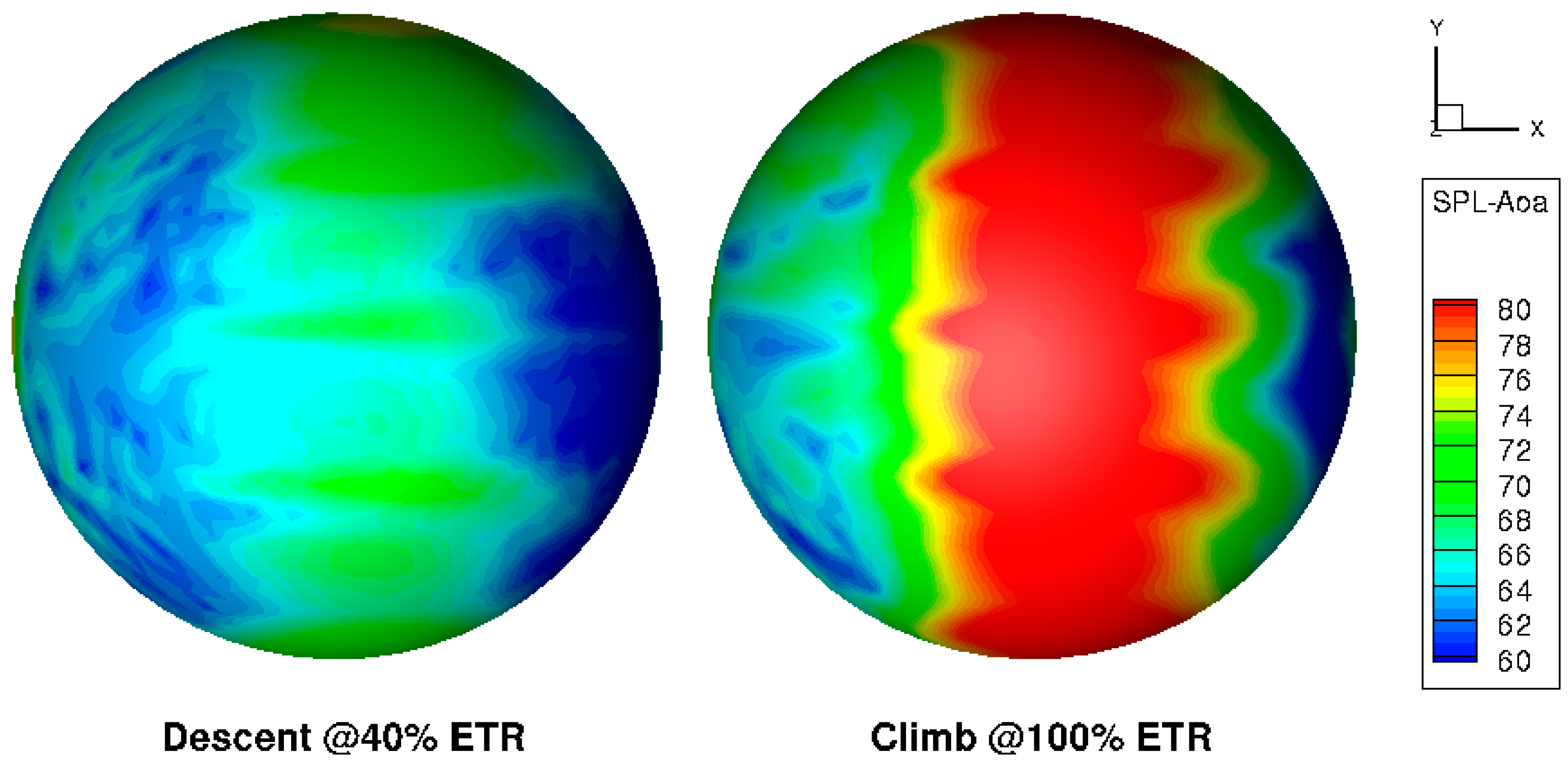
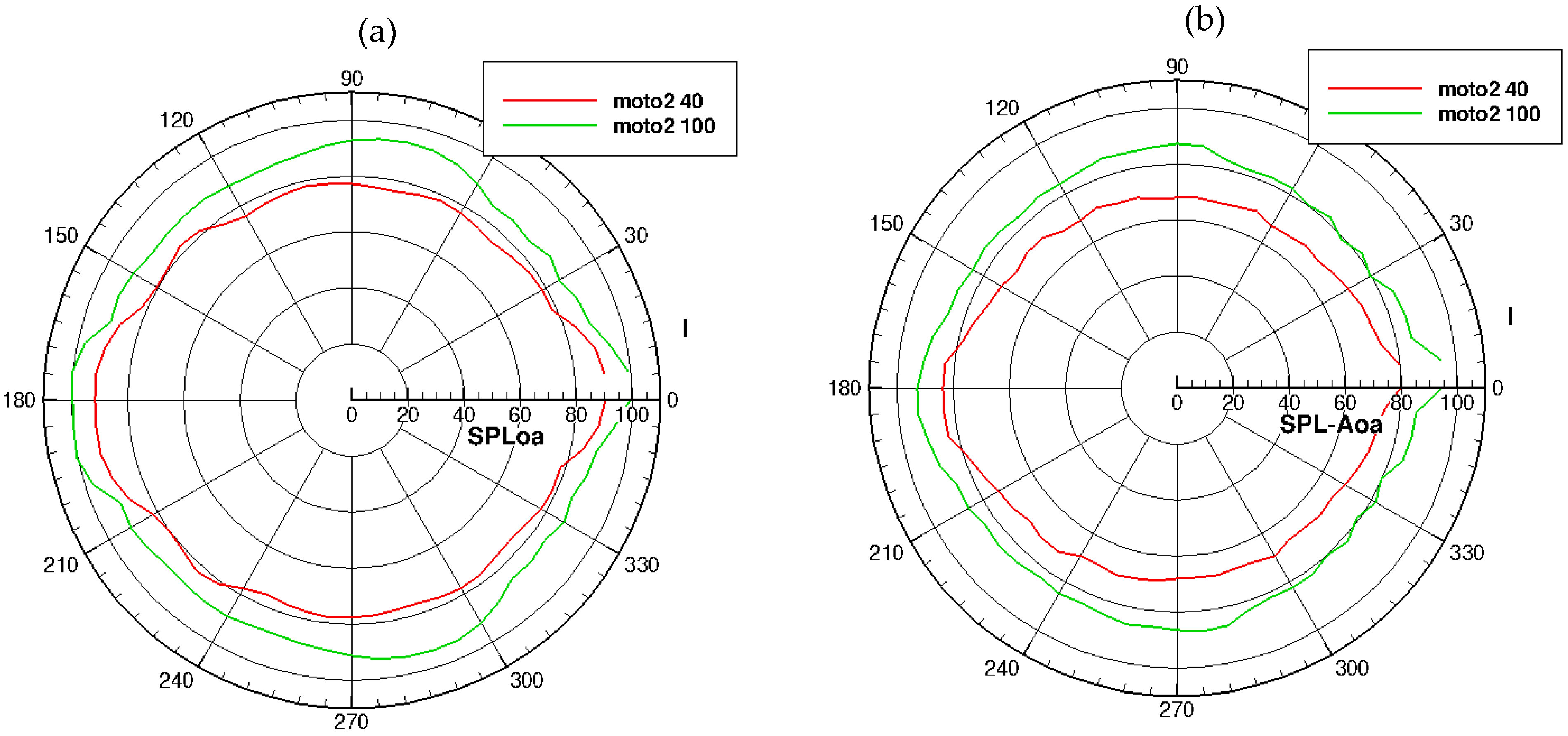
4.2.2. Motorization 2

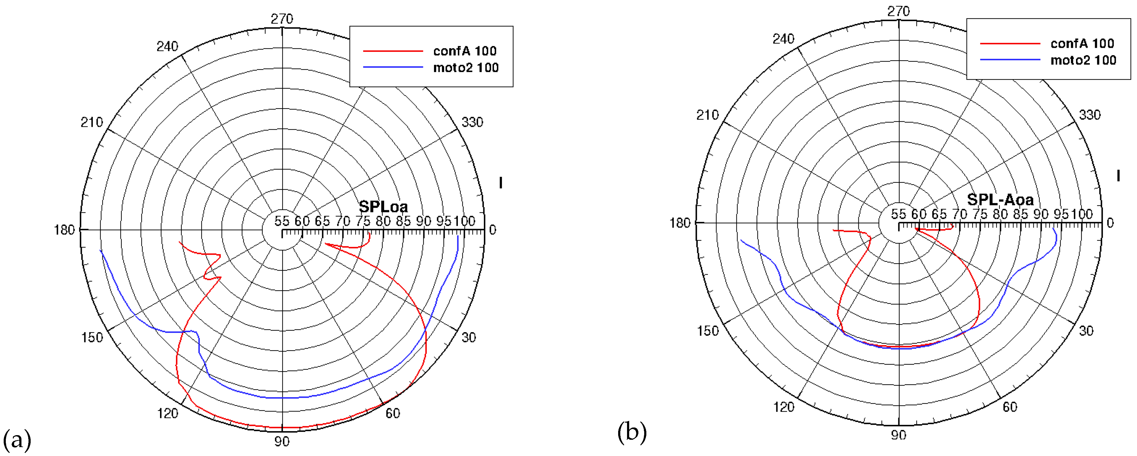
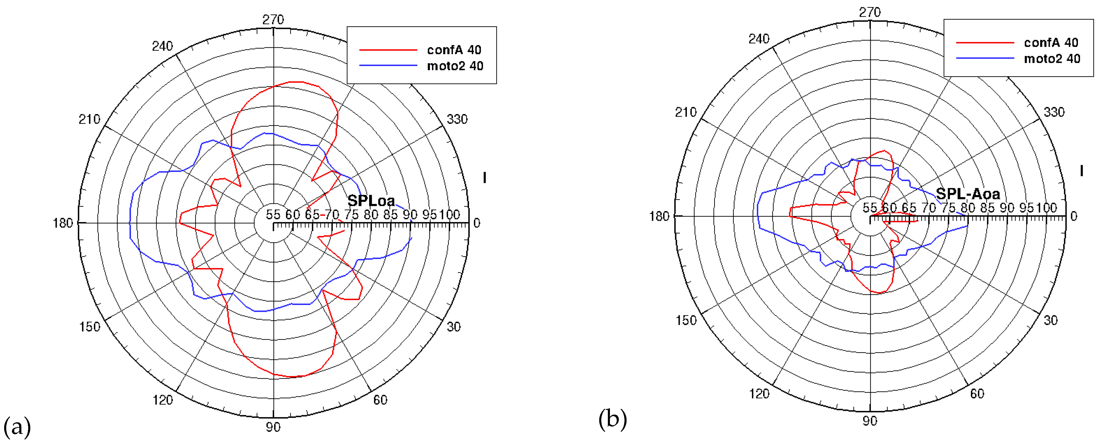
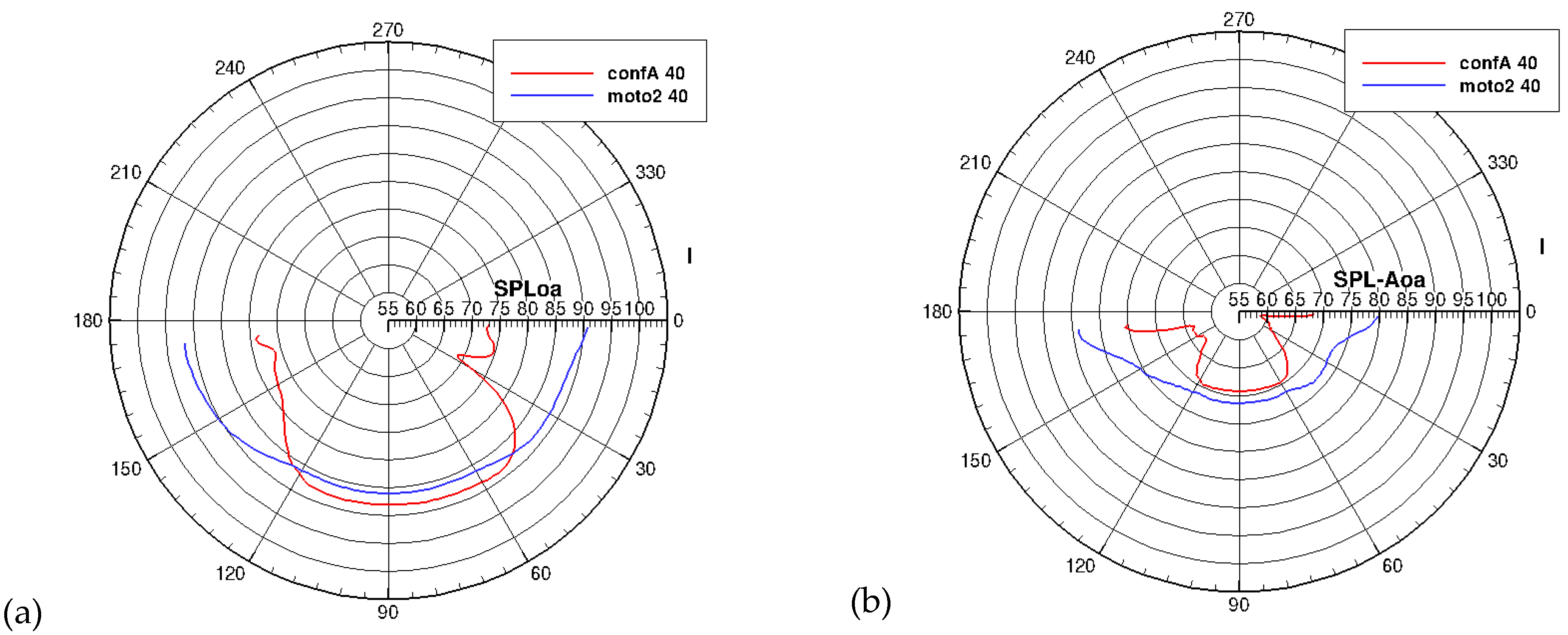
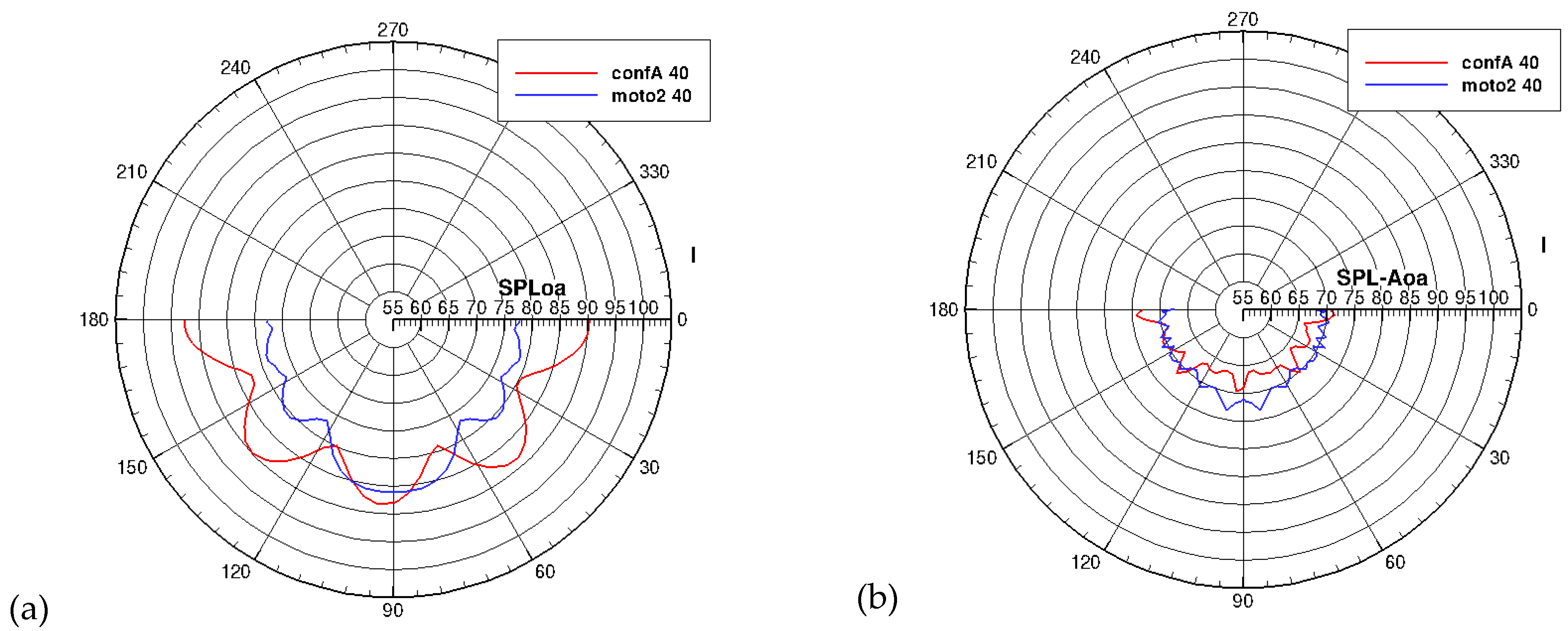
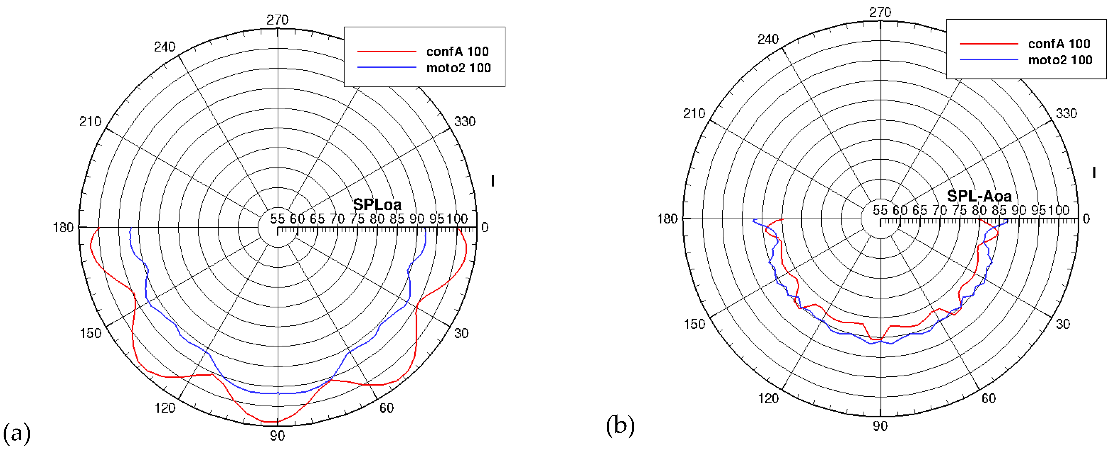
In Figure 21 and Figure 22, the same analyses used in the previous configuration were repeated for the Motorization 2 aircraft. The noise field on the sphere of radius 100 m showed the same behavior as Configuration A. The OASPL field had a different shape, with lower levels of noise in the zones of the propellers, and higher values in the middle, where the fuselage is located, as compared with Configuration A. Similar results are shown in the plot of OASPL-A.

This effect could be related to the tip propellers having low thrust values with respect to the two main propellers in Configuration A, and consequently they contributed less to the overall noise.

Following the methods used in the previous configuration, Figure 23 reports the directivity diagrams in the horizontal XY plane, centered on the position of the aircraft. The noise field is quite similar for both thrust conditions, with greater values for the full thrust configuration.

4.2.3. Comparison

To highlight the differences between the two aircraft configurations, we reported the directivity plot extracted from the sphere in the three main planes. Referring to one of the 3D views of the aeroacoustics sphere, the planes considered are the following: the XY horizontal plane, centered on the position of the aircraft, the XZ longitudinal plane, extending from the front to the rear of the aircraft, and the YZ transverse plane, extending from the left to the right of the aircraft.

In Figure 24 and Figure 25, the comparison of the OASPL and OASPL-A values in the XY horizontal plane, for both 40% and 100% thrust levels, shows that the noise filed is greater in the X direction (0–180 degrees) for the Motorization 2 configuration than in Configuration A, while in the lateral Y direction (90–270 degrees), there was an opposite behavior. This noise pattern is confirmed, in Figure 26 and Figure 27, for the longitudinal direction, where the noise field of Motorization 2 is more extended than in the other configuration. In particular, in the zone just under the axis origin (where is located the aircraft), the noise level of Configuration A aircraft is greater than Motorization 2. It is worth noting that in the A-weighted scale this effect disappears because the higher frequencies of the distributed propellers have greater contributions to overall noise levels. In Figure 28 and Figure 29, the results highlighted in the previous figures are also proved in the transverse direction. The classical Configuration A showed greater noise level on the SPL scale than did Motorization 2, while in the SPL A-weighted scale, the opposite situation was proven.

The propellers in the baseline configuration have a quasi-perfect dipole behaviour, characterized by an acoustic directivity with a maximum around the propellers disk and the minimum around the propellers’ axes, as highlighted in Figure 18 and Figure 27. Conversely, the DEP configuration exhibits a more complex directivity due to the DEP-wing aerodynamic interactions, as shown in Figure 21, providing higher noise values in the longitudinal direction (in front of and behind the aircraft).

In

Table 6. Average SPL values.

	SPL Average [dB]	SPL-A Average [dB]
Configuration A, 40% ETR	85.117	66.967
Motorization 2, 40% ETR	84.269	72.189
Configuration A, 100% ETR	98.675	80.036
Motorization 2, 100% ETR	93.759	85.197

, the overall sound pressure levels averaged for the two configurations are reported. In term of SPL, the classical Configuration A had greater noise values compared with the hybrid configuration, as was expected from the hemispheric noise field comparison. In term of the A-weighted scale, where the contribution of higher frequencies is more relevant, the hybrid configuration Motorization 2 had higher noise levels due to the higher BPFs of the distributed propellers.

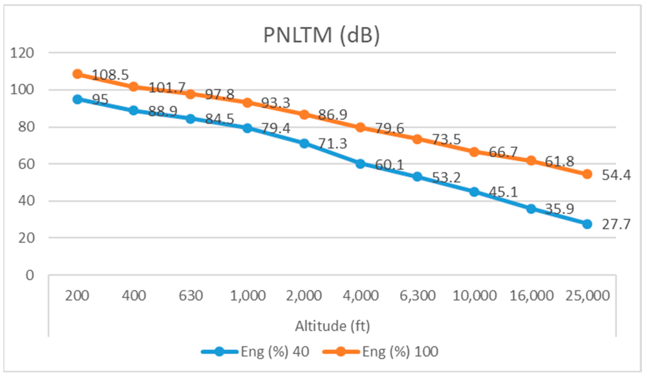
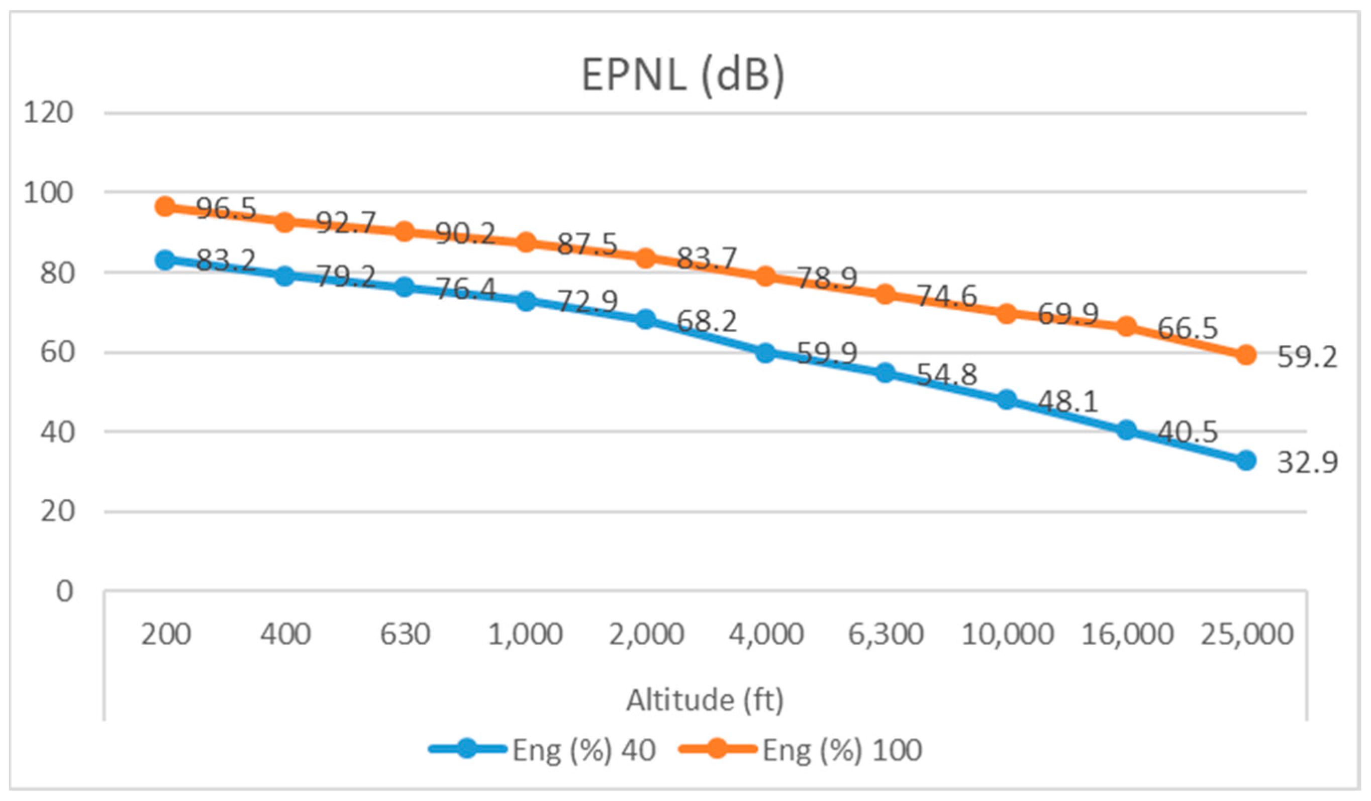
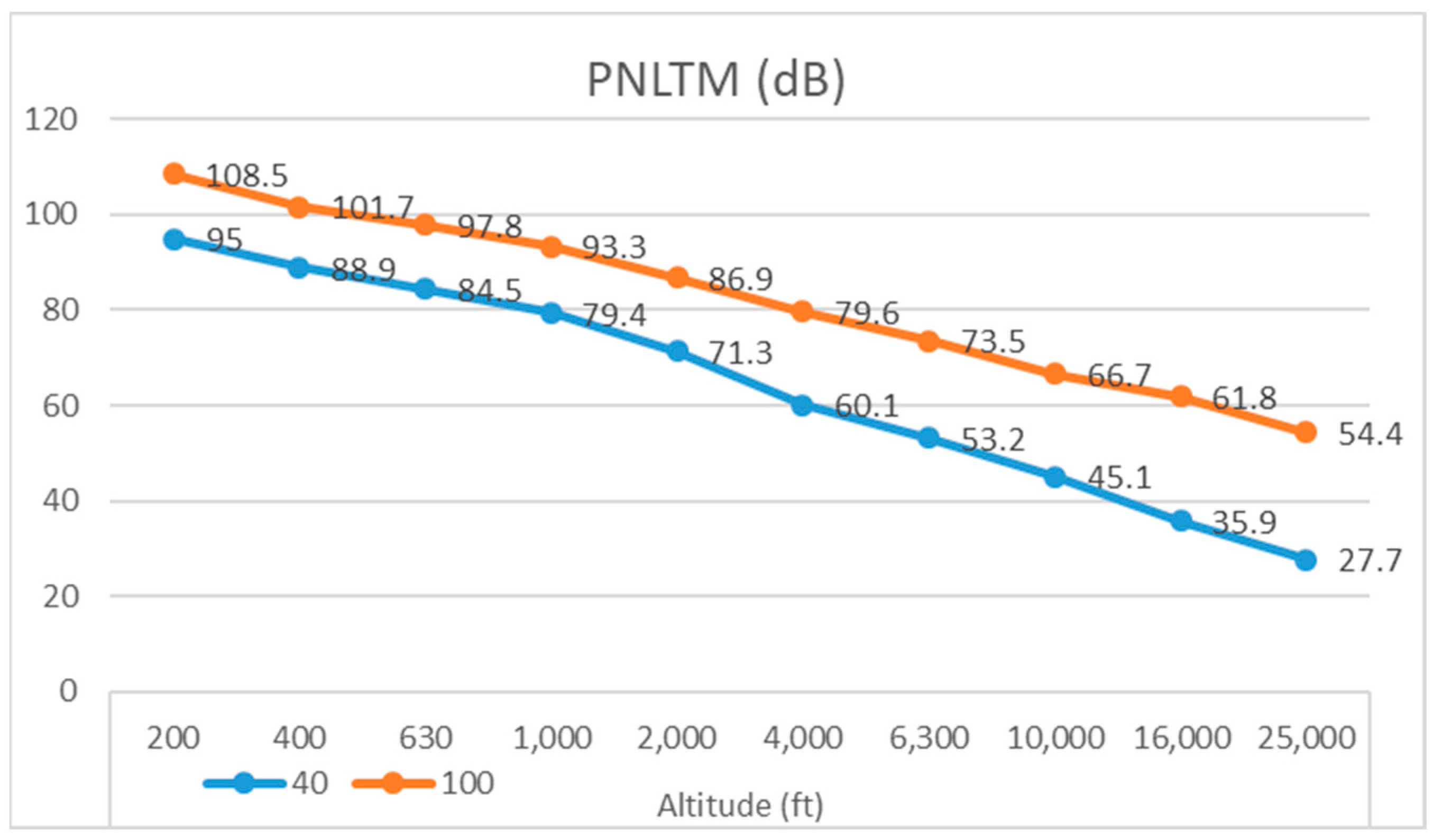
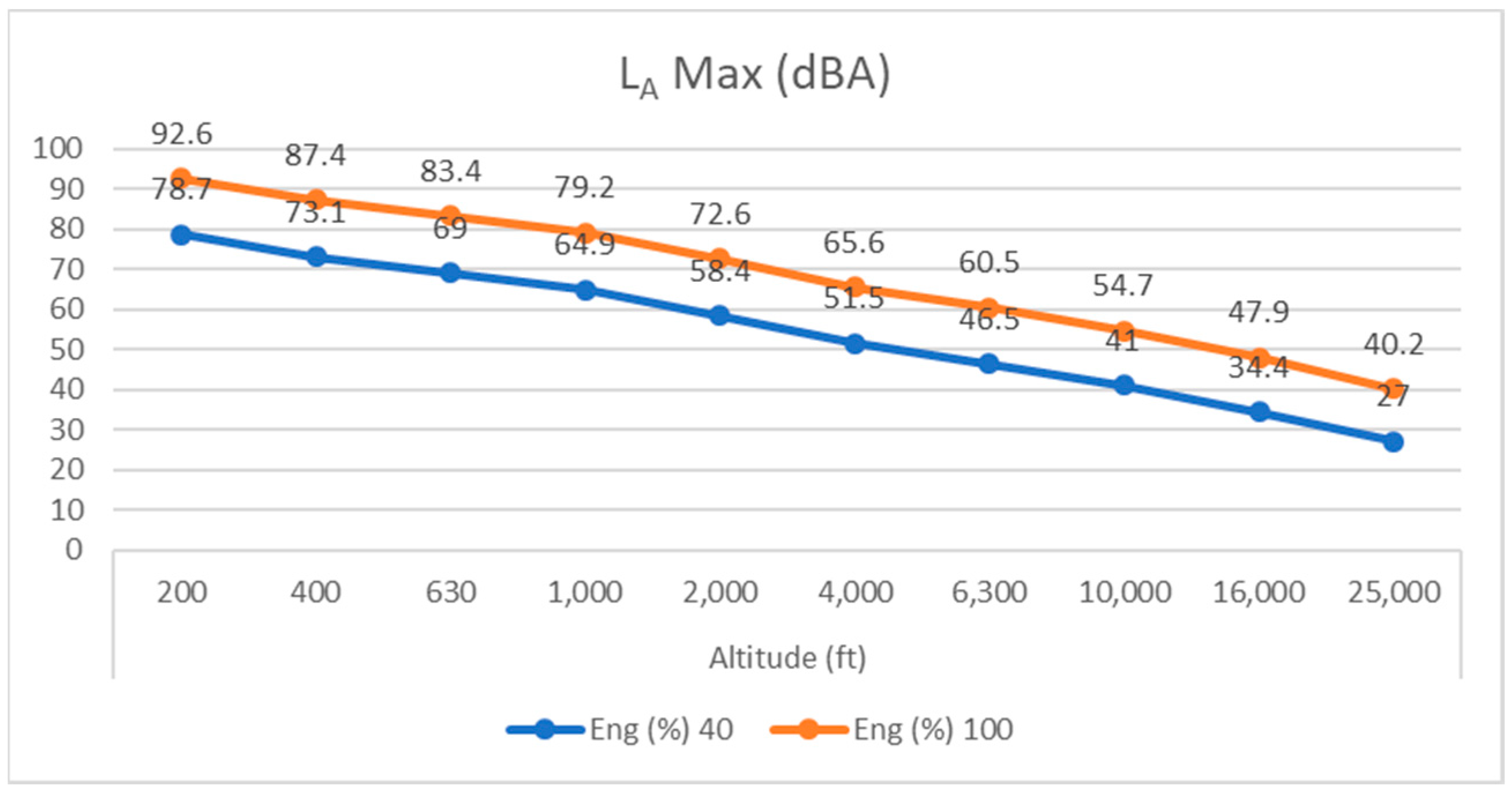
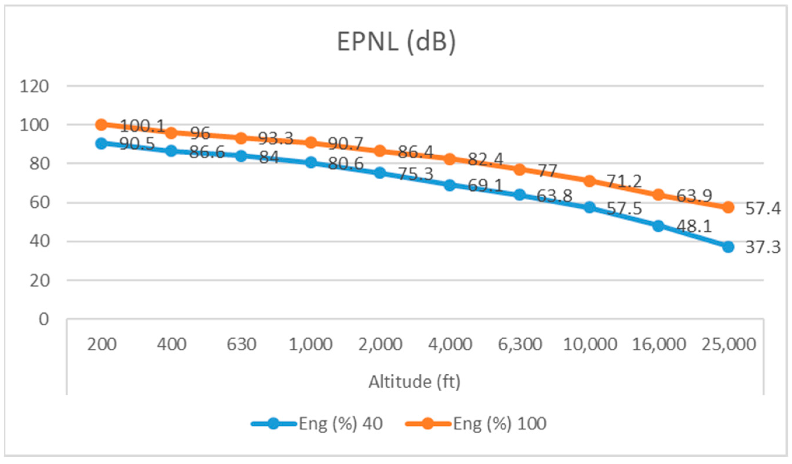
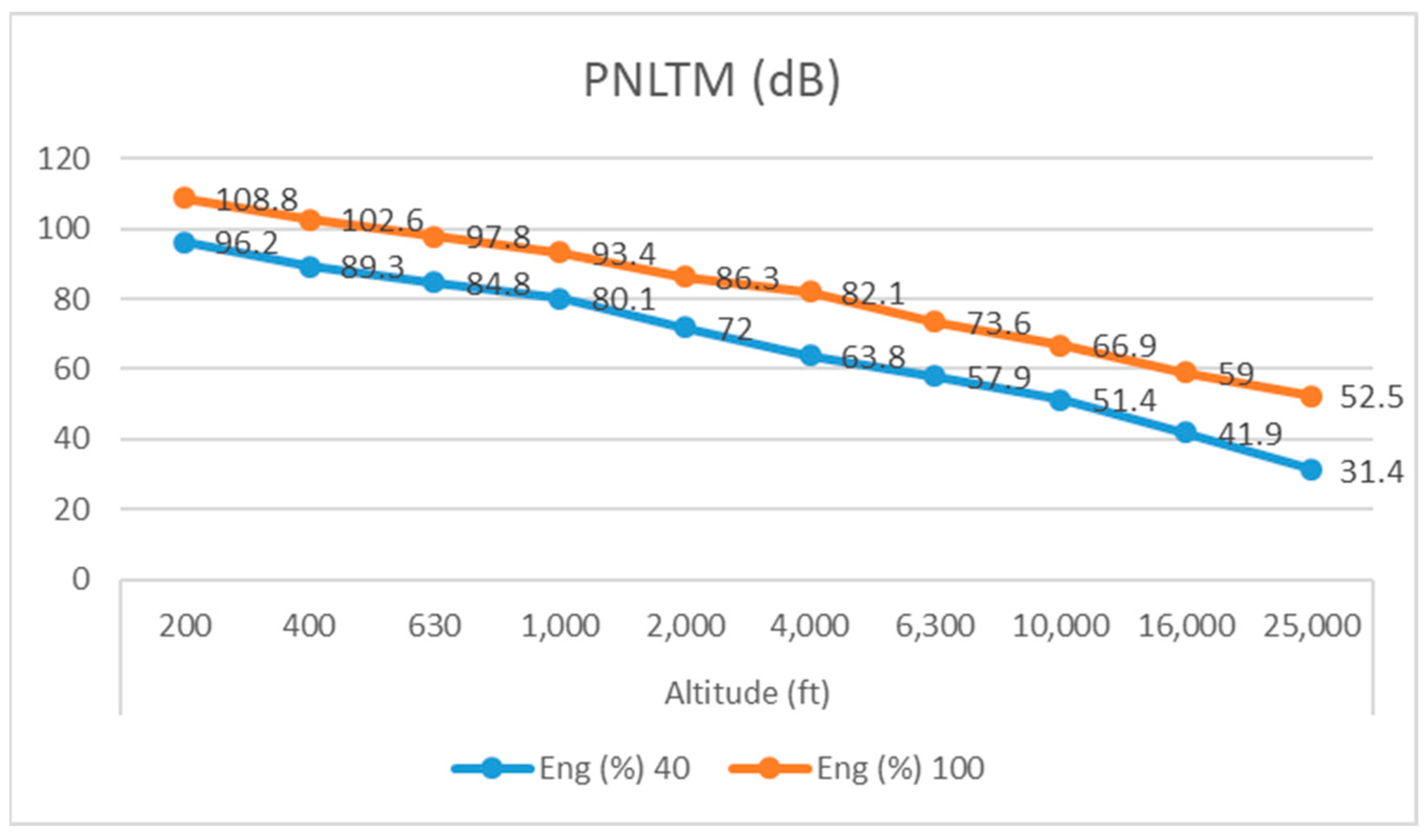
4.3. The NPD Database Generation

In this section, the NPD database is reported for each of the configurations of the vehicle here considered.

By adopting the numerical process described in the previous section, acoustic databases of noise–power–distance were built. The considered engine power setting for the two configurations of the aircraft, were 40% and 100%, while the altitude was set as per the requirements of the AEDT software, starting at 200 ft and ending at 25,000 ft. It is worth noting that 200 ft is 60.96 m; while the radius of hemisphere for the acoustic source modelling is longer (100 m) than this altitude, validity problems may occur while performing the numerical simulations at this altitude. Indeed, the simulation finds a distance between the source and microphone less than 100 m, and so performs a non-valid calculation of the real acoustic effect on the observation point. For this reason, the data obtained for 200 ft altitude are shown but considered merely an appraisal of reliable data.

Figure 30, Figure 31, Figure 32 and Figure 33 report the NPD database for the ATR aircraft configuration, respectively in terms of sound exposure level (L_AE), the peak value of the A-weighted instantaneous sound level (L_AMax), the effective perceived noise level (EPNL), and the maximum value of the perceived noise level with tone correction (PNLTM).

Figure 34, Figure 35, Figure 36 and Figure 37 report the NPD database for the DEP aircraft configuration, with the same variables as in the ATR configuration.

The results show the DEP configuration was significantly louder than the ATR one. The higher the altitude, the lower the difference between the two configurations; this is related to the atmospheric absorption and the characteristic spectral contents of the two sources. Concerning the greater loudness of the DEP configuration, Figure 38 compares the A-weighted instantaneous sound levels (L_A) for the two configurations at 40% engine power and an altitude of 400 ft. The solid red line represents the time variation of L_A for the DEP configuration along the numerical simulation of the acoustic experiment, while the blue solid line is the same for the ATR configuration. It is evident that the DEP configuration always had greater sound levels, mainly due the acoustic effect of the mid-wing propellers (perfectly equal and reported as dash-dotted green lines), while the two wingtip propellers (perfectly equal and reported as dash-dotted black lines) had negligible acoustic contributions.

4.4. Airport Acoustic Impact Assessment

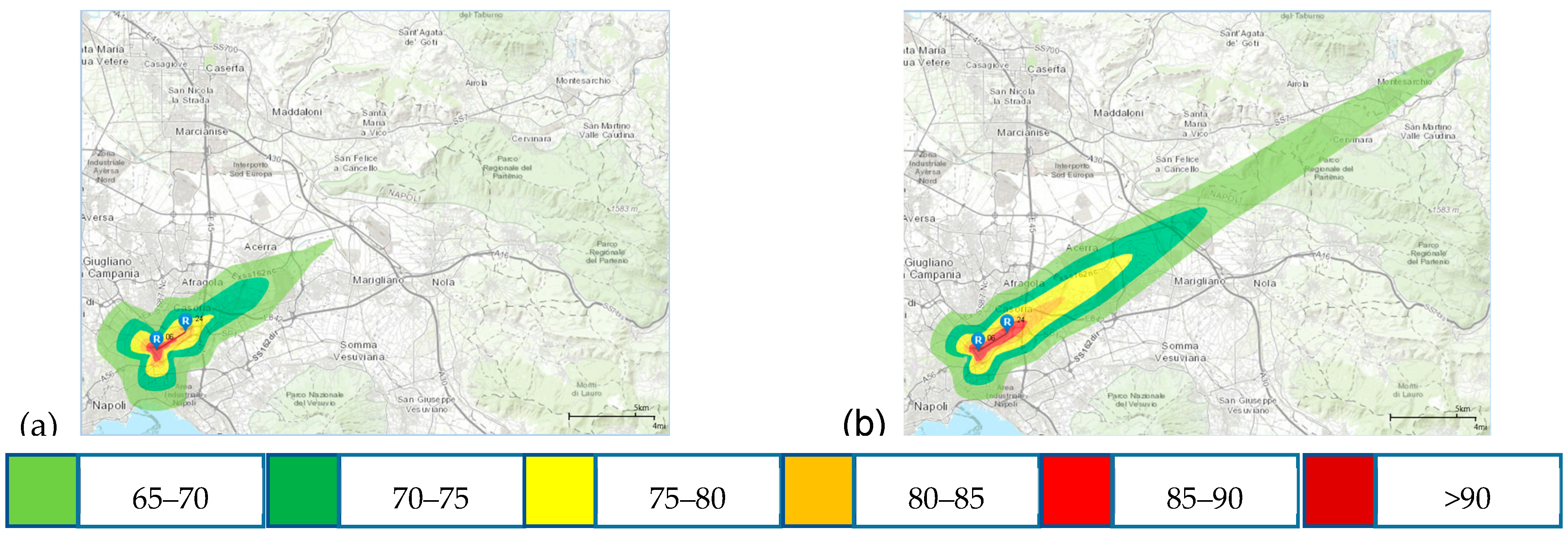
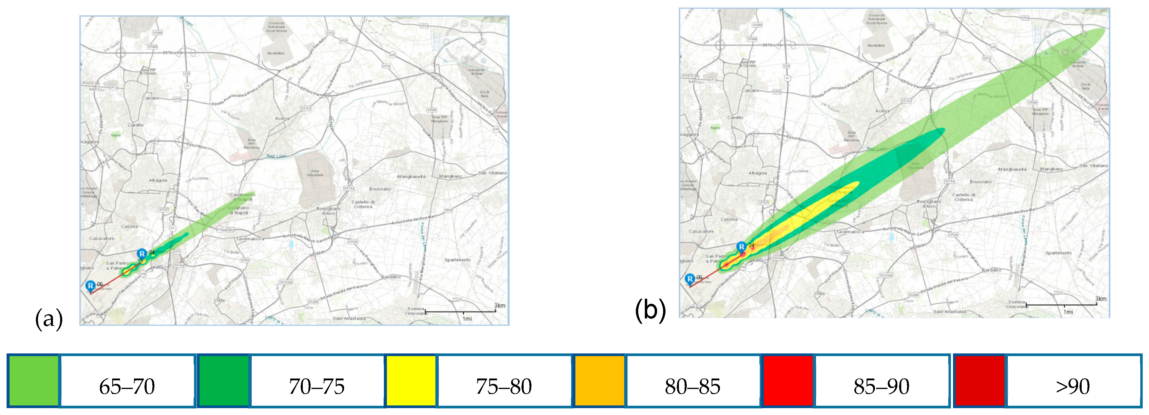
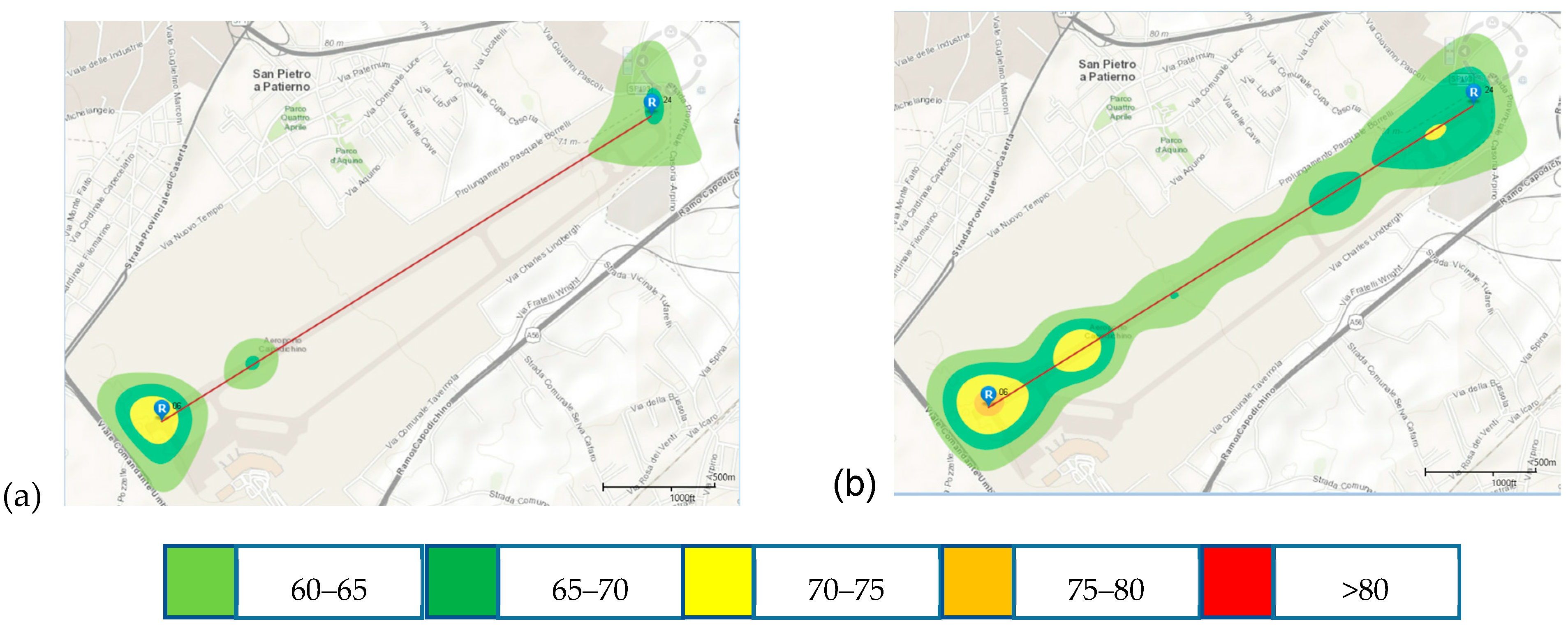
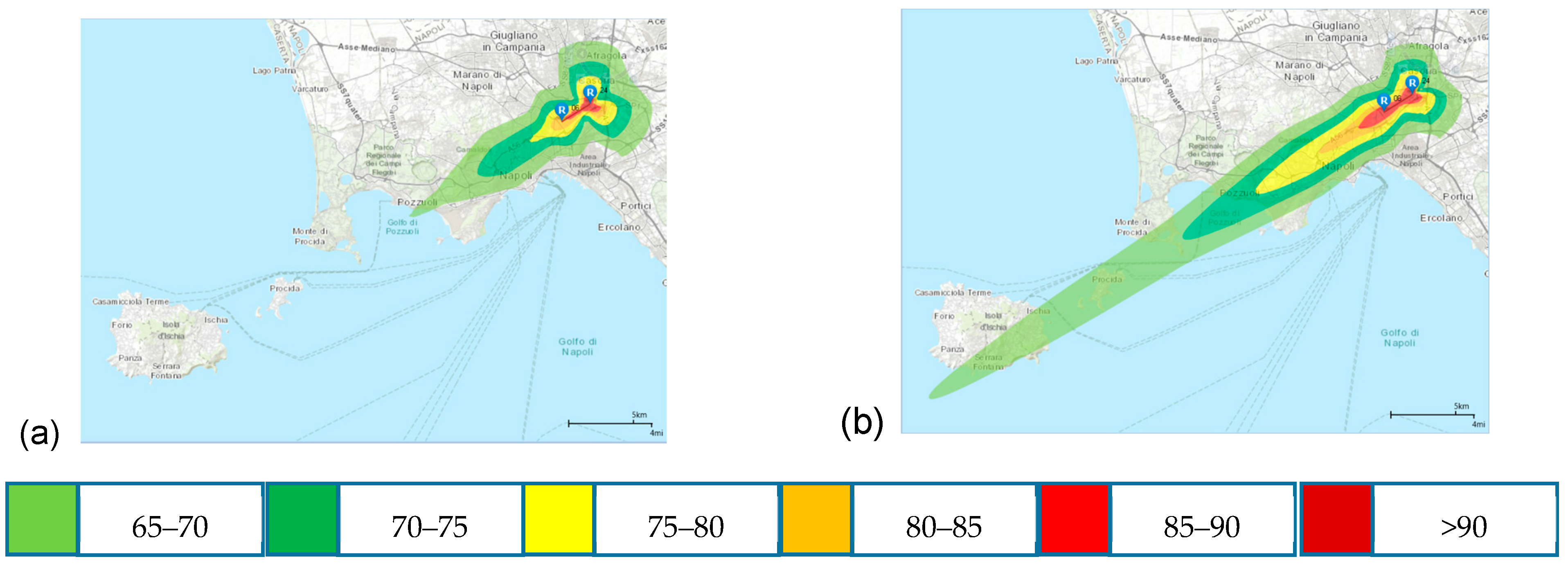
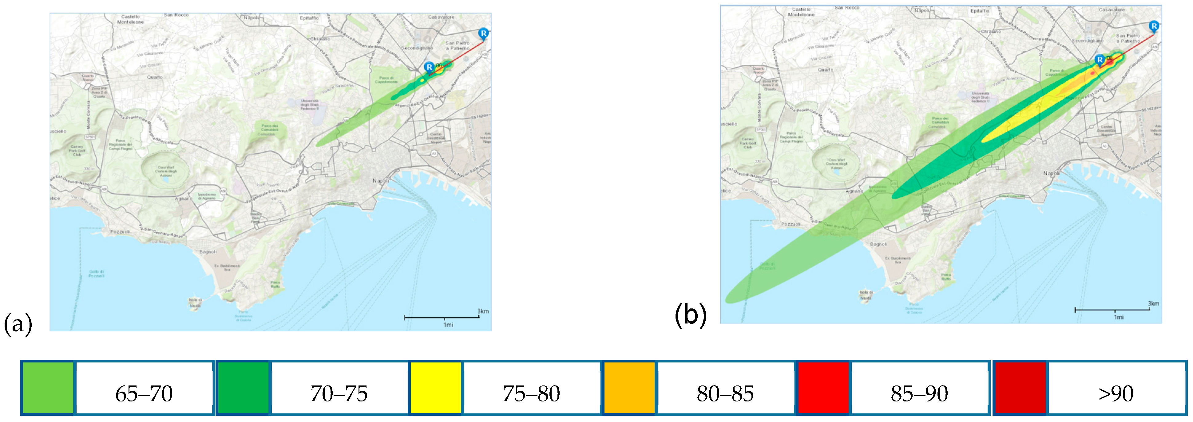
4.4.1. Capodichino Airport: Single Operations

This section describes the noise impact prediction model relative to Capodichino airport for both the ATR42-500 conventional aircraft (configuration A) and the hybrid motorization (version 2.2), by using the previously calculated NPD curves and the procedural flight profiles present in the AEDT database, modified with the data in [22].

Figure 39, Figure 40, Figure 41 and Figure 42 show noise area extensions and the disturbed population for ATR42 during standard take-off and landing operations at Capodichino airport, in terms of L_AE, for conventional and hybrid aircraft, on runways 06 and 24.

4.4.2. Capodichino Airport: Cumulative Operations

As requested by the 2005 Decree n. 194, the acoustic mapping of Naples Capodichino Airport, relative to ATR42 aircraft, by using the acoustic descriptors defined in the same decree, were carried out. We assumed an annual traffic scenario of 4200 take-offs and 4200 landings, equally distributed between the two runway heads. The majority (90%) of operations were concentrated in the day period (from 06.00 to 20.00), while the remaining 10% were in the evening period (from 20.00 to 22.00) (see

Table 7. ATR42-500 annual traffic scenario.

	Rw	Nr operations Day (6–20)	Nr Operations Evening (20–22)	Total Nr. of Operations
Take-off	24	3780	420	4200
Landing	24	3780	420	4200
Take-off	06	3780	420	4200
Landing	06	3780	420	4200

).

In Figure 43, noise contour surfaces, expressed in geo-localized L_DEN, are illustrated for the conventional and hybrid configurations. Observing the graphic representation, we can appreciate the extension of its contours and the invested territorial areas.

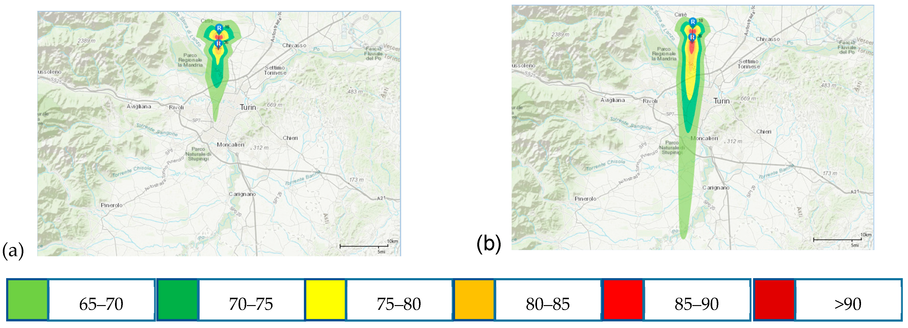
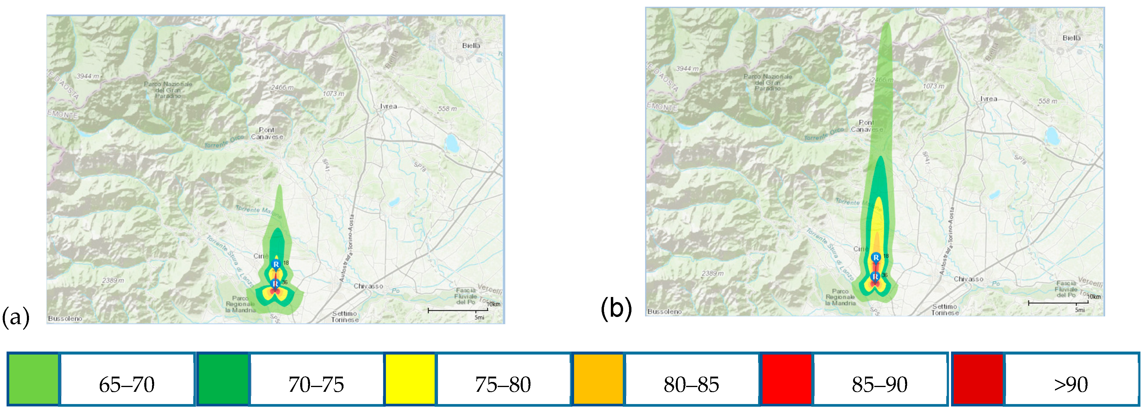
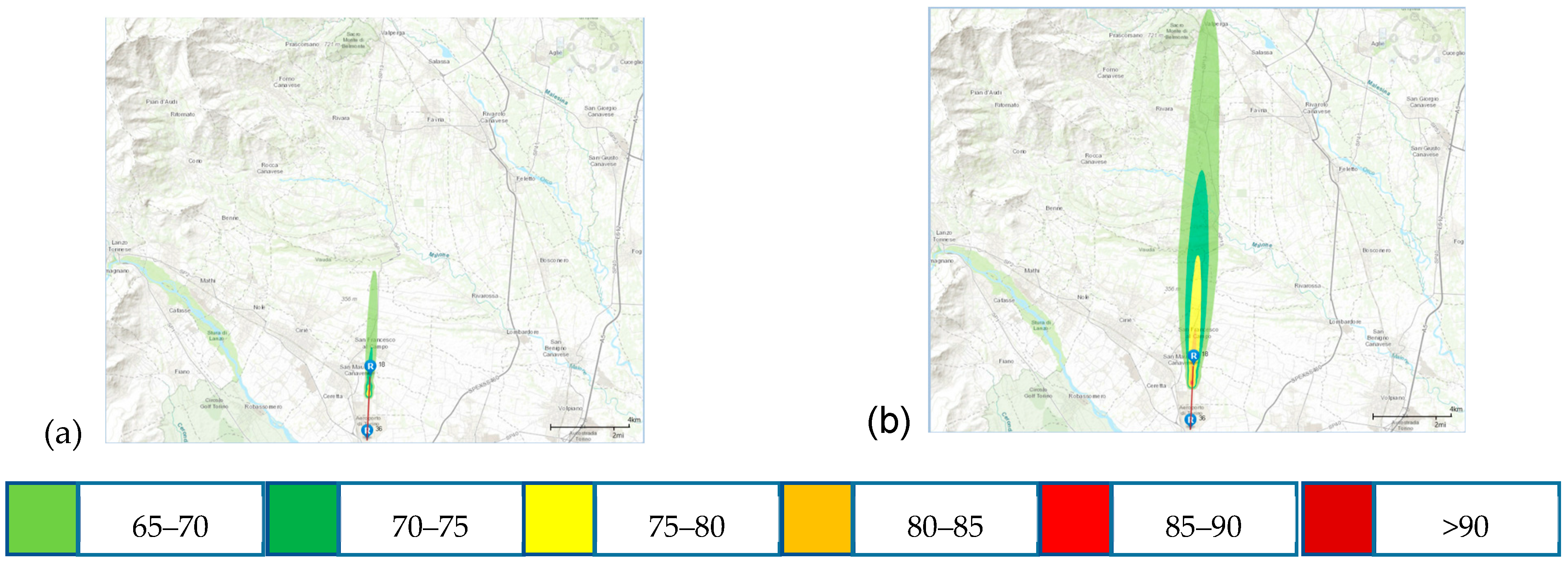
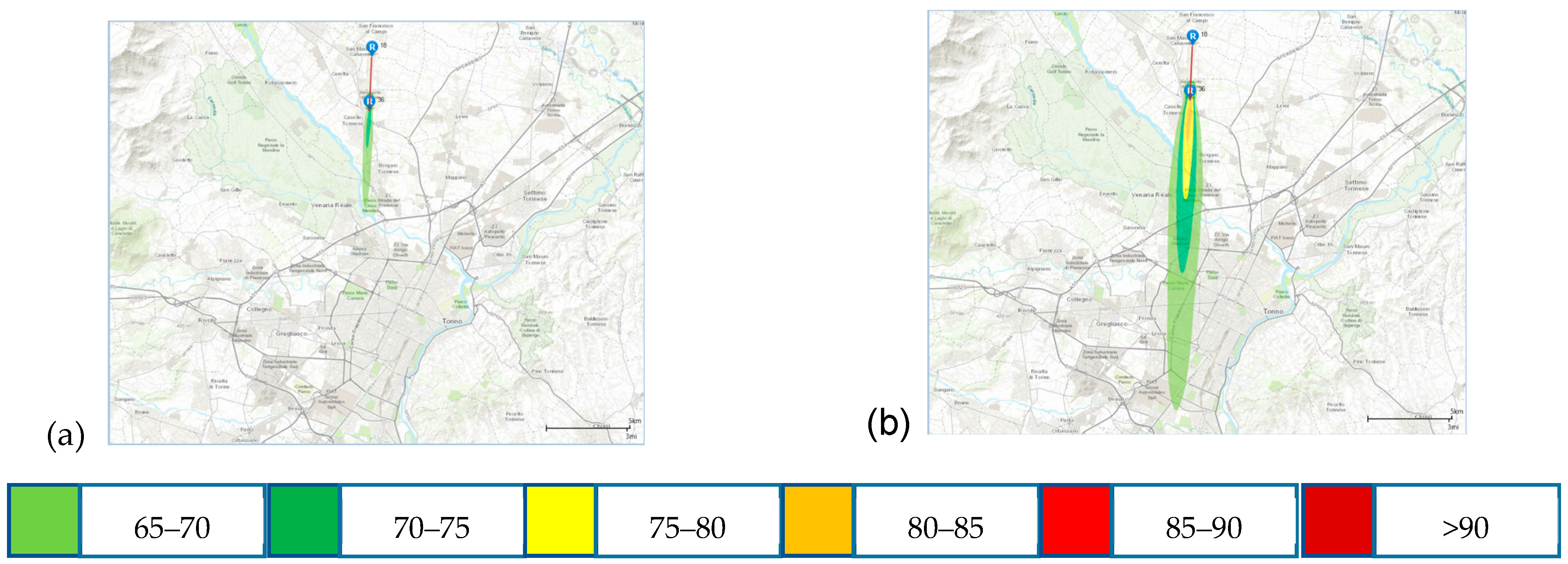
4.4.3. Turin Airport: Single Operations

The noise impact prediction model, relative to Caselle airport, for both ATR42-500 conventional aircraft (configuration A) and hybrid motorization (version 2.2), by using the NPD curves calculate in previous paragraph and the procedural flight profiles present in the AEDT database modified with the data in [22], are next discussed.

Figure 44, Figure 45, Figure 46 and Figure 47 depict the extensions of the noise area of population disturbance for ATR42 during standard take-off and landing operations at Turin airport, in terms of L_AE, for conventional and hybrid aircraft on runways 18 and 36.

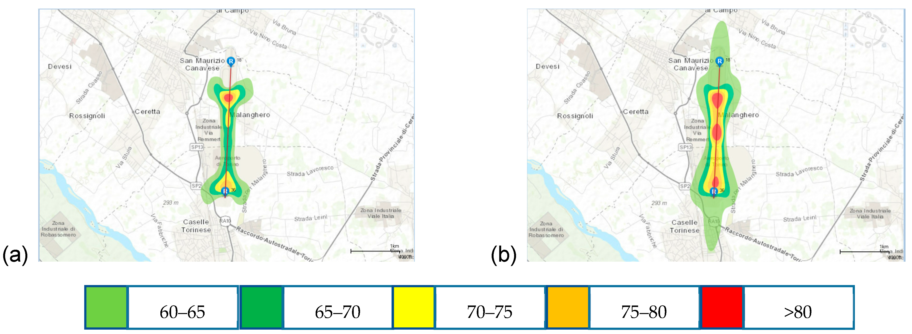
4.4.4. Turin Airport: Cumulative Operations

As requested by the 2005 Decree n. 194, the acoustic mapping of Turin Caselle Airport for ATR42 aircraft, by using the acoustic descriptors defined in the same decree, was carried out. We assumed an annual traffic scenario of 4200 take-offs and 4200 landings, equally distributed between the two runway heads. The majority (90%) of operations were concentrated in the day period (from 06.00 to 20.00), while the remaining 10% were concentrated in the evening period (from 20.00 to 22.00) (see

Table 8. ATR42-500 annual traffic scenario.

	Rw	Nr Operations Day (6–20)	Nr Operations Evening (20–22)	Total Nr. of Operations
Take-off	18	3780	420	4200
Landing	18	3780	420	4200
Take-off	36	3780	420	4200
Landing	36	3780	420	4200

).

Figure 48 shows extensions of the noise area of population disturbance for ATR42 annual operations, in terms of L_DEN, for conventional and hybrid aircraft.

4.4.5. Comparison of Results

The acoustic impact on airport runways shown above are strictly related to the NPD databases provided, which are also the source terms for the AEDT method. Considering Figure 38, the noise level of the DEP configuration (red line) is wider than that of the baseline configuration (blue line), mainly due to the contribution of the inner-wing DEP propellers (green line). The noise impact on the airport is basically the integral of those curves along the assessed trajectories during the whole observation period; therefore, the resulting subsequent noise values and size of the covered area of the DEP configuration is higher than those of the baseline.

5. Conclusions

Acoustic impact assessments that include new propulsion technologies and new configurations of a regional aircraft (ATR42 pax) in a reference airport area were analysed and are here described.

Two configurations, based on the ATR42 regional aircraft, were investigated:

• Configuration A: the baseline configuration consists of a simplified version of the ATR42 regional aircraft equipped with two thermal engines, located in the proximity to the fuselage;
• Motorization 2: the hybrid-electric configuration consists of a modified version of the ATR42 regional aircraft with a new wing of equal length and higher aspect ratio, two tip propellers powered by thermal engines, aiming at reducing the induced drag, and a DEP system comprised of four propellers per side, powered by electric motors.

An evaluation of the noise impact from tonal components was made by characterizing the aircraft as a noise source and then assessing the impacts of its operation. To this end, a procedure was set up at CIRA consisting of the following main steps:

• The evaluation of the aerodynamic pressures on the full configuration via a medium-fidelity aerodynamic solver;
• The evaluation of aeroacoustic performance and a hemispheric noise field, using the FW–H approach;
• The generation of noise–power–distance (NPD) databases by a ray-tracing approach;
• The evaluation of the acoustic impacts at the airport level by AEDT procedure.

The aerodynamic results highlighted the strong interactional process between the propellers, their wakes, and the aircraft, which was considerably higher in the DEP configuration because of the many propellers installed. In particular, a stronger impact was observed at the leading edge of the wing where an increased pressure expansion was generated in the region impinged by the propellers’ wakes. This effect was especially significant for the DEP configuration, wherein pressure expansion was observed throughout the wing span, and in between the two innermost propellers, where the expansion extended to more than half the wing chord.

The aeroacoustics analyses show the differences in the tonal noise fields generated by the two configurations. The baseline Configuration A showed a lower noise impact in the longitudinal direction than the hybrid-electric Motorization 2 aircraft, while in the lateral direction, an opposite behavior was observed. This effect is due to the different thrust distributions among the tip and DEP propellers in the hybrid configuration, as compared with the two main propellers of the baseline configuration. Comparing the two configurations in term of averaged overall noise, Configuration A had, still, greater noise levels than source levels on the SPL scale, while in term of the A-weighted scale, where the contribution of higher frequencies is more relevant, the hybrid configuration, Motorization 2, was noisier due to the higher BPFs of the distributed propellers.

To model the aircraft noise impact analysis, airports from Naples and Turin as references, the above mentioned two configurations based on the ATR42 regional aircraft, the FAA AEDT software and noise–power–distance (NPD) as generated by RALPH code were used. Notably, standard take-off and landing profiles have been considered.

For both configurations, single and cumulative operations were analyzed, and their impacts on the population were assessed.

By comparing the results relatively between the two configurations under examination, it appears clear that the tonal contribution of the hybrid configuration had a much greater impact than that of the baseline, both in terms of the areas touched and the populations involved at both airports under study.

References

1. PROSIB—Capitolato Tecnico ARS01_00297. Propulsione E Sistemi Ibridi per Velivoli ad Ala Fissa E Rotante; Ministero dell’Istruzione, dell’Università e della Ricerca: Rome, Italy, 2018. [Google Scholar]
2. Aversano, R.; Bianco, D.; De Vivo, L.; Sollazzo, A.; Barbarino, M.; Federico, L. Acoustical Characterization of the F-35A Joint Strike Fighter: Results and Perspectives of the First Experimental Campaign; Institute of Noise Control Engineering: Madrid, Spain; ISBN 978-84-87985-31-7. ISSN 0195-175x. Available online: http://www.sea-acustica.es/fileadmin/INTERNOISE_2019/Fchrs/Proceedings/2003.pdf (accessed on 11 January 2021).
3. SAE. Procedure for the Calculation of Airplane Noise in the Vicinity of Airports; SAE AIR 1845A; SAE International: Warrendale, PA, USA, 2012. [Google Scholar] [CrossRef]
4. ICAO Annex 16 Vol. 1 “Aircraft Noise”. Available online: https://store.icao.int/en/annex-16-environmental-protection-volume-i-aircraft-noise (accessed on 11 January 2021).
5. Visingardi, A.; D’Alascio, A.; Pagano, A.; Renzoni, P. Validation of CIRA’s Rotorcraft Aerodynamic Modelling SYStem with DNW Experimental Data. In Proceedings of the 22nd European Rotorcraft Forum, Brighton, UK; 1996. Available online: https://dspace-erf.nlr.nl/xmlui/handle/20.500.11881/3171 (accessed on 13 January 2021).
6. Visingardi, A.; Dummel, A.; Falchero, D.; Pidd, M.; Voutsinas, S.G.; Yin, J. Aerodynamic interference in full helicopter configurations: Validation using the HeliNOVI database. In Proceedings of the 32nd European Rotorcraft Forum, Maastricht, The Netherlands, 12–14 September 2006; Available online: http://hdl.handle.net/20.500.11881/1080 (accessed on 13 January 2021).
7. De Gregorio, F.; Visingardi, A.; Iuso, G. An Experimental-Numerical Investigation of the Wake Structure of a Hovering Rotor by PIV Combined with a G2 Vortex Detection Criterion. Energies 2021, 14, 2613. [Google Scholar] [CrossRef]
8. Casalino, D.; Genito, M.; Visingardi, A. Numerical Analysis of Airframe Noise Scattering Effects in Tilt Rotor Systems. AIAA J. 2007, 4, 45. [Google Scholar] [CrossRef]
9. Morino, L. A General Theory of Unsteady Compressible Potential Aerodynamics. NASA CR-2464. 1974. Available online: https://ntrs.nasa.gov/citations/19750004821 (accessed on 13 January 2021).
10. Casalino, D. An advanced time approach for acoustic analogy predictions. J. Sound Vib. 2003, 4, 583–612. [Google Scholar] [CrossRef]
11. Pagano, A.; Barbarino, M.; Casalino, D.; Federico, L. Tonal and Broadband Noise Calculations for Aeroacoustic Optimization of a Pusher Propeller. AIAA J. Aircr. 2010, 3, 47. [Google Scholar] [CrossRef]
12. Casalino, D.; Barbarino, M.; Visingardi, A. Simulation of Helicopter Community Noise in Complex Urban Geometry. AIAA J. 2011, 49, 1614–1624. [Google Scholar] [CrossRef]
13. Barbarino, M.; Petrosino, F.; Visingardi, A. A High-Fidelity Aeroacoustic Simulation of a VTOL Aircraft in an Urban Air Mobility Scenario. Aerosp. Sci. Technol. 2021, 107104, 1270–9638. [Google Scholar] [CrossRef]
14. UNI-ISO 9613-2:2006. Acoustics—Attenuation of Sound During Propagation Outdoors—Part 2: General Method of Calculation. Available online: http://store.uni.com/catalogo/norme/root-categorie-ics/17/17-140/17-140-01/uni-iso-9613-2-2006 (accessed on 13 January 2021).
15. ICAO. Doc 9501. Environmental Technical Manual: Volume I—Procedures for the Noise Certification of Aircraft. Available online: https://store.icao.int/en/environmental-technical-manual-volume-1-procedures-for-the-noise-certification-of-aircraft-doc-9501-1 (accessed on 18 January 2021).
16. SAE. Standard Values of Atmospheric Absorption as a Function of Temperature and Humidity; SAE ARP866B; SAE International: Warrendale, PA, USA, 1975. [Google Scholar] [CrossRef]
17. De Vivo, L. Model for Aircraft Noise Impact Analysis in a Reference Airport, PROSIB Project, Deliverable D3.3.2. December 2020. [Google Scholar]
18. Legge 26 Ottobre 1995, n. 447 “Legge Quadro sull’Inquinamento Acustico”. Available online: https://www.gazzettaufficiale.it/eli/id/1995/10/30/095G0477/sg (accessed on 18 January 2021).
19. Decreto Ministeriale 31 Ottobre 1997 “Metodologia di Misura del Rumore Aeroportuale”. Available online: https://www.gazzettaufficiale.it/eli/id/1997/11/15/097A9090/sg (accessed on 18 January 2021).
20. Decreto Legislativo 194/2005 “Attuazione Della Direttiva 2002/49/CE Relativa Alla Determinazione e Alla Gestione del Rumore Ambientale”. Available online: https://www.gazzettaufficiale.it/eli/id/2005/10/13/05A09688/sg (accessed on 18 January 2021).
21. Crocker, M.J. Handbook of Noise and Vibration Control; John Wiley & Sons: Hoboken, NJ, USA, 2007; p. 15. ISBN 978-0-471-39599-7. [Google Scholar]
22. University of Napoli, Leonardo Divisione Velivoli, PROSIB D2.1.5—Progetto preliminare e MDO velivolo motorizzazione 2, PROSIB project. September 2020.
23. Pagano, A. Progetto e Verifica Elica per Velivoli con Ala Convenzionale della Classe ATR42-Ottimizzazione Elica—Design and Verification of Propellers for Conventional Wings of the ATR42 Aircraft Class—Propeller Optimization (in Italian), PROSIB project, deliverable D2.1.2. December 2019. [Google Scholar]
Figure 1. The process of the NPD database calculation.
Applsci 11 09664 g001
Figure 2. Capodichino Airport (source: www.aeroportodinapoli.it, accessed on 1 March 2021).
Applsci 11 09664 g002
Figure 3. Turin-Caselle Airport (source: www.aeroportoditorino.it accessed on 1 March 2021).
Applsci 11 09664 g003
Figure 4. Configuration A.
Applsci 11 09664 g004
Figure 5. Motorization 2.
Applsci 11 09664 g005
Figure 6. Rotor blade discretized geometry.
Applsci 11 09664 g006
Figure 7. CAD representation of the airframe.
Applsci 11 09664 g007
Figure 8. Airframe structured-surface meshing.
Applsci 11 09664 g008
Figure 9. Rotor blades’ discretized geometry. Tip propeller (a); DEP propellers (b).
Applsci 11 09664 g009
Figure 10. CAD representation of the airframe.
Applsci 11 09664 g010
Figure 11. Half the span of the airframe structured-surface meshing.
Applsci 11 09664 g011
Figure 12. Configuration A—Cp distribution and wake development in a 100%-ETR climb.
Applsci 11 09664 g012
Figure 13. Configuration A—the thrust (a) and induced-torque (b) time histories in a 100%-ETR climb.
Applsci 11 09664 g013
Figure 14. Configuration A—CN M2 distribution on propellers’ disks. Starboard side (a,c); portside (b,d), in the two cases of Climbing (a,b) and Descent (c,d) flight.
Applsci 11 09664 g014
Figure 15. Motorization 2—Cp distribution and wake development in a 100%-ETR climb, isometric view (a) and view from above the aircraft (b).
Applsci 11 09664 g015
Figure 16. Motorization 2—thrust (a) and induced-torque (b) time histories in a 100%-ETR climb.
Applsci 11 09664 g016
Figure 17. Motorization2—CN M2 distribution on the propellers’ disks, starboard side. From (ae), load on the disk from Tip to inner propellers, in Climb condition. From (fl), same results in Descent flight.
Applsci 11 09664 g017
Figure 18. Configuration A, OASPL, in decibels, on the sphere, top view, in the two flight conditions analysed.
Applsci 11 09664 g018
Figure 19. Configuration A, OASPL-A, in decibels, on the sphere, top view, in the two flight conditions analysed.
Applsci 11 09664 g019
Figure 20. Configuration A, OASPL values on the horizontal XY plane (a), A-weighted values on (b). Comparison between 40% and 100% ETR.
Applsci 11 09664 g020
Figure 21. Motorization 2, OASPL, in decibels, on the sphere, top view, in the two flight conditions analysed.
Applsci 11 09664 g021
Figure 22. Motorization 2, OASPL-A, in decibels, on the sphere, top view, in the two flight conditions analysed.
Applsci 11 09664 g022
Figure 23. Motorization 2, OASPL values on the horizontal XY plane (a), A-weighted values on (b). Comparison between 40% and 100% ETR.
Applsci 11 09664 g023
Figure 24. Comparison between Configuration A and Motorization 2; OASPL values on the horizontal XY plane (a), A-weighted values on (b). Flight condition Descent 40% ETR.
Applsci 11 09664 g024
Figure 25. Comparison between Configuration A and Motorization 2; OASPL values on the horizontal XY plane (a), A-weighted values on (b). Flight condition Climb 100% ETR.
Applsci 11 09664 g025
Figure 26. Comparison between Configuration A and Motorization 2; OASPL values on longitudinal XZ plane (a), A-weighted values on (b). Flight condition Descent 40% ETR.
Applsci 11 09664 g026
Figure 27. Comparison between Configuration A and Motorization 2; OASPL values on longitudinal XZ plane (a), A-weighted values on (b). Flight condition Climb 100% ETR.
Applsci 11 09664 g027
Figure 28. Comparison between Configuration A and Motorization 2; OASPL values on the transverse YZ plane (a), A-weighted values on (b). Flight condition Descent 40% ETR.
Applsci 11 09664 g028
Figure 29. Comparison between Configuration A and Motorization 2; OASPL values on the transverse YZ plane (a), A-weighted values on (b). Flight condition Climb 100% ETR.
Applsci 11 09664 g029
Figure 30. NPD curves, in terms of LAE, for the ATR configuration.
Applsci 11 09664 g030
Figure 31. NPD curves, in terms of LAMax, for the ATR configuration.
Applsci 11 09664 g031
Figure 32. NPD curves, in terms of EPNL, for the ATR configuration.
Applsci 11 09664 g032
Figure 33. NPD curves, in terms of PNLTM, for the ATR configuration.
Applsci 11 09664 g033
Figure 34. NPD curves, in terms of LAE, for the DEP configuration.
Applsci 11 09664 g034
Figure 35. NPD curves, in terms of LAMax, for the DEP configuration.
Applsci 11 09664 g035
Figure 36. NPD curves, in terms of EPNL, for the DEP configuration.
Applsci 11 09664 g036
Figure 37. NPD curves, in terms of PNLTM, for the DEP configuration.
Applsci 11 09664 g037
Figure 38. Comparison of the instantaneous sound levels of the two configurations.
Applsci 11 09664 g038
Figure 39. Graphical representation of equal loudness contours for the conventional (a) and hybrid (b) configurations, in terms of LAE(dB-A), for a standard runway-24 take-off.
Applsci 11 09664 g039
Figure 40. Graphical representation of equal loudness contours for the conventional (a) and hybrid (b) configurations, in terms of LAE (dB-A), for a standard runway-06 take-off.
Applsci 11 09664 g040
Figure 41. Graphical representation of equal loudness contours for the conventional (a) and hybrid (b) configurations, in terms of LAE (dB-A), for a standard runway-24 landing.
Applsci 11 09664 g041
Figure 42. Graphical representation of equal loudness contours for the conventional (a) and hybrid (b) configurations, in terms of LAE (dB-A), for a standard runway-06 landing.
Applsci 11 09664 g042
Figure 43. LDEN (dB-A) of the assessed traffic scenario for the conventional (a) and hybrid (b) configurations.
Applsci 11 09664 g043
Figure 44. Graphical representation of equal loudness contours for the conventional (a) and hybrid (b) configurations, in terms of LAE (dB-A), for a standard runway-18 take-off.
Applsci 11 09664 g044
Figure 45. Graphical representation of equal loudness contours for the conventional (a) and hybrid (b) configurations, in terms of LAE (dB-A), for a standard runway-36 take-off.
Applsci 11 09664 g045
Figure 46. Graphical representation of equal loudness contours for the conventional (a) and hybrid (b) configurations, in terms of LAE (dB-A), for a standard runway-18 landing.
Applsci 11 09664 g046
Figure 47. Graphical representation of equal loudness contours for the conventional (a) and hybrid (b) configurations, in terms of LAE (dB-A), for a standard runway-36 landing.
Applsci 11 09664 g047
Figure 48. LDEN (dB-A) of the assessed traffic scenario for the conventional (a) and hybrid (b) configurations.
Applsci 11 09664 g048