Article

Metabolic Reaction Network-Based Model Predictive Control of Bioprocesses

BioTeC+, Department of Chemical Engineering, Technology Campus Ghent, KU Leuven, Gebroeders de Smetstraat 1, 9000 Ghent, Belgium
*
Author to whom correspondence should be addressed.
These authors contributed equally to this work.
Appl. Sci. 2021, 11(20), 9532; https://doi.org/10.3390/app11209532
Submission received: 22 July 2021 / Revised: 11 October 2021 / Accepted: 11 October 2021 / Published: 14 October 2021
(This article belongs to the Topic Bioreactors: Control, Optimization and Applications)

Abstract

:
Bioprocesses are increasingly used for the production of high added value products. Microorganisms are used in bioprocesses to mediate or catalyze the necessary reactions. This makes bioprocesses highly nonlinear and the governing mechanisms are complex. These complex governing mechanisms can be modeled by a metabolic network that comprises all interactions within the cells of the microbial population present in the bioprocess. The current state of the art in bioprocess control is model predictive control based on the use of macroscopic models, solely accounting for substrate, biomass, and product mass balances. These macroscopic models do not account for the underlying mechanisms governing the observed process behavior. Consequently, opportunities are missed to fully exploit the available process knowledge to operate the process in a more sustainable manner. In this article, a procedure is presented for metabolic network-based model predictive control. This procedure uses a combined moving horizon-model predictive control strategy to monitor the flux state and optimize the bioprocess under study. A CSTR bioreactor model has been combined with a small-scale metabolic network to illustrate the performance of the presented procedure.

1. Introduction

Biochemical processes have gained attention in the past decades in producing high added value products. Microorganisms play an important role in biochemical processes as these mediate or catalyze the reactions that are required to produce the products of interest. The mechanisms governing such biochemical processes are often complicated as a large number of reactions within the microbial cells and interactions between the microbial cells and the reactor medium take place. To summarize and model the mechanisms governing biochemical processes, metabolic network models have become an important tool. Metabolic networks comprise all interactions within the cell and between cell and environment by modeling the metabolites (i.e., the chemical compounds produced, consumed, and interacted with by the microorganisms) as the nodes and the reactions or fluxes between these different chemical compounds as the edges of a network. Mathematically, this network can be summarized in a stoichiometric matrix S in which an element S i j corresponds with the stoichiometric coefficient of the i-th metabolite in the j-th reaction or flux [1,2]. Genome-scale metabolic network model reconstructions are the result of intensive genomic studies involving numerous experiments. Hence, the result of such a study is a highly complex metabolic network with often a myriad of reactions and metabolites. Using genome-scale metabolic networks in an online control setting is to date infeasible as these models typically contain over 100 metabolites and reactions and hence a high number of differential states. Therefore, the current state of the art in model-based bioprocess optimization relies on macroscopic mass balance models.
This is one of the main reasons the current state of the art in model-based bioprocess optimization and control relies on macroscopic mass balance models, often only including biomass, substrate, and product mass balances. Macroscopic mass balance models make abstraction of the underlying mechanisms governing the studied bioprocess and therefore miss opportunities in achieving a better process monitoring and control. As there is no need to account for irrelevant parts of the metabolism for the process under study, genome-scale metabolic networks can be reduced to low complexity metabolic network models. The complexity of the metabolic network that should be used for a studied bioprocess depends on the level of detail required and the amount of experimental data or information available to identify the network. Hence, low- or medium-complexity metabolic networks can be used to account for the relevant intracellular mechanisms governing the bioprocess under study. Results from literature, e.g., [3], indicate that including such metabolic network models in bioprocess optimization results in an improved process performance compared with the use of an unstructured macroscopic bioprocess model. In addition, the intracellular fluxes can be estimated rather accurately from extracellular measurements using a low- or medium-complexity metabolic network as in e.g., [4,5,6,7,8], enabling an enhanced bioprocess monitoring by monitoring the flux state, hence the metabolic state of the microorganisms in the biochemical process.
The current state of the art in model-based bioprocess control is model predictive control (MPC) in which a process model is used to solve an open-loop dynamic optimization problem over a time interval, called the prediction horizon to optimize the future of a process. The optimal control inputs are computed until a new measurement becomes available. In biochemical processes, not all states can be measured and the states need to be estimated from the available measurements. For linear systems a Kalman filter can be used to retrieve an optimal state estimate [9]. For nonlinear systems extended Kalman filter [10] or the unscented Kalman filter [11] can be used. Alternatively, moving horizon estimation (MHE) can be used which solves a constrained optimization problem based on a set of measurements obtained at previous time points and also moves this estimation horizon when a new measurement is obtained [12,13,14]. MHE is quite similar to MPC in the sense that in both approaches a dynamic optimization problem is solved online and at every sampling instance the employed horizon is shifted. MHE looks at the past to estimate the states, while MPC looks at the future to compute controls.
In this article, a strategy is presented for online flux estimation and bioprocess control using low complexity metabolic network models. As indicated previously, one of the typical problems in online bioprocess control is the limited number of experimental measurements that are available. Therefore, a dynamic metabolic flux analysis (DMFA) model structure is combined with three kinetic models to estimate the intracellular fluxes: a constant, a linear, and a nonlinear model. The state estimation is performed based on MHE, while MPC is used for the bioprocess control. The presented strategy is applied to a continuous stirred tank (bio)reactor (CSTR) case study which uses a a low-complexity metabolic network.
The remainder of this article is structured as follows. Firstly, the Methods section consists of the description of the used model structure for metabolic reaction network-based modeling and the used kinetic model structures, followed by the introduction of the combined MHE/MPC strategy. Next, the case study is presented together with the results obtained after implementing the presented procedure. Finally, the main conclusions of this contribution are summarized.

2. Methods

2.1. Metabolic Reaction Network-Based Modeling

For a full overview of metabolic reaction network theory, the reader is referred to [1]. Here, only the final dynamic metabolic flux analysis model structure, which is used for the simulation and control parts of this work, is given [15]:
d c ext ( t ) d t = S ext · K · u ( t ) · c bio ( t )
d c bio ( t ) d t = s bio · K · u ( t ) · c bio ( t )
with c ext being the ( m ext × 1 ) vector of concentrations of extracellular metabolites (mol/L), c bio the scalar biomass concentration (gDW/L), S ext the m ext rows of the stoichiometric matrix which correspond to the extracellular metabolites, and s bio T the row of the stoichiometric matrix which corresponds to the biomass pseudo-metabolite. It is assumed that the production of biomass can be described by a pseudo-reaction/metabolic flux (a so-called biomass flux) as illustrated in [15]. This biomass concentration is used in Equations (1) and (2) to match dimensions of the RHS and the LHS as the (free) fluxes are expressed per gDW biomass and the metabolite concentrations are expressed in mol/L. u is the ( d × 1 ) vector of free fluxes (mol/gDW/h), and  K is a suitable basis for the intracellular part of the stoichiometric matrix S int . As the fluxes are parameterized as a function of the basis and the free fluxes v = K u , the choice of the basis is an important one as this determines the definition of the free fluxes and the complexity of the flux profiles and the number of parameters to be estimated. The authors of [15] demonstrated that three options exist to select a basis: (i) a fixed rational basis, (ii) a fixed orthonormal basis, or (iii) an optimal orthonormal basis. In this case, a fixed rational basis based on fluxes 1, 4, and 5 has been chosen. This matrix is of dimension ( n × d ), where n is the total number of fluxes in the network. The number of free fluxes d is equal to n r a n k ( S int ) . This formulation stems from the pseudo steady state that is assumed at the intracellular level, with respect to the extracellular dynamics.
This model is only fully defined when all free fluxes are expressed as a function of the concentrations and possibly environmental conditions like temperature and pH:
u ( t ) = f ( c ext , T , p H , , Φ )
with Φ being the parameter vector specific to the model structure which is used. As the fluxes are defined as specific fluxes, i.e., on a per-biomass basis, they do not depend on the biomass concentration anymore. Furthermore, in this contribution, only the dependence on the extracellular metabolite concentrations is considered.

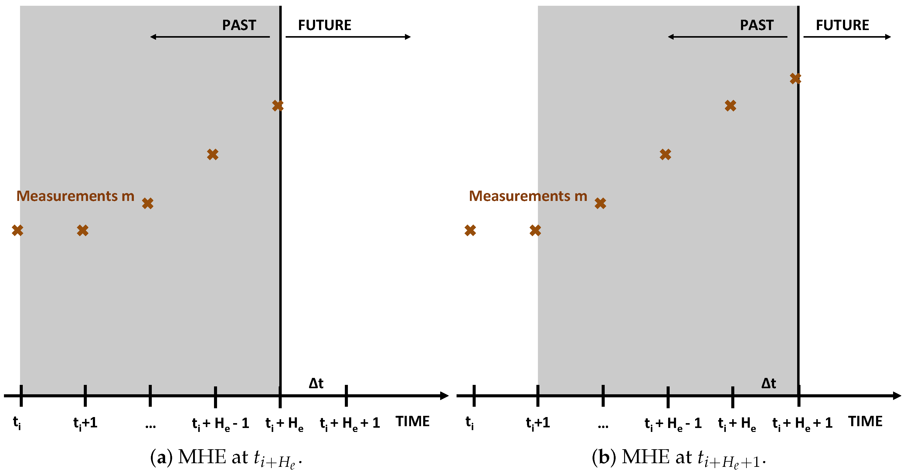
2.2. Moving Horizon Estimation (MHE)

Moving horizon estimation (MHE) estimates states and parameters at a point in time t i + H e from the measurements at this time point and the measurements at the previous H e time points. Hence, an estimation horizon of H e + 1 measurements is used for the state and parameter estimation. Once a new sample is taken at t H e + 1 , the estimation horizon moves one time step, meaning that the measurements at t H e + 1 are used for the state and parameter estimation while the measurements related to the first point of the previous horizon (i.e., t i ) is discarded [12,13,14]. This is also illustrated in Figure 1.
Concretely, a dynamic combined state and parameter estimation problem (in essence, a dynamic optimization problem) is solved over a time interval t i , t i + H e . In this article, the MHE formulation of [7] is used. This formulation is presented below for completeness. For more details on this formulation, the interested reader is referred to [7].
min x H e c , w i , , w i + H e 1 j = i i + H e m j y ( t j ) V 2 + j = i i + H e 1 w j W 2 + x i c x ¯ i c P ¯ i
subject to:
x ˙ ( t ) = S e · K · u ^ ( x , p ) · q bio · x ( t ) + X in · r x ( t ) · D + ω x ( t )
p ˙ ( t ) = ω p ( t )
x ( t i ) = x i
p ( t i ) = p i
0 = z ( t ) I irr · K · u ^ ( x , p )
y ( t ) = x ( t )
x ( t ) 0 , z ( t ) 0
with x ( t ) = c ext ( t ) c bio ( t ) being the state vector comprising both extracellular metabolites and biomass at t, u ^ the estimated free fluxes, p the flux parameters, q bio = 0 0 1 a row vector selecting the partition of the extracellular stoichiometric S e = S ext s bio corresponding with biomass, X in R 4 × 2 the matrix of concentrations at the bioreactor inlet for the different metabolites, and r R 2 × 1 the vector of control variables manipulating the feed composition sent to the reactor and D the dilution rate. In addition, the process noise on the states and parameters is denoted by ω x ( t ) and ω p ( t ) , respectively. Algebraic states z ( t ) have been added for the description of the irreversible fluxes as denoted in Equation (9).
Note that x H e c , i.e., the combined state and parameter vector at t i + H e and the process noise estimates w i , , w i + H e 1 are the optimization variables for the MHE problem described in Equations (4)–(11). Note that the arrival cost parameters x ¯ i c and P ¯ i are updated via an unscented Kalman filter [16].

2.3. Unscented Kalman Filter (UKF)

The unscented Kalman filter (UKF) is an extension of the unscented transformation to the Kalman filter. The unscented transform is a way to calculate the mean and variance of the nonlinear transformation of a random variable that follows a symmetric unimodal distribution. In this article, the states and parameters are the nonlinear transformation of the random variable (i.e., the initial conditions of the states and parameters). In UKF, the sigma points, a fixed number of deterministically chosen sampling points from the distribution of the random variable and are then propagated through the nonlinear function. The mean and covariance of this propagation are subsequently approximated. For the implementation of the UKF in this work, the sigma points are chosen based on recommendations from [11]. Different strategies can be used to select these sigma points and recently a comparative study has been presented in [17].

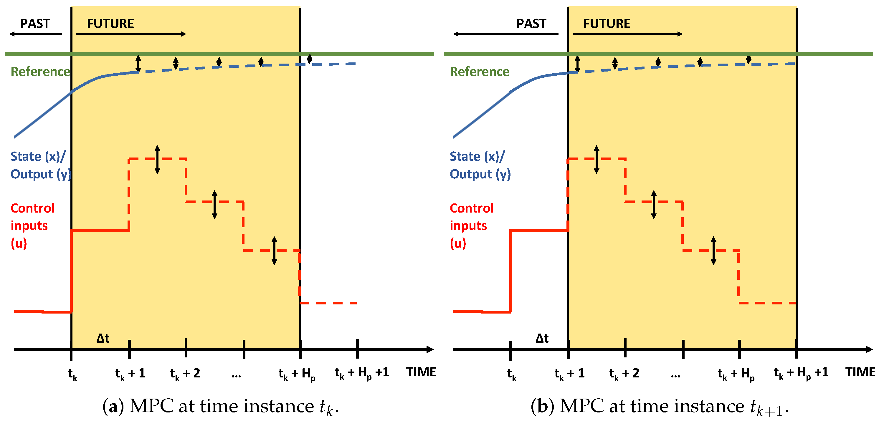
2.4. Model Predictive Control (MPC)

Model predictive control (MPC) solves an open-loop dynamic optimization problem over a time interval t k , t k + H p , with  H p as the prediction horizon to optimize the future of a process. The novel obtained measurements and state and parameter estimates at t k are used as initial conditions for the open-loop dynamic optimization problem that is solved at every iteration. This principle is illustrated in Figure 2: based on the state estimate or measurement at t k a dynamic optimization problem is solved over the time interval t k , t k + H p (a). The solution is applied to the process until a new measurement at t k + 1 is obtained and then a new dynamic optimization problem is solved over t k + 1 , t k + H p + 1 (b).
MPC has become a widespread control strategy and numerous successful applications to industrial problems have been reported, e.g., [18,19]. MPC typically refers to linear MPC in which a quadratic objective function is minimized using a linear process model and subject to linear constraints. In the last decades, nonlinear MPC (NMPC) approaches using nonlinear process models, constraints, and objective functions have become more popular.
In this article the following (N)MPC formulation for t t k , t k + H p is used, based on [20]:
min x ( · ) , u ( · ) t k t k + H p L ( x ( τ ) , u ( τ ) , ) d τ + M ( t k + H p )
subject to:
x ˙ ( t ) = S e · K · u ( x , p ) · q bio · x ( t ) + X in · r x ( t ) · D
p ˙ ( t ) = 0
x ( t k ) = x ^ k
p ( t k ) = p ^ k
0 = z ( t ) I irr · K · u ( x , p )
y ( t ) = x ( t )
x ( t ) 0 , z ( t ) 0
0 c ( x , r , p , t ) .
with x ^ ( t k ) being the measured or estimated state values at t i , c ( x , r , p , τ ) , constraint functions on the systemare not comprised by the previous constraints, τ is the time used in solving the dynamic optimization problems in the NMPC routine, and x and r the states and controls computed by solving the dynamic optimization problem on the interval t k , t k + H p . Note that for the other symbols the same notation is used as in the MHE problem (Equations (4)–(11)). As MPC requires that the entire state vector is known, the states and parameters estimates at t k are denoted by x ^ k and p ^ k .

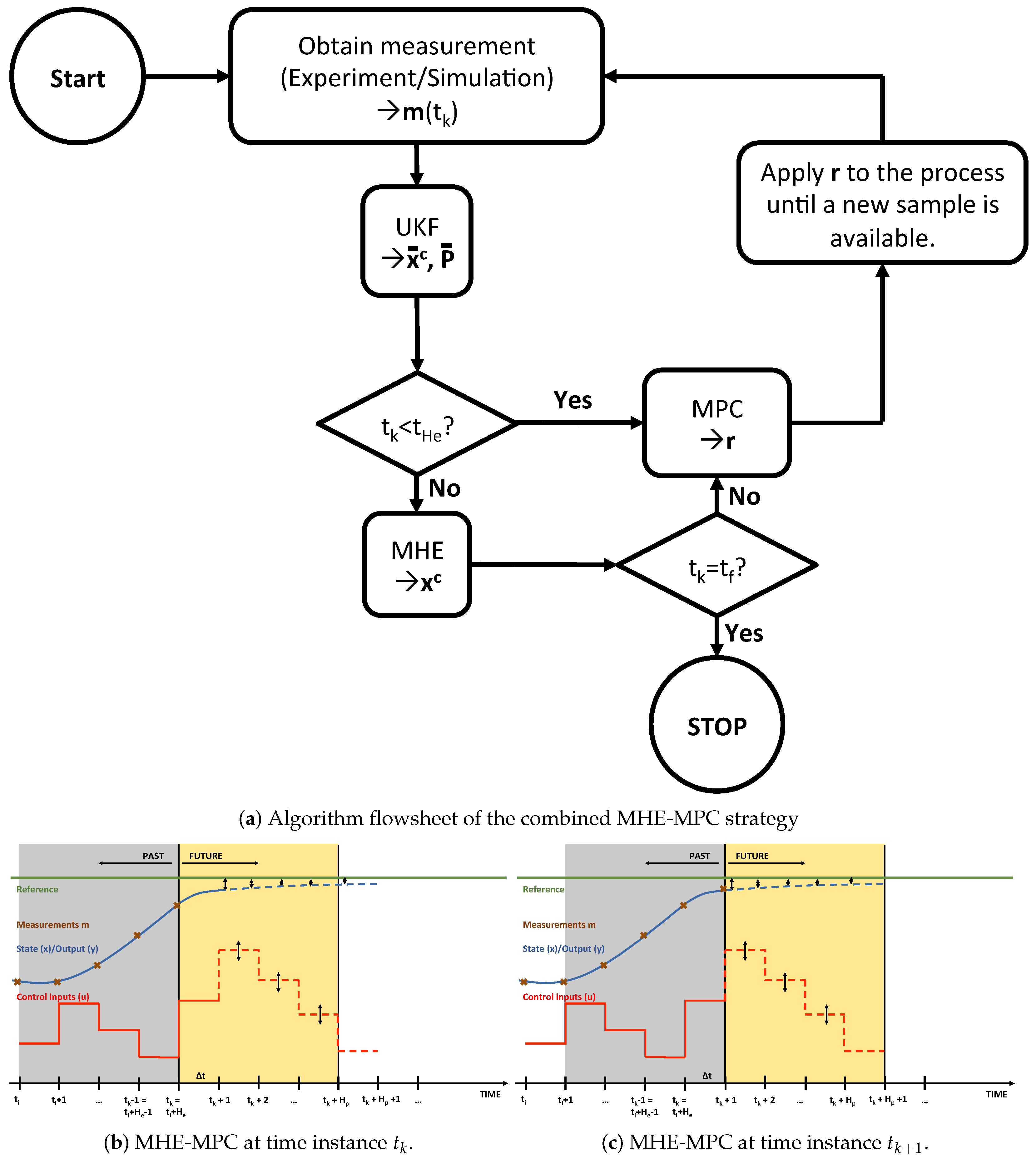
2.5. Combined MHE/MPC Strategy

In this article, a strategy combining MHE and MPC is used for the model-based predictive control of bioprocesses exploiting metabolic network information. The moving-horizon strategy used in this work is thus different from regular implementations because of the black-box nature of the flux models which are used. The proposed strategy is outlined in Figure 3.
The algorithm starts with taking a sample and use an unscented Kalman filter (UKF) to estimate the combined state and parameter vector and the combined state and parameter variance-covariance matrix. Subsequently, it is checked whether a sufficient number of measurements is available to perform MHE, i.e.,  H e + 1 measurements need to be available or equivalently: t k t H e . If  t k < t H e , the state and parameter estimates from UKF are used for the MPC step. Otherwise, the state and parameter estimates from the MHE procedure are used for the MPC step. The control action computed during the MPC step is then applied to the process until the next sample is obtained. Once the end time t f is reached, the algorithm is stopped.
This combined MHE-MPC strategy has been implemented in the Pomodoro toolkit [21], which is available at https://cit.kuleuven.be/biotec/software/pomodoro (accessed on 11 October 2021). Pomodoro is a toolkit that can be used for solving dynamic (multi-objective) optimization problems and for model-based control and estimation. Pomodoro uses CasADi [22] as a symbolic framework for the problem formulation and derivative computation. Orthogonal collocation is used as default to discretize the dynamic optimization problems. A piecewise constant discretization is used for the controls and cubic Lagrange polynomials with collocation points at the Radau roots are used for the states [23]. The resulting NLPs are solved with IPOPT [24].

3. Results and Discussion

The proposed combined MHE-MPC strategy for metabolic network model-based predictive bioprocess control has been implemented on a CSTR bioreactor using a low-complexity metabolic network. The general setup for the implementation of this case study is shown in Figure 4. Two different models are used: (i) the simulation model, which gives the process dynamics, and to which output noise is added to get the process measurements, and (ii) the estimation/control model, which is an approximation since the process model is not known. It is important to note that only the flux kinetics are assumed to be unknown in the estimation/control model. The metabolic reaction network in the estimation/control model is for this case study the same as the one used in the simulation model. Additionally, the general model structure, i.e., the transport terms, etc., are the same for both the simulation and the estimation/control model.

3.1. Case Study Description

The bioprocess in this case study is a continuous bioreactor with two substrates and two products. The composition of the medium that is fed to the bioreactor is controlled, but the flow rate of this feed is always kept constant, as well as the flow rate of the spent medium that is removed from the bioreactor. Since both these flow rates are equal, the volume of the bioreactor is kept constant. Mathematically, the dynamic model consists of (i) the reaction term as defined in Equations (21) and (22), and (ii) transport terms because of the supply of substrate to the reactor and removal of medium from the reactor. The resulting model is the following:
d c ext ( t ) d t = S ext · K · u ( t ) · c bio ( t ) + ( C in · w c ext ) · D
d c bio ( t ) d t = s bio T · K · u ( t ) · c bio ( t ) c bio · D
with F as the flow rate (L/h) in and out of the bioreactor and V the volume (L) of the bioreactor, making D = F V the dilution rate (1/h). In this article, the dilution rate is fixed to 0.1 h 1 . The ( 3 × 3 ) substrate composition matrix C in is made up of three columns that express the composition of each of the three feed mixtures, and the ( 3 × 1 ) control vector w contains the weights of these feeds in the final mixture which is sent to the bioreactor. To make sure the total flow rate to the bioreactor is equal to the outgoing flow rate, these controls should always sum to one:
i = 1 3 w i = 1
This way, there are only two independent controls in the system. The numerical values for the model parameters are given in Table 1.
The metabolic reaction network, simulation model, and the estimation/control model are briefly discussed below.

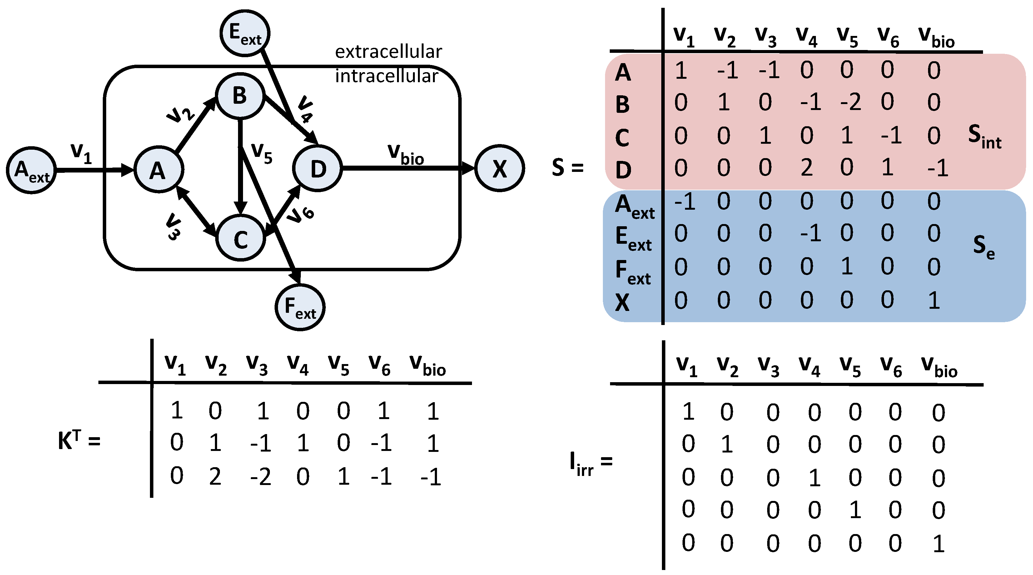
3.1.1. Metabolic Reaction Network

The metabolic reaction network that is used in the case study is shown in Figure 5 on the left, along with the corresponding S int , S e , I irr , and the selected null basis K (note that K is depicted in Figure 5) matrices. It consists of threee extracellular metabolites (A ext , E ext , F ext ) and biomass (X), four intracellular metabolites (A, B, C, D), and seven fluxes ( v 1 , v 2 , v 3 , v 4 , v 5 , v 6 and v bio ). Thus, the number of free fluxes is three.

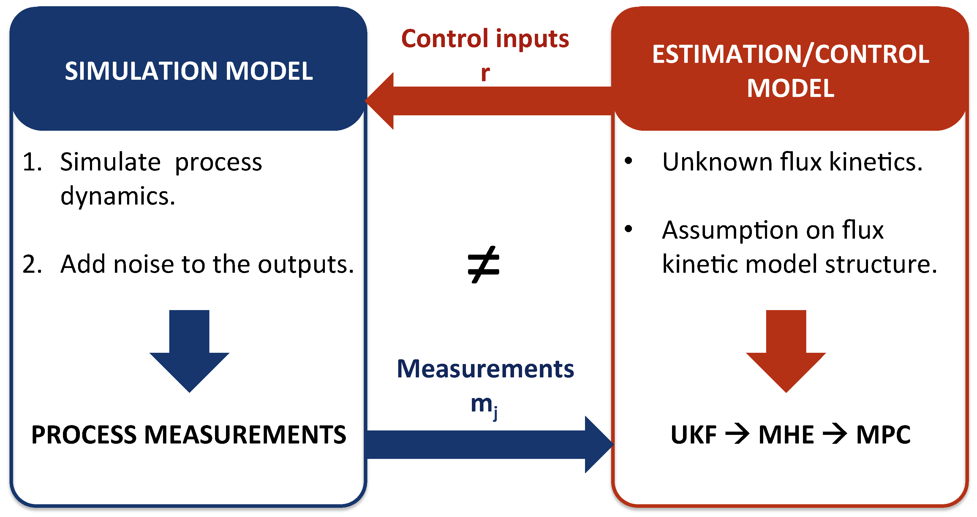
3.1.2. Simulation Flux Model

For the simulation of the measurements, these were chosen as flux 1, 4 and 5. Measurements were simulated by choosing reference profiles for these three fluxes, and simulating the states using the dynamic system.
u 1 , ref = c Aext 1.5 + c Aext
u 4 , ref = 0.2 · c Eext 3 + c Eext
u 5 , ref = 1 1 + c Fext
This simulation flux model is used to generate measurements over a time range of 140 h, measuring A ext , E ext , F ext . Additive, independent, Gaussian measurement noise was added to the output of the simulation model with 0.01 as standard deviation. The initial conditions were set to x 0 = 0.5760 , 3.5527 , 2.4976 , 0.8736 . The process noise was also considered to be of the same type but with a standard deviation of 0.001. The standard deviations to be used in the arrival cost parameters P ¯ 0 is taken equal to the measurement variance for the states and set to 1.0 for the parameters. Different sampling frequencies are studied and the same holds for the prediction and estimation horizons H p and H e , which are chosen to be equal in this article. This is not necessarily the case in practice.

3.1.3. Estimation/Control Flux Model

Three different kinetic flux model structures are studied as estimation/control flux model, a constant, a linear, and a non-linear model.
The constant model considers the fluxes to be constant:
u ( t ) = p u
with p u R d × 1 , thus three parameters to be identified.
In the linear model, the fluxes are just a linear function of the extracellular concentrations:
u ( t ) = C · c ext ( t )
with C as the ( d × m ext ) matrix of parameters that define the linear relationship between fluxes and metabolite concentrations. This results in nine parameters to be identified.
The non-linear kinetics model that is used in this work is the general biological reaction kinetics model of [25]. This model can describe both positive and negative effects of components on reaction rates, and uses only one parameter per component to describe both effects, and one maximum rate parameter per flux, i.e., m ext + 1 × d parameters:
u i ( t ) = u max , i · j = 1 m ext α i j ( c ext , j ( t ) )
with
α i j ( c ext , j ( t ) ) = c ext , j c ext , j + D i j 2 if D i j 0 1 1 + c ext , j · D i j 2 if D i j < 0
In these equations, u max is the ( d × 1 ) vector of maximum rate parameters, and D is the ( d × m ext ) matrix of modulation parameters. If these parameters are positive, they describe a positive activation/saturation effect of the concentrations on the fluxes, if they are negative, an inhibition effect is represented. Hence, 12 parameters need to be identified i.e., 4 parameters per free flux.

3.2. Numerical Results

Initially, the CSTR bioreactor is studied over a period of 140 h with a sampling rate of 1 h, resulting in 140 simulation intervals. During the first 10 h, a constant ratio of 50% A ext and E ext is fed to the CSTR reactor. A horizon length of 4 h has been selected for both the estimation horizon as the prediction horizon (i.e., H = H e = H p = 4 h, corresponding to 20 intervals). This means that after 4 h, the first MPC control action is applied to the process. Moreover, the set point x SP for the MPC is defined as follows:
x SP = 0.5448 , 1.3355 , 3.3852 , 1.4845 if 40 h t k 80 h 0.5760 , 3.5527 , 2.4976 , 0.8736 else

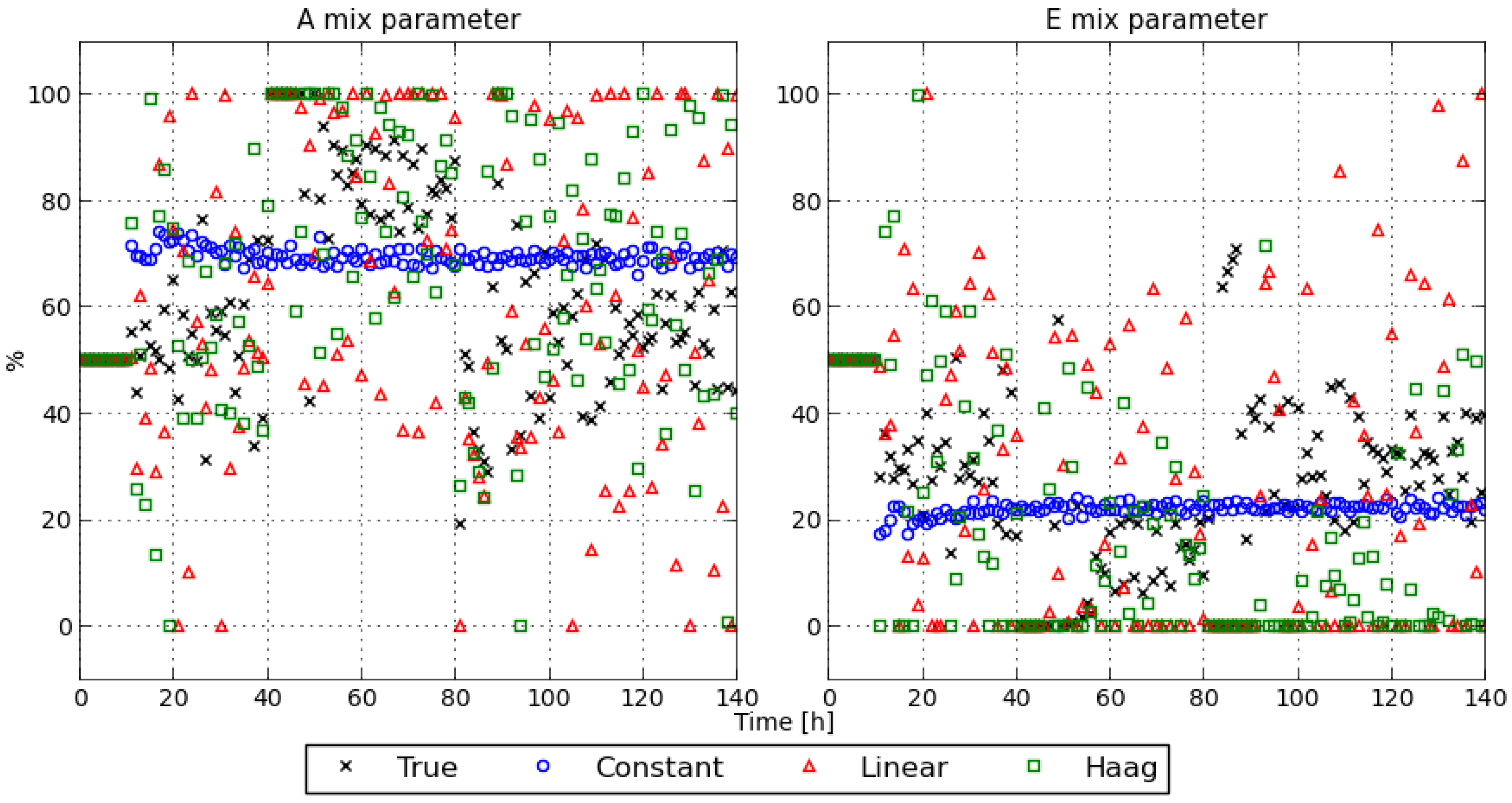
3.2.1. State Estimates

In Figure 6 the simulated state profiles are depicted together with the estimates obtained when using the estimation/control model. The full lines indicate the simulations while the markers indicate the estimates. For all different models the proposed strategy results in accurate state estimates. This complies with the results presented in [7]. For an extensive discussion focusing only on state estimation the interested reader is referred to [7]. Recall that the arrival cost matrices are computed with an unscented Kalman filter in this article, contrary to the arrival cost computation in [7]. In [7] the arrival cost is approximated by a quadratic cost and linearizing the nonlinear functions to obtain a linear least squares problem that can be solved analytically and results in an analytical expression for the arrival cost [14].
A notable difference can be observed when comparing the state profiles for the different flux models. The cause for this difference can be twofold: (i) the linear and Haag models are more similar to the true flux model than the constant flux model hence resulting in more similar flux profiles, and (ii) the control profiles for the true, linear, and nonlinear flux models are more similar, compared with the constant flux model. This is investigated in more depth below.

3.2.2. MPC Tracking Performance

In Figure 7 the extracellular metabolite concentration profiles (i.e., the state profiles) are depicted for the different methods, together with the set point that is used for the different concentrations during the MPC procedure. For the extracellular metabolites that are consumed, i.e., A ext and E ext , the set points are better tracked by the true flux model and the constant flux model than by the linear and Haag models. The extracellular metabolites that are excreted (or produced) by the cells are better approximated with the true, linear, and Haag flux models. These observations are made from Figure 7.
In order to quantify the difference in tracking performance between the MPC control strategies obtained with the different flux models, the unscaled absolute values of the absolute tracking errors for each state are depicted in Table 2. From this table it becomes clear that the constant model has the lowest tracking error for the first state A ext . For E ext the tracking error is the lowest for the true flux model, while the constant and linear models perform slightly worse. The Haag model performs the worst for E ext . F ext is comparably well tracked by the true model, linear model, and Haag model. The constant flux model has a poor tracking for F ext . The biomass concentration is well tracked by the true model, linear model, and Haag model, while the constant model is again performing poorly. These observations confirm the observations made from Figure 7.
For completeness, the control profiles are depicted in Figure 8. The control profiles computed with the constant flux model are flatter than the control profiles computed with the other flux models. The difference between these control profiles confirms the tracking performance discussed above.

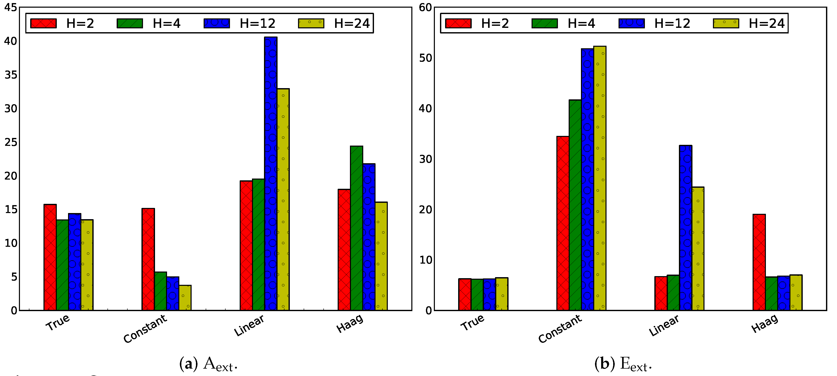
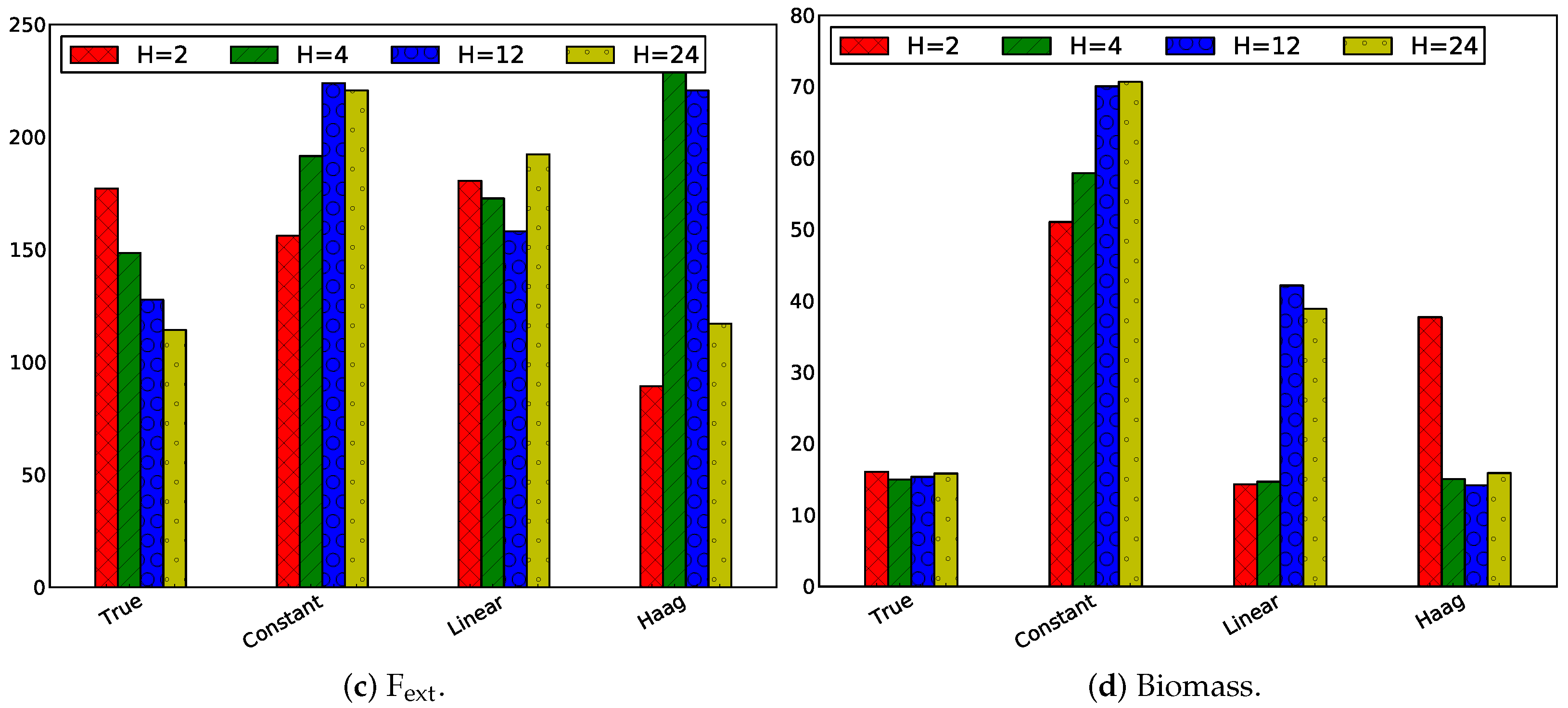
3.2.3. Influence of Horizon Length

Same Horizon and Estimation Horizon

Firstly, the influence of the horizon length on the tracking performance is studied by selecting the same horizon for estimation and prediction (control): H = H e = H p . Four different horizons have been simulated, assuming that a sample is taken every hour: H = 2 h , H = 4 h , H = 12 h , H = 24 h . The absolute values of the absolute tracking error for all states are depicted in Figure 9.
Globally, it can be observed that the MPC control performance obtained with the true flux model and the linear flux model are more similar for a small horizon length, i.e., H = 1 h. However, no clear global trends can be observed for the increase of the horizon length. As both the estimation and prediction horizon have been modified, it is difficult to interpret these graphs. Therefore the effect of only changing the prediction horizon or solely changing the estimation horizon is addressed in the next paragraphs.

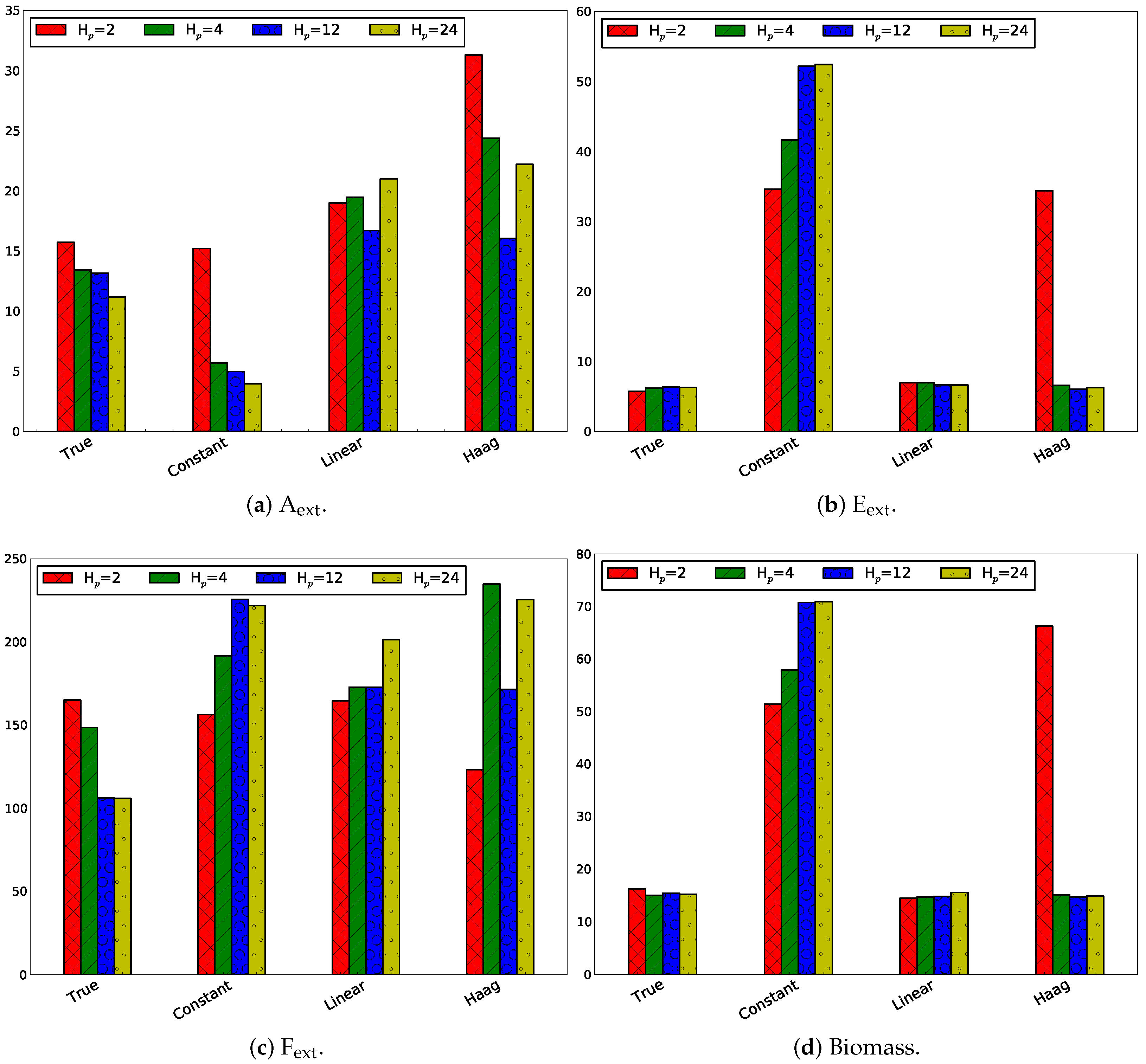
Influence of Only Changing the Prediction Horizon

In this paragraph the estimation horizon is set to H e = 4 h and the prediction horizon has been varied as in the previous paragraph. Four different horizons have been simulated, assuming that a sample is taken every hour: H p = 2 h , H p = 4 h (4 h), H p = 12 h , H p = 24 h . In Figure 10, the absolute values of the absolute tracking error are displayed.
Increasing the prediction horizon results in a slight reduction of the tracking error of all states using the true flux model. For the other flux models, such clear observations cannot be made.

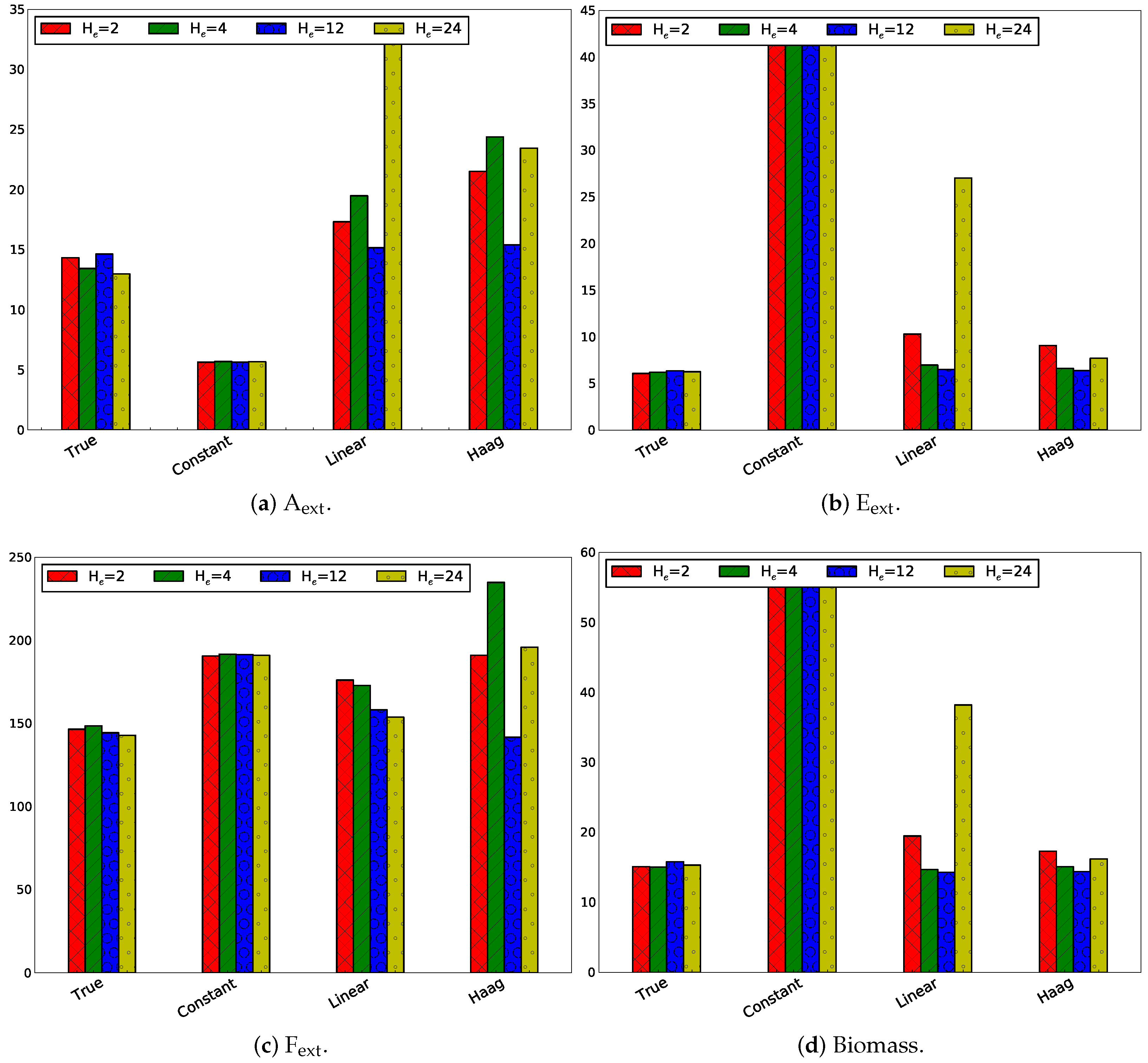
Influence of Only Changing the Estimation Horizon

Contrary to the previous paragraph, the estimation horizon is varied and the prediction horizon is kept constant at 4 h. Following estimation horizons have been studied for a sampling rate of 1 h: H e = 2 h , H e = 4 h (4 h), H e = 12 h , H e = 24 h . In Figure 11, the absolute values of the absolute tracking error are displayed.
The estimation horizon has a small effect on the MPC tracking performance, except for the linear flux model, in which the estimation horizon of 24 h clearly results in a higher on the MPC tracking error for all extracellular metabolites except F ext .

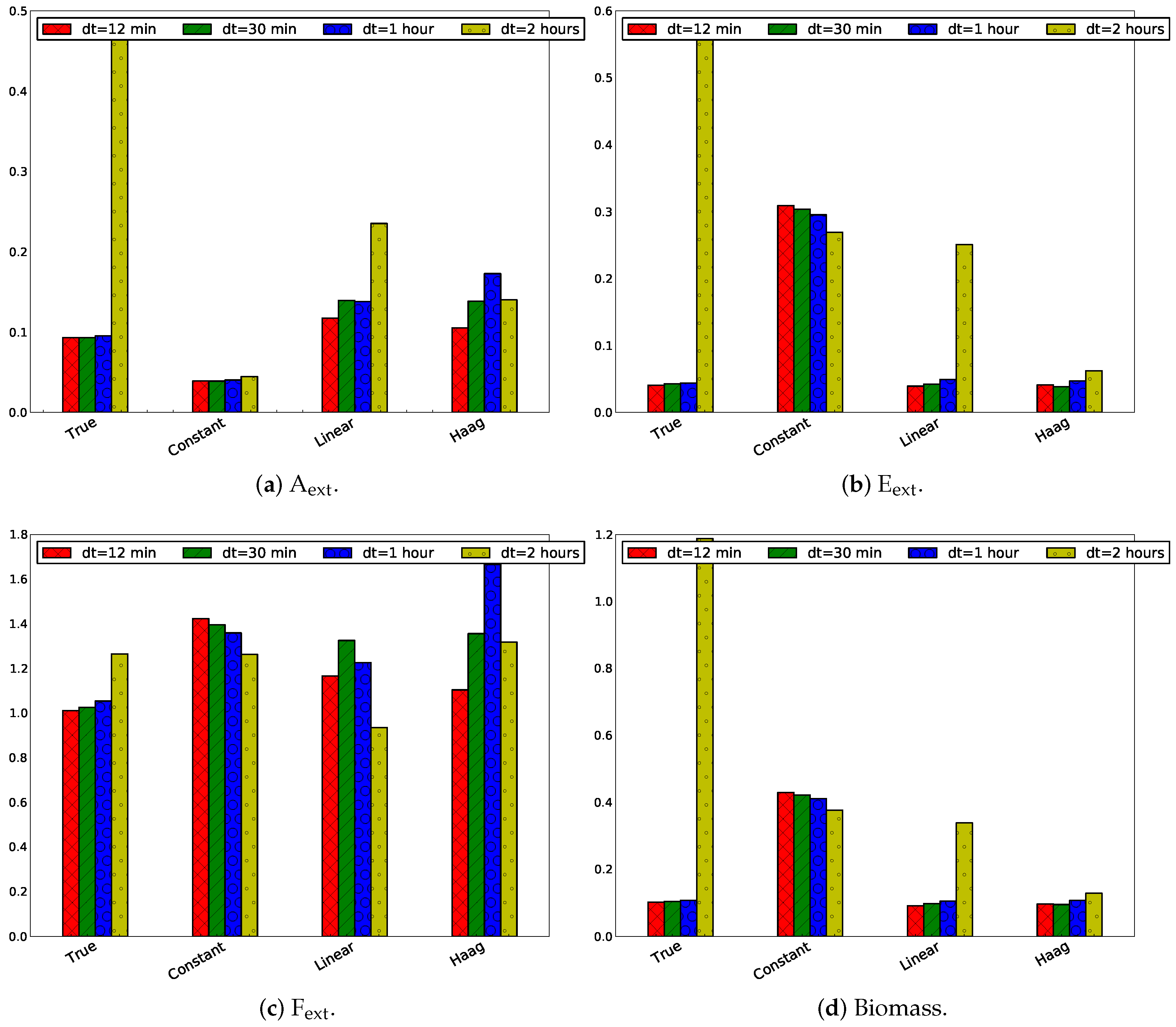
3.2.4. Influence of Sampling Frequency

The influence of the sampling frequency on the tracking performance has been studied for an estimation and horizon length of 4 h ( H = H e = H p = 4 h). Four sampling frequency scenarios have been studied: 12 min, 30 min, 1 h, and 2 h. The MPC tracking error divided by the number of sampling points has been depicted in Figure 12.
It is expected that a higher sampling frequency will result in better tracking. This corresponds with lower sampling times d t . In Figure 12 this is only observed for the true model. For the linear model this is the case for all states, except F ext . In the Haag model, this is not observed for E ext . A lower sampling frequency only results in a better tracking for the constant flux model for A ext .

4. Conclusions

One of the current limitations in online bioprocess control is the use of macroscopic models (that only account for substrate, biomass, and product mass balances), as the available process knowledge on the relevant underlying intracellular mechanisms is not fully exploited and as such opportunities are missed towards an optimal bioprocess operation. In this article, a procedure for metabolic network-based model predictive control has been presented, by combining online flux estimation and bioprocess control using metabolic network models. This procedure firstly uses moving horizon estimation (MHE) to estimate the states and fluxes from the available measurements and subsequently solves a model predictive control (MPC) problem to determine the optimal control strategy for the studied bioprocess. To illustrate the performance of this procedure, a case study combining a CSTR bioreactor model with a metabolic network model has been implemented. Three different model structures (a constant, a linear, and a nonlinear model) have been compared, clearly indicating that the linear flux model outperforms the nonlinear Haag flux model and the constant flux model. The true model is, as expected, outperforming the other models. In addition, the influence of the horizon lengths and sampling frequency on the MPC tracking performance has been studied. While an increase of the prediction horizon length was expected to reduce the tracking error, such observation could only be made for the true model. An increase in sampling frequency (or reduction in sampling time) was expected to reduce the tracking error, but this observation could only be made for the true model and for the linear model.
In future work, the presented procedure will be applied to the online control of bioprocesses involving large-scale metabolic networks. In addition, uncertainty will be accounted for during the MPC routine. Furthermore, the presented metabolic network-based model predictive control procedure can also be combined with high-throughput biological datasets [26,27] and advanced metabolomics techniques as e.g., low-frequency NMR, to improve the metabolic model predictions and process monitoring capabilities [8,27]. One of the current limitations of metabolic network models and methods as metabolic flux analysis is the inherent pseudo-steady state assumption. This assumption is not always valid, certainly not at timescales of multiple scales due to shifting from exponential growth phase to stationary phase. The authors of [28] proposed a hybrid modeling approach, combining machine learning with metabolic network modeling which provided accurate predictions for amino acid consumption rates in Chinese Hamster Ovary Cells. Such hybrid models could also be used in the proposed metabolic network-based MPC procedure.

Author Contributions

Conceptualization, P.N., D.V., S.B., F.L. and J.V.I.; methodology, P.N. and D.V.; software, P.N., D.V. and S.B.; validation, P.N. and S.B.; formal analysis, P.N.; investigation, P.N. and D.V.; resources, F.L. and J.V.I.; data curation, P.N.; writing—original draft preparation, P.N.; writing—review and editing, P.N., S.B., F.L. and J.V.I.; visualization, P.N. and S.B.; supervision, F.L. and J.V.I.; project administration, F.L. and J.V.I.; funding acquisition, F.L. and J.V.I. All authors have read and agreed to the published version of the manuscript.

Funding

This work was supported by KU Leuven Center-of-Excellence Optimization in Engineering (OPTEC), projects G086318N and G0B4121N of the Fund for Scientific Research Flanders (FWO), the European Commission within the framework of the Erasmus+ FOOD4S Programme (Erasmus Mundus Joint Master Degree in Food Systems Engineering, Technology and Business 619864-EPP-1-2020-1-BE-EPPKA1-JMD-MOB) and by the European Union’s Horizon 2020 Research and Innovation programme under the Marie Skłodowska-Curie Grant Agreement N956126 (E-MUSE Complex microbial Ecosystems MUltiScale modElling). The APC was funded by FWO G0B4121N.

Institutional Review Board Statement

Not applicable.

Informed Consent Statement

Not applicable.

Conflicts of Interest

The authors declare no conflict of interest.

Abbreviations

The following abbreviations are used in this manuscript:
CSTRContinuous stirred tank reactor
DMFADynamic metabolic flux analysis
MFAMetabolic flux analysis
MHEMoving horizon estimation
MPCModel predictive control

References

  1. Szallasi, Z.; Stelling, J.; Periwal, V. System Modeling in Cell Biology; MIT Press: Cambridge, MA, USA, 2006. [Google Scholar]
  2. Llaneras, F.; Picó, J. Stoichiometric modelling of cell metabolism. J. Biosci. Bioeng. 2008, 105, 1–11. [Google Scholar] [CrossRef] [PubMed]
  3. Chang, L.; Liu, X.; Henson, M.A. Nonlinear model predictive control of fed-batch fermentations using dynamic flux balance models. J. Process Control 2016, 42, 137–149. [Google Scholar] [CrossRef]
  4. Leighty, R.W.; Antoniewicz, M.R. Dynamic metabolic flux analysis (DMFA): A framework for determining fluxes at metabolic non-steady state. Metab. Eng. 2011, 13, 745–755. [Google Scholar] [CrossRef] [PubMed]
  5. Martínez, V.S.; Buchsteiner, M.; Gray, P.; Nielsen, L.K.; Quek, L.E. Dynamic metabolic flux analysis using B-splines to study the effects of temperature shift on CHO cell metabolism. Metab. Eng. Commun. 2015, 2, 46–57. [Google Scholar] [CrossRef] [PubMed]
  6. De Sousa, S.F.; Bastin, G.; Jolicoeur, M.; Wouwer, A.V. Dynamic metabolic flux analysis using a convex analysis approach: Application to hybridoma cell cultures in perfusion. Biotechnol. Bioeng. 2015, 113, 1102–1112. [Google Scholar] [CrossRef] [PubMed]
  7. Vercammen, D.; Logist, F.; Van Impe, J. Online moving horizon estimation of fluxes in metabolic reaction networks. J. Process Control 2016, 37, 1–20. [Google Scholar] [CrossRef] [Green Version]
  8. Liu, P.; Hua, Y.; Zhang, W.; Xie, T.; Zhuang, Y.; Xia, J.; Noorman, H. A new strategy for dynamic metabolic flux estimation by integrating transient metabolome data into genome-scale metabolic models. Bioprocess Biosyst. Eng. 2021. [Google Scholar] [CrossRef]
  9. Kalman, R. A New Approach to Linear Filtering and Prediction Problems. Trans. ASME-J. Basic Eng. 1960, 82, 35–45. [Google Scholar] [CrossRef] [Green Version]
  10. Becerra, V.; Roberts, P.; Griffiths, G. Applying the extended Kalman filter to systems described by nonlinear differential-algebraic equations. Control Eng. Pract. 2001, 9, 267–281. [Google Scholar] [CrossRef]
  11. Julier, S.; Uhlmann, J. A General Method for Approximating Nonlinear Transformations of Probability Distributions; Technical Report; Robotics Research Group, Department of Engineering Science, University of Oxford: Oxford, UK, 1996. [Google Scholar]
  12. Robertson, D.G.; Lee, J.H.; Rawlings, J.B. A moving horizon-based approach for least-squares estimation. AIChE J. 1996, 42, 2209–2224. [Google Scholar] [CrossRef]
  13. Rao, C.V.; Rawlings, J.B. Constrained process monitoring: Moving-horizon approach. AIChE J. 2002, 48, 97–109. [Google Scholar] [CrossRef]
  14. Kühl, P.; Diehl, M.; Kraus, T.; Schlöder, J.P.; Bock, H.G. A real-time algorithm for moving horizon state and parameter estimation. Comput. Chem. Eng. 2011, 35, 71–83. [Google Scholar] [CrossRef]
  15. Vercammen, D.; Logist, F.; Van Impe, J. Dynamic estimation of specific fluxes in metabolic networks using non-linear dynamic optimization. BMC Syst. Biol. 2014, 8, 1–22. [Google Scholar] [CrossRef] [PubMed]
  16. Qu, C.C.; Hahn, J. Computation of arrival cost for moving horizon estimation via unscented Kalman filtering. J. Process Control 2009, 19, 358–363. [Google Scholar] [CrossRef]
  17. Maußner, J.; Freund, H. Optimization under uncertainty in chemical engineering: Comparative evaluation of unscented transformation methods and cubature rules. Chem. Eng. Sci. 2018, 183, 329–345. [Google Scholar] [CrossRef]
  18. Rawlings, J. Tutorial overview of model predictive control. IEEE Control Syst. Mag. 2000, 20, 38–52. [Google Scholar]
  19. Diehl, M.; Bock, H.; Schlöder, J.; Findeisen, R.; Nagy, Z.; Allgöwer, F. Real-time optimization and nonlinear model predictive control of processes governed by differential-algebraic equations. J. Process Control 2002, 12, 577–585. [Google Scholar] [CrossRef]
  20. Allgöwer, F.; Findeisen, R.; Ebenbauer, C. Nonlinear Model Predictive Control. In UNESCO Encyclopedia of Life Support Systems (EOLSS); EOLSS Publishers Co., Ltd.: Paris, France, 2003; Volume XI. [Google Scholar]
  21. Bhonsale, S.; Telen, D.; Vercammen, D.; Vallerio, M.; Hufkens, J.; Nimmegeers, P.; Logist, F.; Impe, J.V. Pomodoro: A Novel Toolkit for Dynamic (MultiObjective) Optimization, and Model Based Control and Estimation. IFAC-PapersOnLine 2018, 51, 719–724. [Google Scholar] [CrossRef]
  22. Andersson, J.; Akesson, J.; Diehl, M. CasADi—A symbolic package for automatic differentiation and optimal control. In Proceedings of the 6th International Conference on Automatic Differentiation, Fort Collins, CO, USA, 23–27 July 2012. [Google Scholar]
  23. Biegler, L.T. An overview of simultaneous strategies for dynamic optimization. Chem. Eng. Process. Process Intensif. 2007, 46, 1043–1053. [Google Scholar] [CrossRef]
  24. Wächter, A.; Biegler, L.T. On the implementation of an interior-point filter line-search algorithm for large-scale nonlinear programming. Math. Program. 2006, 106, 25–57. [Google Scholar] [CrossRef]
  25. Haag, J.E.; Vande Wouwer, A.; Remy, M. A general model of reaction kinetics in biological systems. Bioprocess Biosyst. Eng. 2005, 27, 303–309. [Google Scholar] [CrossRef]
  26. Duarte, N.C.; Becker, S.A.; Jamshidi, N.; Thiele, I.; Mo, M.L.; Vo, T.D.; Srivas, R.; Palsson, B.O. Global reconstruction of the human metabolic network based on genomic and bibliomic data. Proc. Natl. Acad. Sci. USA 2007, 104, 1777–1782. [Google Scholar] [CrossRef] [PubMed] [Green Version]
  27. Leenders, J.; Grootveld, M.; Percival, B.; Gibson, M.; Casanova, F.; Wilson, P.B. Benchtop Low-Frequency 60 MHz NMR Analysis of Urine: A Comparative Metabolomics Investigation. Metabolites 2020, 10, 155. [Google Scholar] [CrossRef] [Green Version]
  28. Schinn, S.M.; Morrison, C.; Wei, W.; Zhang, L.; Lewis, N.E. A genome-scale metabolic network model and machine learning predict amino acid concentrations in Chinese Hamster Ovary cell cultures. Biotechnol. Bioeng. 2021, 118, 2118–2123. [Google Scholar] [CrossRef] [PubMed]
Figure 1. Illustration of two consecutive MHE iterations.
Applsci 11 09532 g001
Figure 2. Illustration of two consecutive MPC iterations.
Applsci 11 09532 g002
Figure 3. Overview of the combined MHE-MPC strategy: (a) algorithm, (b) combined MHE-MPC at t k , and (c) combined MHE-MPC at t k + 1 .
Applsci 11 09532 g003
Figure 4. General setup with simulation model and estimation/control model.
Applsci 11 09532 g004
Figure 5. Metabolic network and characterizing matrices for the CSTR bioreactor case study.
Applsci 11 09532 g005
Figure 6. Simulated and estimated concentration profiles with the different flux models.
Applsci 11 09532 g006
Figure 7. Concentrations and set points for the different extracellular metabolites, obtained with the different flux models.
Applsci 11 09532 g007
Figure 8. MPC control actions obtained with the different flux models.
Applsci 11 09532 g008
Figure 9. Absolute values of the absolute tracking error in case of H = H e = H p for the four states, i.e., the extracellular metabolite concentrations.
Applsci 11 09532 g009aApplsci 11 09532 g009b
Figure 10. Absolute values of the absolute tracking error in case of H e = 4 h for the four states, i.e., the extracellular metabolite concentrations.
Applsci 11 09532 g010
Figure 11. Absolute values of the absolute tracking error in case of H e = 4 h for the four states, i.e., the extracellular metabolite concentrations.
Applsci 11 09532 g011
Figure 12. Absolute values of the absolute tracking error divided by the number of measurements for the four states for different sampling times with H = H e = H p = 4 h .
Applsci 11 09532 g012
Table 1. Model parameter values.
Model ParameterNumerical Value
F 0.1 L/h
V 1.0 L
C in 6.0 0.0 0.0 0.0 9.0 0.0 0.0 0.0 0.0 mol/L
Table 2. Absolute values of the absolute tracking errors, i.e., difference between state and set point.
TrueConstantLinearHaag
A ext 13.445.6919.4824.38
E ext 148.52191.61172.80234.86
F ext 14.9957.8714.6615.06
Biomass6.1941.646.966.62
Publisher’s Note: MDPI stays neutral with regard to jurisdictional claims in published maps and institutional affiliations.

