An Integrated Software for Computing Mechanical Properties of Crystalline Material by Means of XRD

Abstract

An integrated software for calculating the major mechanical properties of materials was newly programmed. The material mechanical properties are determined from a peak position and the broadness of X-ray diffraction (XRD) line using profile function method, including Gaussian, Parabola, Half-width, and Centroid. The X-ray diffraction line in software is also corrected by the generalized X-ray absorption function. The results show that the precision coefficient (R²) of the d_hkl-sin² ψ linear regression depends on tested materials and the method of the 2θ determination. The Parabola and Gaussian methods show greater fitting accuracy in comparison to the other two methods in determining stress. The mechanical properties calculated using this software agreed well with the values determined from the conventional methods. In addition, this XRD software also allows computing the 95% confidential limits of the results from a single measurement without conducting repetitive measurements. Therefore, the new software allows widening the experimental scopes of an X-ray diffraction device in both laboratories and the industrial sector.

1. Introduction

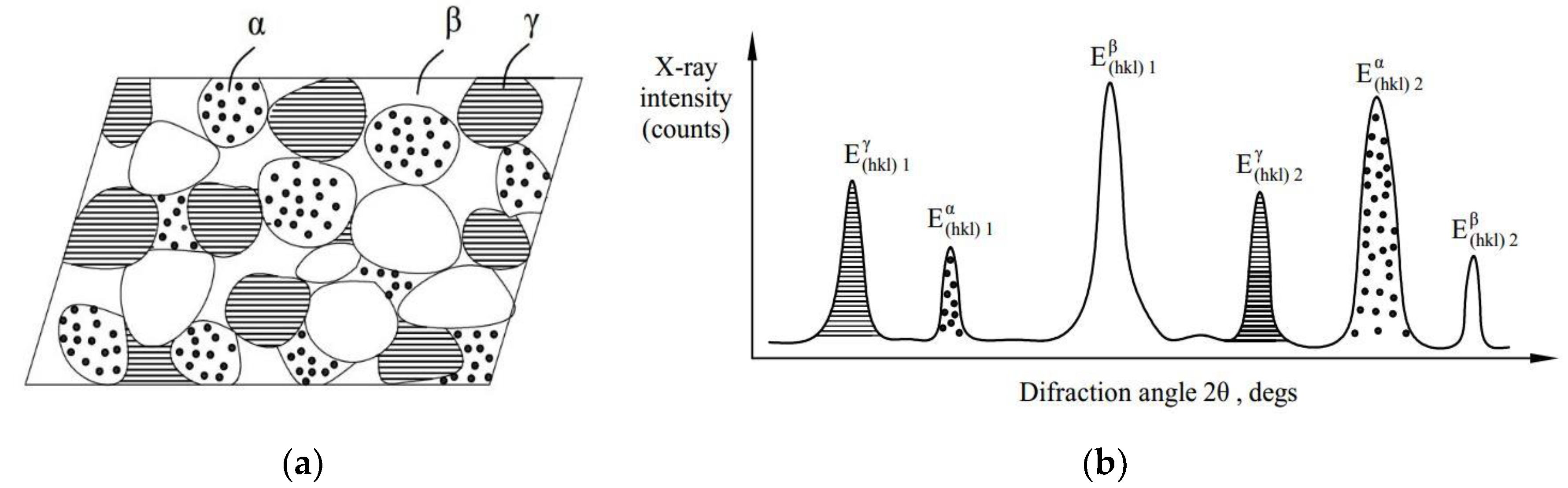
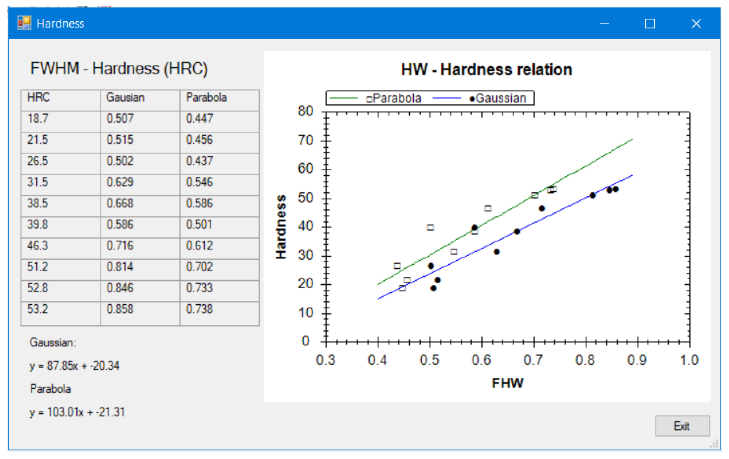
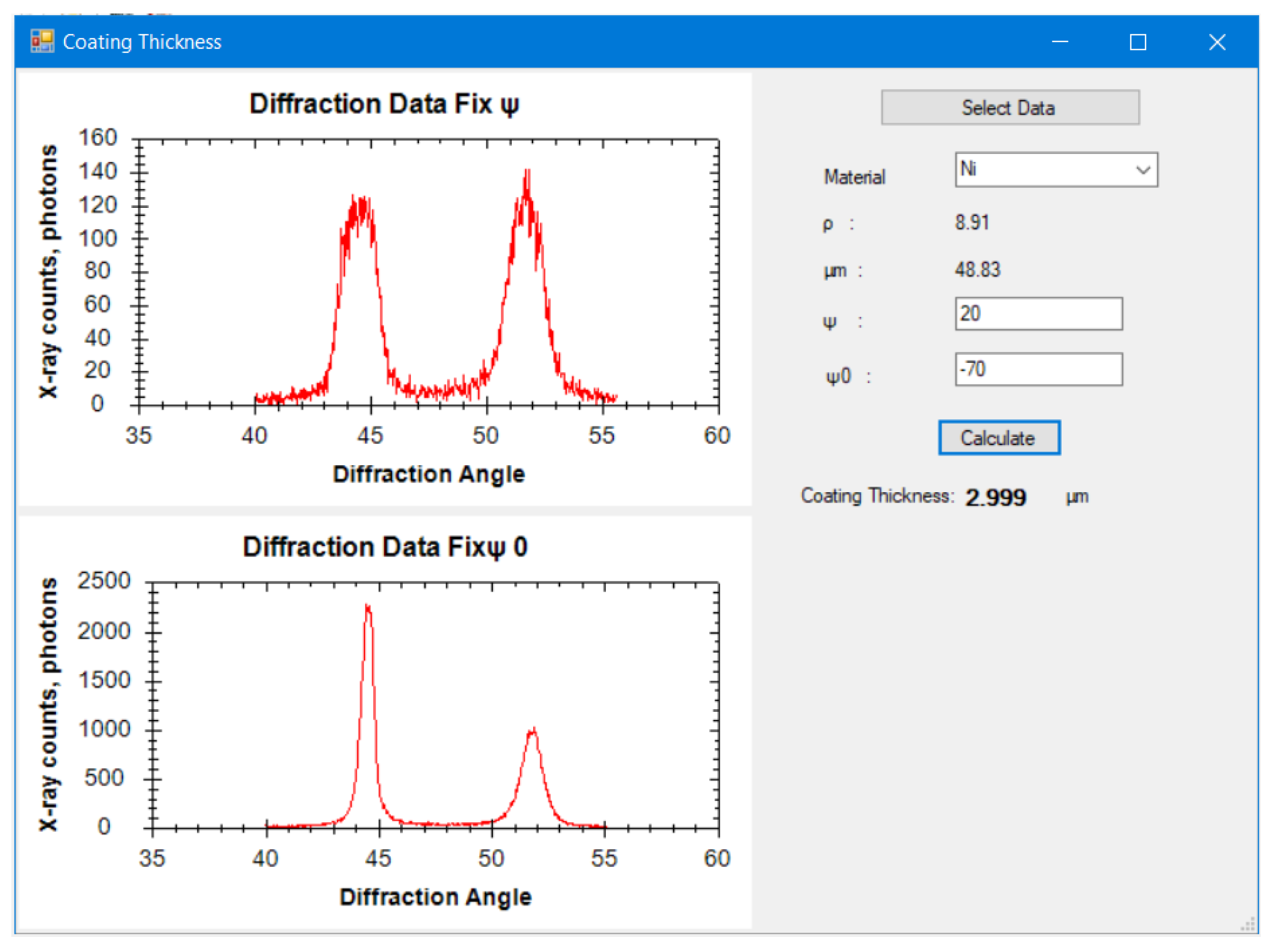
Since they were discovered in 1890, X-rays and the techniques using X-ray diffraction [1,2] have shown great progress and have seen a variety of applications in industry because of their advantages over other nondestructive techniques. They can evaluate many mechanical properties including stress [2,3,4], crystalline grain size [5], phase composition analysis [6,7], hardness [8], the thickness of plating or coating layer [9,10], etc. Moreover, X-ray diffraction has also been used to identify modifications of phase, texture, dislocation density, and mechanical twins of materials [11]. Ultrasonic and magnetic techniques have many applications for many kinds of materials at the macro level to determine material inhomogeneity; however, they cannot determine the properties at the micro- and nano-level. The laser technique can only determine the outer profile of the sample surface such as roughness. The microscopic technique is used to observe crystalline microstructure, and when combined with image processing, it can determine crystal grain size, phase components in multi-phase materials, and layer thickness [12]; however, it has difficulty in determining the state of materials such as stress, hardness, etc. Fortunately, X-rays with short wavelengths can detect the change or characteristics of a crystalline matrix from macro- to micro- and even nano-level, and it can therefore determine the hereabove parameters of crystalline materials. Moreover, a distinguished advantage of the XRD method over the other methods is that it can determine the standard deviations from a single measurement without replication of measurement. This is because the diffraction of photons in the crystal matrix occurs in all directions, and thus functions calculated from X-ray counting, such as peak position, stress, line width, and others, are random functions and contain coherent reproducibility of measured values [13,14].

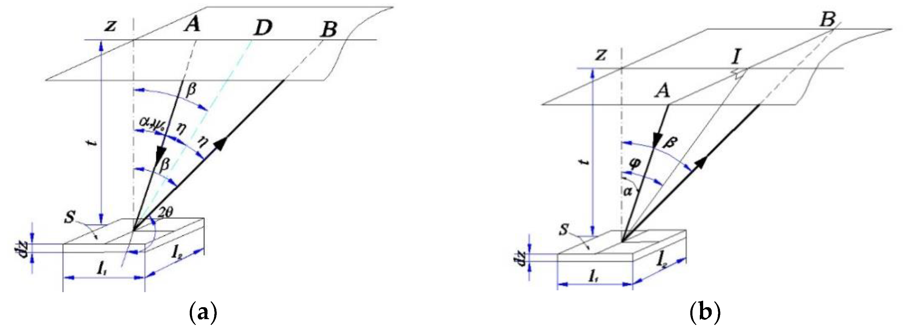
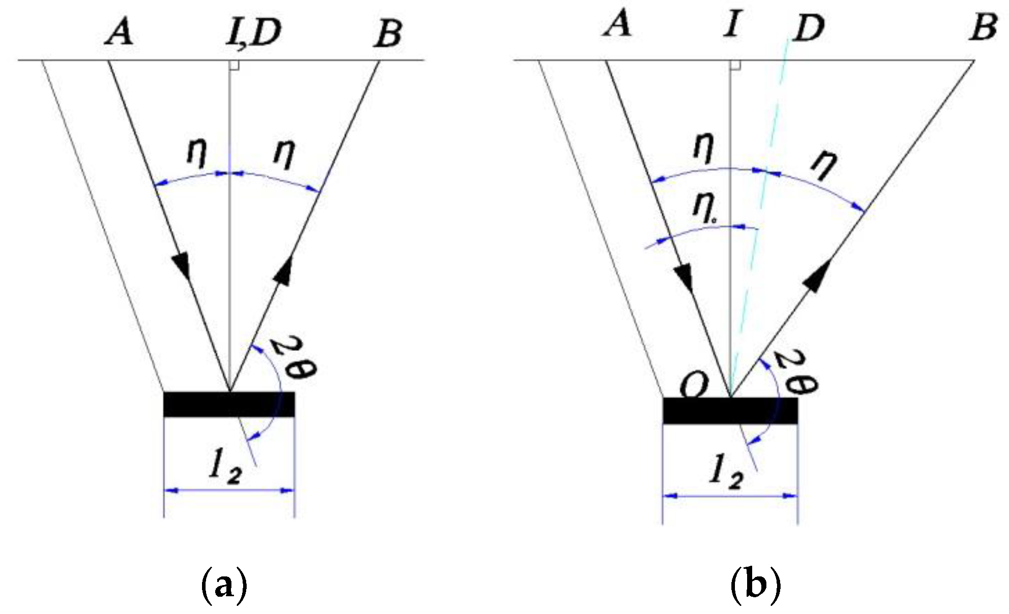
On the other hand, in order to obtain the correct value of X-ray intensity, and thus the accurate peak position and the full width at half of the diffraction line, the diffracted X-ray intensity must be corrected for the Lorentz-polarization and absorption factor [2,15,16]. The absorption factor for only the iso-inclination method (Ω-type goniometer) using the fixed-ψ method was computed and widely used [16]. 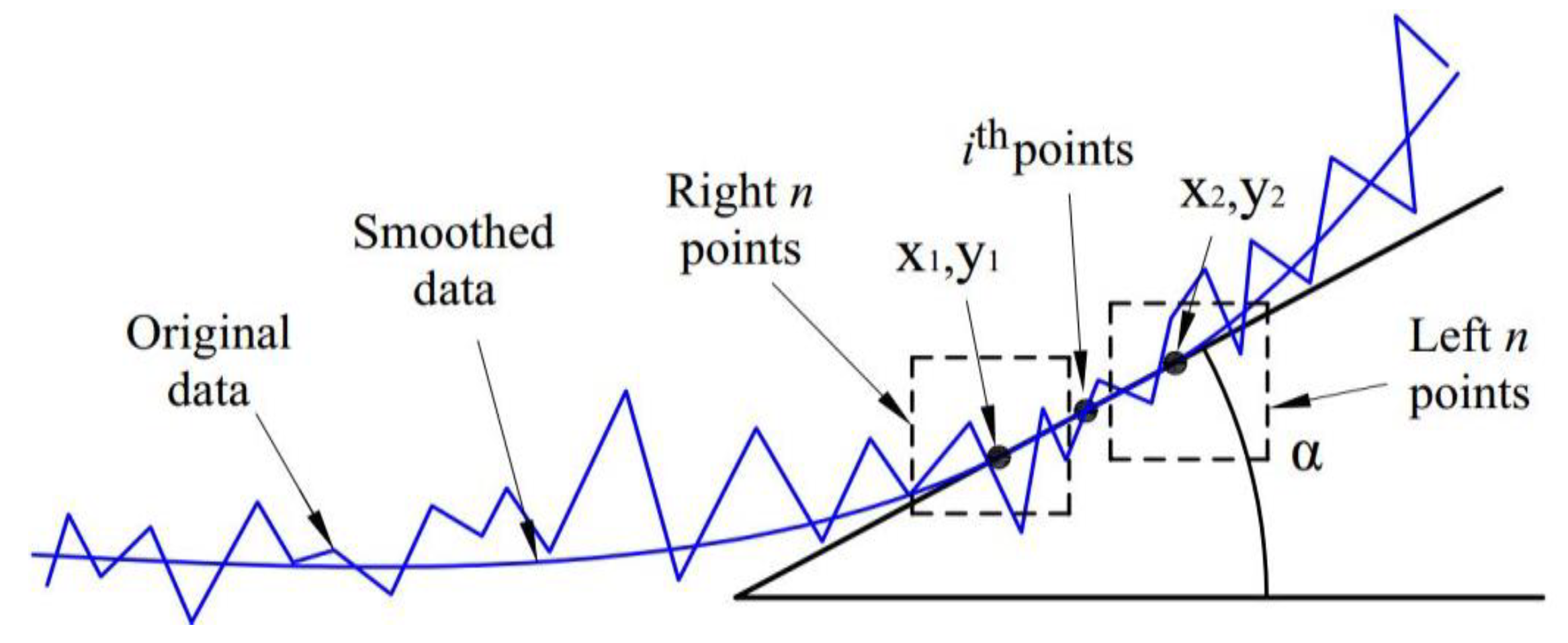However, the position-sensitive proportional counter (PSPC), in which the incident beams are fixed during the scanning process (fixed-ψ₀ method), is used more widely. Moreover, to increase the diffraction angle 2θ up to approximately 170° and the inclination angle ψ up to approximately 165°, the side-inclination method (Ψ-type goniometer) is used. For these measurement methods, the absorption factor is still not fully derived and is not embedded in commercial X-ray systems. Furthermore, there are many methods of approximating the diffraction line to determine the diffraction peak. The choice of mathematical function to interpolate the peak diffraction greatly affected the accuracy of the measurement results. This has been reported in stress measurements using X-ray diffraction (XRD) [17,18]. To enlarge the scope of application of XRD for various measurements in a single device, there should be a computation system that can accurately determine many material properties. 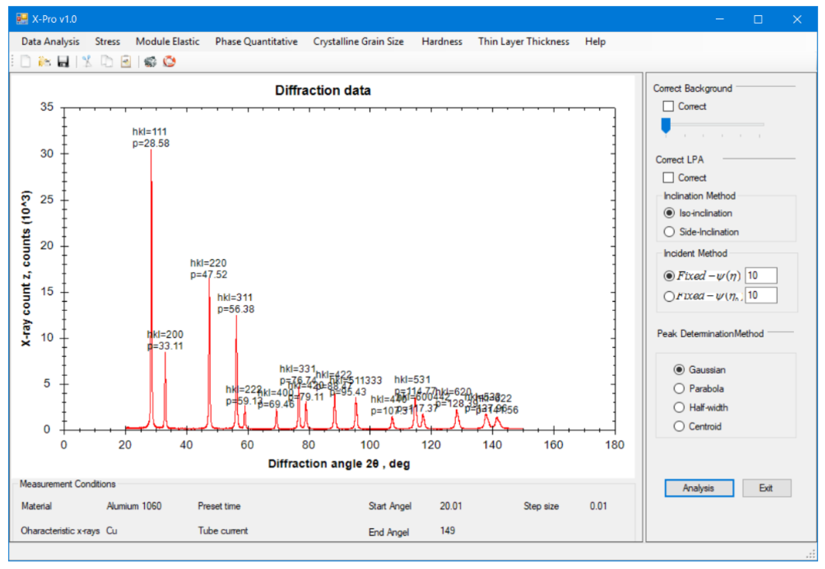In a previous study, automated controlling and calculating software using C++ and commercial MS Excel was used for determining the residual stress of polycrystalline materials [13]. This research represents a new computation program for polycrystalline materials that determines their properties using XRD, with total integration of absorption factors and mathematical function for the correction of diffraction lines. It can evaluate common mechanical properties in industry. The following measurements are carried out:

• Residual stress computation for the aluminum alloy A1060;
• Surface hardness of quenched and tempered carbon steel JIS-type S50C;
• Quantitative analysis for triple-phase carbide T15K6 containing three phases, WC, TiC, and Co;
• Thickness measurement of the nickel-coating layer on substrate carbon steel S45C;
• Determining grain size of the zeolite material ZSM-5.

The demonstration measurements using X-rays and conventional methods were also compared to verify the validity of the computation and thus the applicability to the manufacturing site. All XRD measurements in this study use the X-ray characteristic CuKα with a wavelength λ of 1.5 Å and Ni foil filter. The use of a graphical user interface (GUI) also allows beginner-level programmers to easily reprogram resource codes for their individual computation.

2. Material Analyzing Software

2.1. Selection of Development Language

Structured programming (SP) languages such as Basic, Pascal, and C have a common structure [19]:

Programs = Data structures + Algorithms

The advantage of SP includes ease of following; however, for large projects, the resource code cannot be reused and the algorithm strictly depends on the data structure. In contrast, object-oriented programming languages, including Turbo Pascal, C++, and C#, use the classes containing functions and variables to solve tasks of the objects [20]. Among these strong languages, C# is a .NET Framework background language, and is easy for programmers to use since it has various libraries of functions and parameters [20,21]. Therefore, in this study, C# is used to build the new analyzing software XPro 2.0.

The routine of the software is as below:

Step 1: Measurement data are read. They are raw data files, obtained from the commercial X-ray diffractometer, which is Panalytical XPert system in this paper.

Step 2: Analyzing X-ray diffraction lines; background and LPA factor correction.

Step 3: Determining peak positions with many mathematical functions.

Step 4: Calculation of the mechanical properties.

Step 5: Representation of computed values.

2.2. Lorentz-Polarization and Absorption (LPA) Factor

There are two inclination methods using X-ray diffraction, including the iso- and side-inclination methods (sometimes called Ω- and Ψ-type goniometers); however, the latter gives measurement at higher ψ angles. The absorption function for iso-inclination has been calculated [16]; however, side-inclination has not been calculated. Therefore, this research will introduce the determination of the general absorption function for material using the iso- and side-inclination method.

Figure 1 and Figure 2 show the incident beam AO and diffracted beam OB from a material fraction with sizes l₁ × l₂ × dz at the depth z from the surface. OD is the diffraction plane normal. The incident and diffraction beams, respectively, make angles α and β to the normal of the specimen. 2θ is the diffraction angle and η = 90° − θ. The angles ψ₀ and ψ are the angles between incident beam and normal of the diffraction l plane. Therefore, the X-ray intensity diffracted from the fraction is given by

$$dI=a{I}_0\exp [-\mu (AB+BC)]Sdz$$

(1)

where a is the diffraction efficiency and μ is the linear absorption coefficient of the measured material. The irradiated area S is rectangular with the dimensions l₁ and l₂. AB and BC in Equation (1) are $AB=\frac{z}{\cos \alpha },BC=\frac{z}{\cos \beta }$

$$\begin{array}{c}I={\displaystyle \underset{0}{\overset{\infty }{\int }}{I}_{0}a}\exp \left[-\mu \left(\frac{z}{\cos \alpha }+\frac{z}{\cos \beta }\right)\right]l_1{l}_{2}dz\\ \Rightarrow I=\frac{I_{0}a}{\mu }{l}_1{l}_2\frac{\cos \alpha ·\cos \beta }{\cos \alpha +\cos \beta }\end{array}$$

Omitting the constants, we obtain the generalized absorption factor for anisotropic material:

$$A=\frac{I}{I_0}=l_1{l}_2\frac{\cos \alpha ·\cos \beta }{\cos \alpha +\cos \beta }$$

(2)

2.2.1. Without Limitation of the Irradiated Area

In the case of the Iso-inclination method without limitation of the irradiated area, substituting l₁=1/cosα and l₂ = 1 into Equation (2) gives us:

$$A=\frac{1}{\cos \alpha }\frac{\cos \alpha \cos \beta }{\cos \beta +\cos \alpha }$$

(3)

In the fixed-ψ₀ method, the following relations hold: α = ψ₀, β = ψ₀ + 2η, $\eta =90°-\theta$. Substituting these Equations into the generalized Equation (3), we have the absorption factor for the fixed-ψ₀ method:

$$A=\frac{-\cos ({\psi }_0-2\theta )}{\cos {\psi }_0-\cos ({\psi }_0-2\theta )}$$

(4)

In the fixed-ψ method, the following relation holds:

$$\{\begin{array}{l}\cos \alpha =\sin (\psi +\theta )\\ \cos \beta =\cos (\psi +90°-\theta )=-\sin (\psi -\theta )\end{array}$$

By substituting the relation into the generalized absorption factor in Equation (3), we obtain the absorption factor in the fixed-ψ method:

$$A=\frac{-\sin (\psi -\theta )}{\sin (\psi +\theta )-\sin (\psi -\theta )}=1-\tan \mathsf{\psi }\cot \mathsf{\theta }$$

(5)

In the case of the side-inclination method, by substituting l₁ = 1/cosψ and l₂ = 1/cosη into Equation (2), we obtain the generalized absorption factor:

$$A=\frac{1}{\cos \psi \cos \eta }\frac{\cos \alpha \cos \beta }{\cos \alpha +\cos \beta }$$

(6)

In the fixed-η₀ method, the incident x-rays make an angle η₀ to the normal specimen, and we have cosα = cosψsinη₀ and cosβ = cosψsinη* where η* = 180° − 2θ − η₀ and η₀ = 90° − θ₀. Substituting the above relations into Equation (6), we have the absorption function:

$$A=\frac{\sin (2\theta -{\theta }_0)}{\sin {\theta }_0+\sin (2\theta -{\theta }_0)}$$

(7)

In the fixed-η method, by substituting θ₀ = θ into Equation (7), we obtain the absorption function:

$$A=\frac{1}{2}$$

(8)

Since A is a constant, the absorption correction in this method is omitted.

2.2.2. With Limitation of the Irradiated Area

In the case of the Iso-inclination method without limitation of the irradiated area, substituting l₁ = 1 and l₂ = 1 into Equation (2) gives us:

$$A=\frac{\cos \alpha \cos \beta }{\cos \beta +\cos \alpha }$$

(9)

In the fixed-ψ₀ method, the following relations hold: α = ψ₀, β = ψ₀ + 2η, $\eta =90°-\theta$. Substituting these Equations into the generalized Equation (9) gives us the absorption factor for the fixed-ψ₀ method:

$$A=\frac{-\cos {\psi }_0·\cos ({\psi }_0-2\theta )}{\cos {\psi }_0-\cos ({\psi }_0-2\theta )}$$

(10)

In the fixed-ψ method, the following relation holds:

$$\{\begin{array}{l}\cos \alpha =\sin (\psi +\theta )\\ \cos \beta =\cos (\psi +{90}^{°}-\theta )=-\sin (\psi -\theta )\end{array}$$

Substituting the relation into the generalized absorption factor in Equation (9), we obtain the absorption factor in the fixed-ψ method:

$$A=\frac{\cos 2\psi -\cos 2\theta }{4·\sin \theta ·\cos \psi }$$

(11)

In the case of the side-inclination using the fixed-η₀ method, the incident X-rays make an angle η₀ to the normal specimen, and we have cosα = cosψsinη₀ and cosβ = cosψsinη* where η₀ = 90° − θ₀ and η* = 180° − 2θ − η₀. Substituting the above relations into Equation (9), we have the following absorption function:

$$A=\frac{\cos \psi ·\sin {\theta }_0·\sin (2\theta -{\theta }_0)}{\sin {\theta }_0+\sin (2\theta -{\theta }_0)}$$

(12)

In the fixed-η method, substituting θ₀ = θ into Equation (12), we obtain the absorption function:

$$A=\frac{1}{2}\cos \psi ·\sin \theta$$

(13)

2.3. Analysis of Diffraction Line

Figure 3 shows the X-ray intensities obtained from the measurement data files measured from the diffraction device. The most important line parameters include line peak position p and broadness B for specific diffraction planes (hkl), which are computed and displayed on the screen. The peak position determination methods and correction for the LPA factor and the background can be selected.

2.4. Smoothing

Figure 4 shows the diagram to smooth the roughly measured X-ray counts. The data are calculated from three data (x₁,y₁), (x_i,y_i), and (x₂,y₂), with an interval of n × c, where n is an integer and c is the step size of diffraction angle 2θ. The slope tanα of the line (1,2) is:

$$\tan \alpha =\frac{y_2-y_1}{x_2-x_1}$$

(14)

For most normal measurements, the angle α is preset at 10° to distinguish between the diffraction peak and the background diffraction. The value of n can be preset between 1 and 10 to change the smoothing level.

2.5. Stress Measurement by X-ray Diffraction

Stress determination is based on lattice strain, which is expressed by the following Bragg’s law as:

nλ = 2d_hkl sinθ

(15)

where λ is wavelength, θ is Bragg angle, d_hkl is interplanar spacing, and n is an integer. If the Bragg angle θ in the stress direction is measured, the lattice spacing d_hkl, and thus the stress, is determined. Figure 5 shows the coordinate system 11, 22, and 33 on the surface of the specimen. The stress measurement direction L₃ is the normal plane of the crystalline matrix. The stresses σ_ij generate the strains ε_ij.

The strain ${\epsilon }_{33}^L$ in the measurement direction is determined from the lattice spacing d_hkl as [2,3]

$${\epsilon }_{33}^L=\frac{d_{hkl}-d_0}{d_0}$$

(16)

where d₀ is the lattice spacing in the non-stress state. Equation (16) can be expressed in terms of strains ε_ij (i,j = 1 to 3) in the specimen coordinate system by the tensor transformation as

$${\epsilon }_{33}^L=a_{3k}{a}_{3k}{\epsilon }_{3l}$$

(17)

where a_3k, a_3l are, respectively, the directional cosines between the normal of the diffraction plane and the axes 11, 22, and 33 to the direction cosine matrix as shown in Figure 5 by

$$a_{ik}=\left[\begin{array}{ccc}\cos \phi \cos \psi & \sin \phi \cos \psi & -\sin \psi \\ -\sin \phi & \cos \phi & 0\\ \cos \phi \sin \psi & \sin \phi \sin \psi & \cos \psi \end{array}\right]$$

(18)

From Equations (16)–(18), the relation between a strain in the laboratory system and the strain components in the specimen system is:

$$\begin{array}{l}{\epsilon }_{33}^L=\frac{d_{hkl}-d_0}{d_0}={\epsilon }_{11}{\cos }^2\phi {\sin }^2\psi +{\epsilon }_{12}\sin 2\phi {\sin }^2\psi +{\epsilon }_{22}{\sin }^2\phi {\sin }^2\psi \\ +{\epsilon }_{33}{\cos }^2\psi +{\epsilon }_{13}\cos \phi \sin 2\psi +{\epsilon }_{23}\sin \phi \sin 2\psi \end{array}$$

(19)

From the elastic theory, strain–stress relation gives:

$$\begin{array}{l}{\epsilon }_{33}^L=\frac{1+\nu }{E}({\sigma }_{11}{\cos }^2\phi +{\sigma }_{12}\sin 2\phi +{\sigma }_{22}{\sin }^2\phi -{\sigma }_{33}){\sin }^2\psi \\ +\frac{1+\nu }{E}{\sigma }_{33}-\frac{\nu }{E}({\sigma }_{11}+{\sigma }_{22}+{\sigma }_{33})\\ +\frac{1+\nu }{E}({\sigma }_{13}\cos \phi +{\sigma }_{23}\sin \phi )\sin 2\psi \end{array}$$

(20)

where E is the Young’s modulus and v is Poisson’s ratio. For a plane stress state of the specimen, the third stress components are zero. Equation (20) becomes:

$${\epsilon }_{33}^L=\frac{1+\nu }{E}{\sigma }_{\phi }{\sin }^2\psi -\frac{\nu }{E}({\sigma }_{11}+{\sigma }_{22})$$

(21)

where σ_ϕ is the term stress in the ϕ azimuth. Equation (21) can be written as:

$$d_{hkl}=d_0\frac{1+\nu }{E}{\sigma }_{\phi }{\sin }^2\psi -d_0\frac{\nu }{E}({\sigma }_{11}+{\sigma }_{22})+d_0$$

(22)

If we put m as the slope of the straight line fitted to the lattice spacing d in the d_hkl-sin²ψ diagram, the stress can be determined as:

$${\sigma }_{\phi }=\frac{m}{d_0}(\frac{E}{1+\nu })$$

(23)

where m is the slope in Equation (22). Now, m is determined experimentally from the sin²ψ diagram by fitting a straight line to a set of experimental points (d_hkl1, sin²ψ₁), (d_hkl2, sin²ψ₂), … (d_hkln, sin²ψ_n) using the least-squared method. The precision coefficient (R²) of the linear regression is determined as:

$$R^2=1-\frac{S{S}_{residual}}{S{S}_{total}}=1-\frac{{\displaystyle \sum _{i=1}^n(d_{hkli}-f_i}{)}^2}{{\displaystyle \sum _{i=1}^n(d_{hkli}-\overline{d_{hkl}}}{)}^2}$$

(24)

where SS_residual and SS_total are the sum squared of regression error and sum squared total error of experimental values in comparison to the estimated values, f_i is predicted or estimated function, and $\overline{d_{hkl}}=\frac{1}{n}{\displaystyle \sum _{i=1}^n{d}_{hkli}}$ is the mean of the experimental data.

3. Results and Discussion

3.1. Analysis of Stress

The dialog box in Figure 6 allows us to select the material and its elastic constants used to determine stress. This also allows us to revise a material or add a new material and then save it to the program library. Figure 7 shows the display for choosing methods of peak position determination, and the correction factors used for stress computation. The corrected X-ray diffraction line, peak positions, and stress and their 95% confidential limits representing the reproducibility of the calculated value are shown.

The sample was made from aluminum alloy 1060 with dimensions of 250 × 50 × 5 mm. The sample surface was ground to remove the surface layer of about 1 mm and then polished with emery paper to obtain the roughness of 0.64 μm.

Table 1. The experimental conditions for stress measurement using XRD.

Diffraction Method	Ω-Type, Fixed-η
Diffraction plane	(422) of hexagonal
Bragg angle	82.3°
Scanning range	132–142°
Step size	0.04°
Preset time	5 s
Voltage and current	20 kV and 10 mA

shows the experimental conditions for stress measurement using XRD.

Table 2. Residual stresses of alumina alloy 1060 (MPa).

Zones	XPert 2.0				Origin 3.0
	Gaussian	Parabola	Half-Width	Centroid	Gaussian
1	−17.3 ± 2.8	−17.3 ±0.2	5.4 ± 19.7	7.5 ± 9.4	−25.3
2	−26.0 ± 8.9	26.0 ± 0.4	−3.2 ± 18.3	−2.4 ± 7.2	−30.4
3	13.2 ± 3.1	13.2 ± 0.4	11.6 ± 42.8	8.7 ± 8.5	10.1
4	−29.5 ± 6.0	−29.4 ± 0.6	−19.8 ± 27.7	−23 ± 9.6	−28.3

shows the residual stresses of aluminum alloy 1060 calculated from XPro 2.0. The peak positions are computed using four methods of peak position determination Parabola, Gaussian, Half-width, and Centroid with their 95% confidence limits. They are also compared to the result computed from the commercial Origin. The stress values determined from the Parabola method and Gaussian curve method strongly agree with the Origin. They have a precision coefficient R² of fitting regression of 0.91 ± 0.06 and 0.89 ± 0.08, respectively. In contrast, the Half-width and the Centroid methods gave much larger 95% confidential limits with lower R² of 0.72 ± 0.15 and 0.68 ± 0.18, respectively. Therefore, the Parabola and Gaussian methods are the most suitable in XRD stress investigation.

3.2. Analysis of Phase Compositions

The phase compositions of multi-phase materials (triple-phase carbide in this study) can be analyzed simply using XPro 2.0. Figure 8 is diffraction peaks in accordance with the diffraction planes for various phases. A formula for calculating the phase component was proposed in the previous studies [6,7] as the following.

$$q_x=\frac{{\displaystyle \sum _{\alpha =1}^n{E}_{{(hkl)}_i^{\alpha }{\lambda }_j^{}}^{\alpha }}}{{\displaystyle \sum E_{{(hkl)}_i^{\alpha }{\lambda }_j^{}}^{\alpha }}+\dots +{\displaystyle \sum E_{{(hkl)}_i^n{\lambda }_j^{}}^n}}$$

(25)

Figure 9 represents the diffraction line from a three-phase material. The areas under a peak of a phase are the diffracted energy portion of that phase. Therefore, the phase composition is determined from the energy portion q_α, q_β, and q_γ diffracted from phases α, β, and γ with the total diffracted energy of material as:

$$\begin{array}{l}{q}_{\alpha }=\frac{{\displaystyle \sum E_{{(hkl)}_i^{\alpha }{\lambda }_j^{}}^{\alpha }}}{{\displaystyle \sum E_{{(hkl)}_i^{\alpha }{\lambda }_j^{}}^{\alpha }}+{\displaystyle \sum E_{{(hkl)}_i^{\gamma }{\lambda }_j^{}}^{\gamma }+{\displaystyle \sum E_{{(hkl)}_i^{\beta }{\lambda }_j^{}}^{\beta }}}}\\ q_{\beta }=\frac{{\displaystyle \sum E_{{(hkl)}_i^{\beta }{\lambda }_j^{}}^{\beta }}}{{\displaystyle \sum E_{{(hkl)}_i^{\alpha }{\lambda }_j^{}}^{\alpha }}+{\displaystyle \sum E_{{(hkl)}_i^{\gamma }{\lambda }_j^{}}^{\gamma }+{\displaystyle \sum E_{{(hkl)}_i^{\beta }{\lambda }_j^{}}^{\beta }}}}\\ q_{\gamma }=\frac{{\displaystyle \sum E_{{(hkl)}_i^{\gamma }{\lambda }_j^{}}^{\gamma }}}{{\displaystyle \sum E_{{(hkl)}_i^{\alpha }{\lambda }_j^{}}^{\alpha }}+{\displaystyle \sum E_{{(hkl)}_i^{\gamma }{\lambda }_j^{}}^{\gamma }+{\displaystyle \sum E_{{(hkl)}_i^{\beta }{\lambda }_j^{}}^{\beta }}}}\end{array}$$

(26)

where $E_{{(hkl)}_i^{\alpha }{\lambda }_j}^{\alpha }$;$E_{{(hkl)}_i^{\beta }{\lambda }_j}^{\beta }$;$E_{{(hkl)}_i^{\gamma }{\lambda }_j}^{\gamma }$ are the energy portion diffracted from phase α, β, γ from the ith plane (hkl)_i for wavelength ${\lambda }_j$.

Five samples of commercial triple-phase ceramic T15K6, containing three phases WC-TiC-Co, were prepared with dimensions of 15 × 15 × 20 (mm). The average chemical compositions of the phases WC, TiC, and Co, respectively, were 78.63%, 14.17%, and 6.79%, together with their 95% confidence limits.

Table 3. XRD conditions for analyzing phase compositions of T15K6.

Measurement Method	Ω Type, Fixed-η
Preset time	5 s
Step size	0.02°
Voltage and current	20 kV and 10 mA

lists the XRD experimental conditions for analyzing phase compositions of carbide T15K6.

Table 4. Phase compositions of carbide T15K6 (%).

Phase	XRD	Chemical Analysis
WC	77.86 ± 1.30	78.63 ± 0.59
TiC	14.96 ± 1.65	14.17 ± 0.52
Co	5.86 ± 1.47	6.79 ± 0.02

compares the phase composition determined from the XRD method and chemical analysis method, which is known as a traditional and accurate technique for determining compositions. The results show good agreement between the methods, confirming the validity of proposed Equations (25) and (26) using the XRD technique.

3.3. Evaluation of Hardness

Many studies have found that the full width of the maximum X-ray diffraction line (half-width) has a relation to the dislocation or disordering of crystalline matrixes. This is a result of many changes in the crystalline matrix in various industrial processes such as alloying by other metallic elements, hardening by quenching, plastic deformation, fatigue stress, etc. In this study, the hardening levels of quenched steel specimens were nondestructively investigated using XRD. A previous study has determined a linear relation between the Rockwell hardness HRC and the half-width of the diffraction line of quenched and tempered carbon steel [8]:

HRC = 87.85B + 20.34

(27)

where $B=2\sqrt{2\ln 2\sigma }=0.35\sigma$ is the half-width of the diffraction line and σ is the standard deviation of the Gaussian curve. In the case of the parabola method,

HRC = 103.01FHW + 21.31

(28)

where FHW is the full width at half of the maximum X-ray intensity of the diffraction line.

Ten JIS-type S50C samples with dimensions of 50 × 50 × 200 mm were quenched at 850 °C in water, and then nine of them were tempered from 250 °C to 650 °C, in steps of 50 °C, for 45 min to eliminate the inhomogeneous distribution. The sample surfaces were polished with emery paper and then electrolytically polished to remove about 1 mm of the surface layer. The hardness of samples was measured using the Rockwell hardness testing method.

Table 5. XRD experimental conditions for JIS S50C steel.

Diffraction Type	Ω-Type, Fixed-η
Diffraction plane	(211)
Scanning range	80–85°
Step size	0.04°
Preset time	5 s
Voltage and current	20 kV and 10 mA

shows the experimental conditions for XRD measurement.

Figure 10 compares the HRC hardness with the line half-width. A straight line is fitted to the experimental points to establish the relation between FHW and HRC using Equations (27) and (28). From this practical linear relation, the hardness of quenched carbon steel can be easily estimated from the measured half-width. The same procedure can be applied to determine the hardness of quenched copper, stainless steel, plastically deformed steel, nickel alloys, etc.

3.4. Thickness of Coating Layer

To determine the thickness of the coating layer, the measurements using tilt angles ψ and ψ₀ were used. When “Count” is pressed, the thickness of the coating layer is determined, as shown in Figure 11. The coating thickness t is determined from the formulas as below [10]:

$$f(I,\psi ,{\psi }_0,\theta )=\frac{I_{\psi }\cos {\psi }_0[1-\cot (\theta -{\psi }_0)\cot \theta }{I_{\psi }\sin (\theta +\psi )[1-\tan \psi \cot \theta ]}$$

(29)

$$g(\mu ,{\psi }_0,\theta )={\mu }_f(\frac{1}{\cos {\psi }_0[1-\cot (\theta -{\psi }_0)\cot \theta }-\frac{1}{\sin (\theta +\psi )[1-\tan \psi \cot \theta ]})$$

(30)

$$t=\frac{\ln [f((I,\psi ,{\psi }_0,\theta )]}{g(\mu ,{\psi }_0,\theta )}$$

(31)

where θ is Bragg angle and µ and μ_f are the linear absorption coefficients of the substrate and coating layer used, respectively, and I_ψ is the maximum X-ray intensity in the fixed-ψ method.

Three JIS-type SS400 samples with dimensions of 10 × 40 × 40 mm were polished, electroplated for 6 to 30 min to obtain the thicknesses of 2 µm, 2.25 µm, 2.75 µm, 3.25 µm and 3.5 µm, and observed directly under a microscope (MS). The thicknesses were measured by the Eddy current technique at nine positions in the central area of each sample to obtain the average values and their standard deviations.

Table 6. XRD conditions in thickness measurement of nickel-coating layer.

Diffraction Method	Ω-Type, Fixed-ψ and ψ0
Scanning range	40–96°
Step size	0.03°
Preset time	2.5 s
X-ray characteristic	CuKα
Filter	Ni foil
Voltage and current	20 kV and 10 mA

lists experimental conditions for XRD thickness measurements. Figure 11 shows the diffraction lines of the 3 µm plating sample.

Table 7. Thickness for nickel-plating layers with MS, ED, and XRD techniques (μm).

Samples	MS	EC	XRD
1	2.00	1.94 ± 0.13	2.02 ± 0.49
2	2.25	2.38 ± 0.17	2.34 ± 0.50
3	2.75	2.63 ± 0.22	2.99 ± 0.49
4	3.25	3.14 ± 0.35	2.96 ± 0.45
5	3.50	3.35 ± 0.21	3.40 ± 0.43

compares the thickness of nickel-coating layers, measured using microscope techniques, Eddy current (EC), and XRD. The XRD technique allows determining 95% confidence limits of the computed values using a single measurement. The three techniques gave agreed thickness, and they are within the confidential limits.

3.5. Determination of Crystalline Grain Size

The well-known Scherrer formula below is used to calculate a grain size t [1]:

$$t=\frac{K\lambda }{B\cos {\theta }_B}$$

(32)

where K is a constant referring to the cell geometry of lattice, where K = 0.94 for the cubic lattice; λ is X-ray wave length; B is the half-width of diffraction line; and θ_B is the Bragg angle of a peak position.

The experimental conditions for determining grain size of commercial synthetic zeolite ZSM-5 used in environment treatment are listed in

Table 8. XRD conditions for thickness measurement of nickel-plating layer.

Diffraction Method	Ω-Type, Fixed-ψ
Scanning range	10–50°
Step size	0.03°
Preset time	3 s
Voltage and current	40 kV and 20 mA

.

Table 9. Grain size of zeolite crystals using XRD and SEM techniques (in µm).

Specimens	XRD	SEM
1	3.06 ± 0.09	2.5
2	3.64 ± 0.12	1 to 8

represents the grain sizes of zeolite crystals, determined from XRD and observed using SEM techniques. It is shown that the XRD technique gives accurate results, in comparison to the SEM method.

4. Conclusions

The following conclusions are made:

• Various functions for determining major mechanical properties of crystalline materials were integrated into the computational program as shown in Section 3;
• Generalized absorption functions for many measurement methods were embedded into the program to accurately determine the peak positions of the X-ray diffraction lines;
• The properties of many kinds of materials measured using XRD are compared to the conventional techniques, and they showed high agreement;
• The new computation program shows the high applicability of a universal X-ray diffraction device in evaluating crystalline materials.

Some proposals for further research include the evaluation of surface roughness or the measurement of various kinds of alloys and stainless steels.