
Automated Coastline Extraction Using the Very High Resolution WorldView (WV) Satellite Imagery and Developed Coastline Extraction Tool (CET)

 ,
,  ,
,  ,
,  ,
,  and
and 
Abstract
:1. Introduction and Background
- (A)
- develop and test a new method for coastline extraction from VHR models, which would overcome the above-mentioned problems;
- (B)
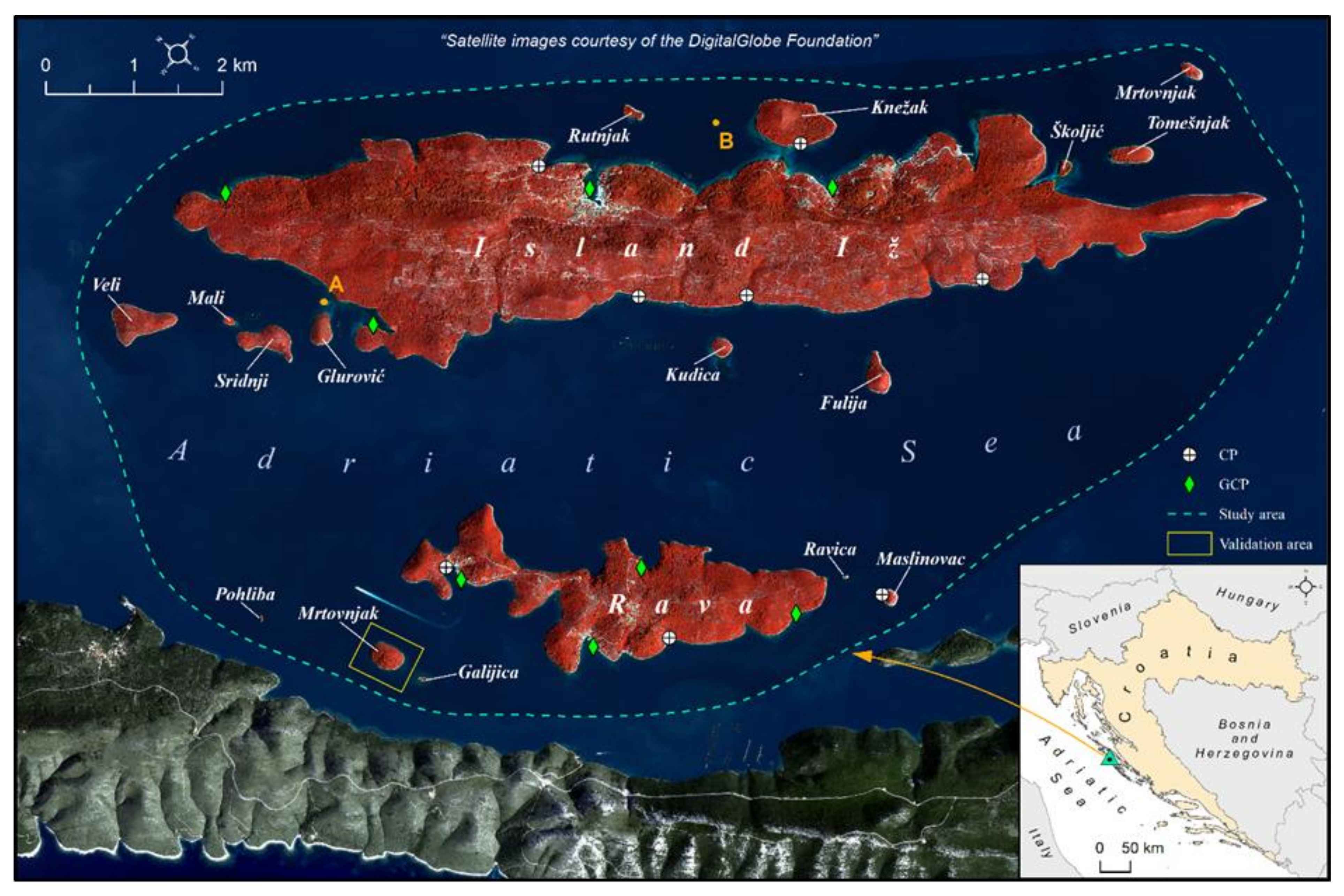
- determine the total number, area, and precise insular coastline length of all islands, islets, and rocks or rocks awash within the Iž-Rava island group using the automatic coastline mapping from WorldView2 (WV2)-derived models;
- (C)
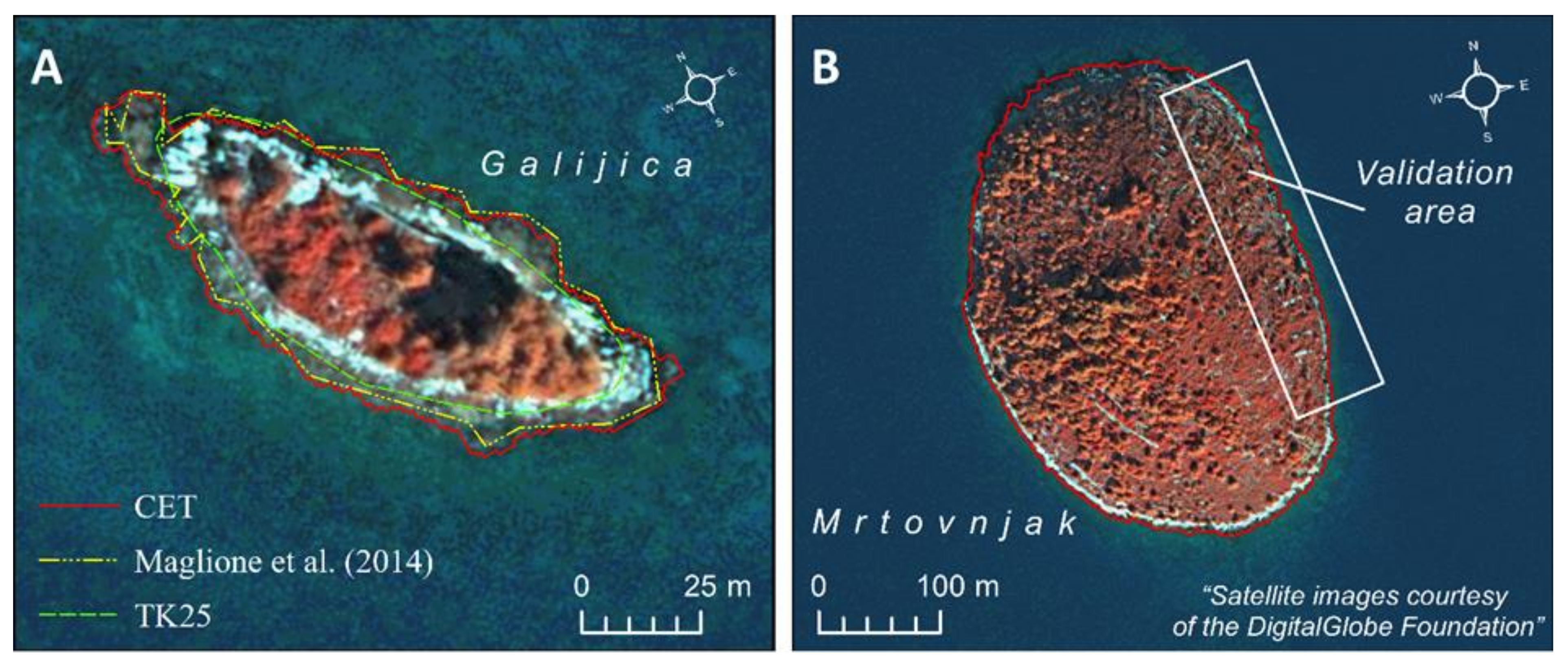
- validate the accuracy of coastline extraction from WV-derived imagery and DSM in comparison to field-collected reference data.
Study Area
2. Materials and Methods
2.1. WorldView-2 (WV2) Multispectral Imagery Preprocessing
2.2. Derivation of High-Resolution DSM from WV-2 Stereo-Pairs
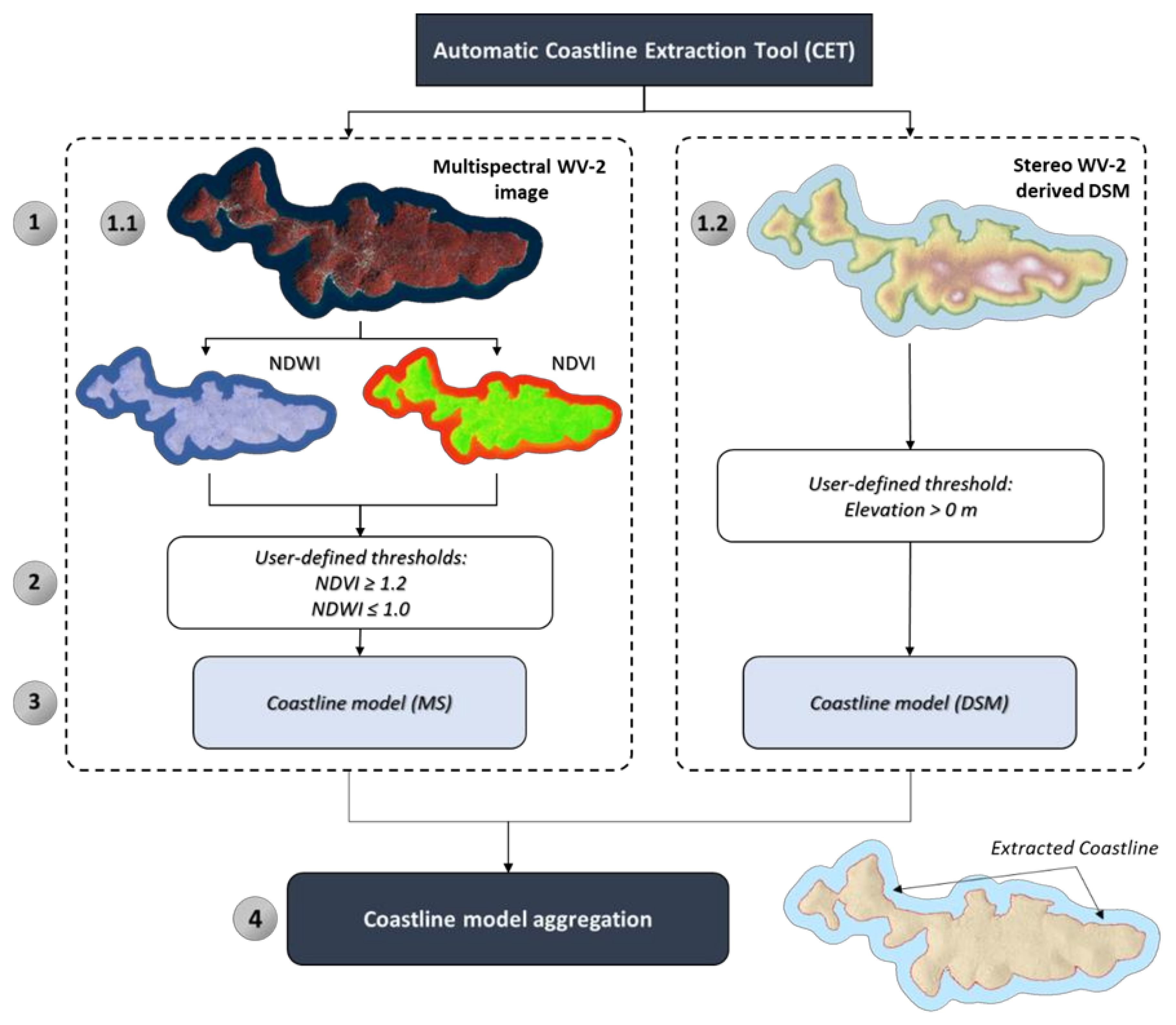
2.3. Development of Coastline Extration Tool (CET)
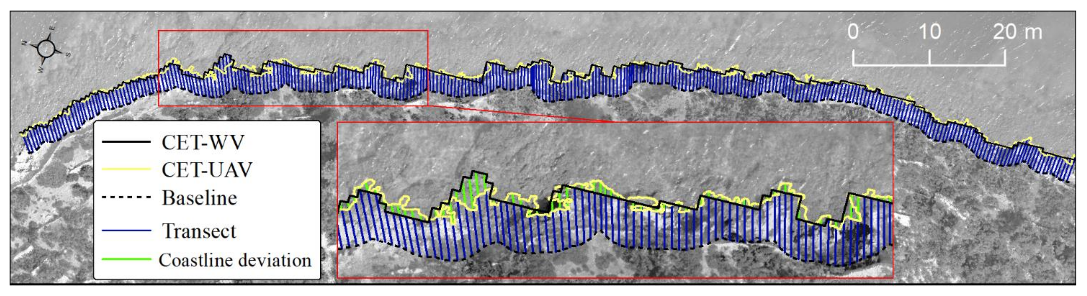
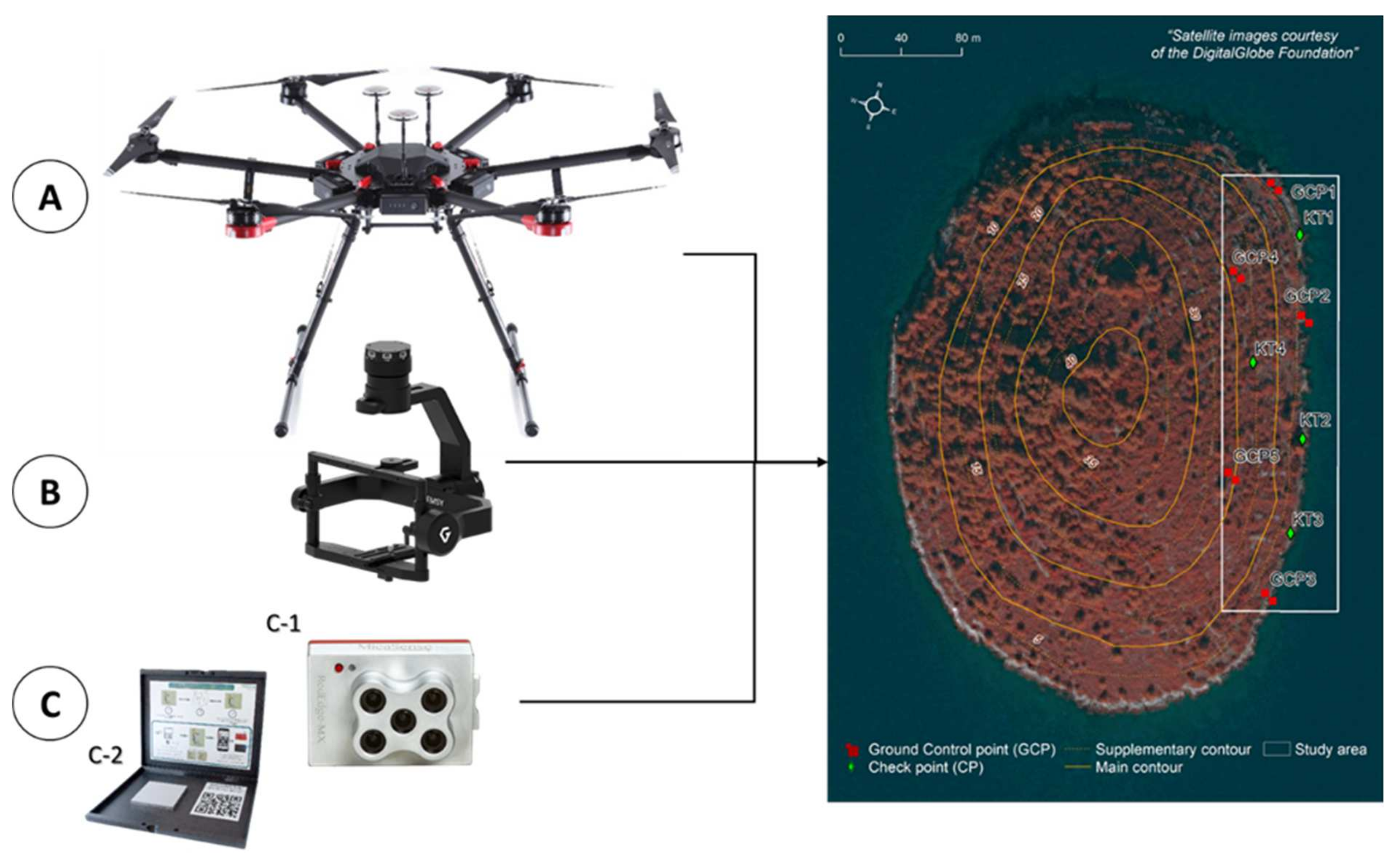
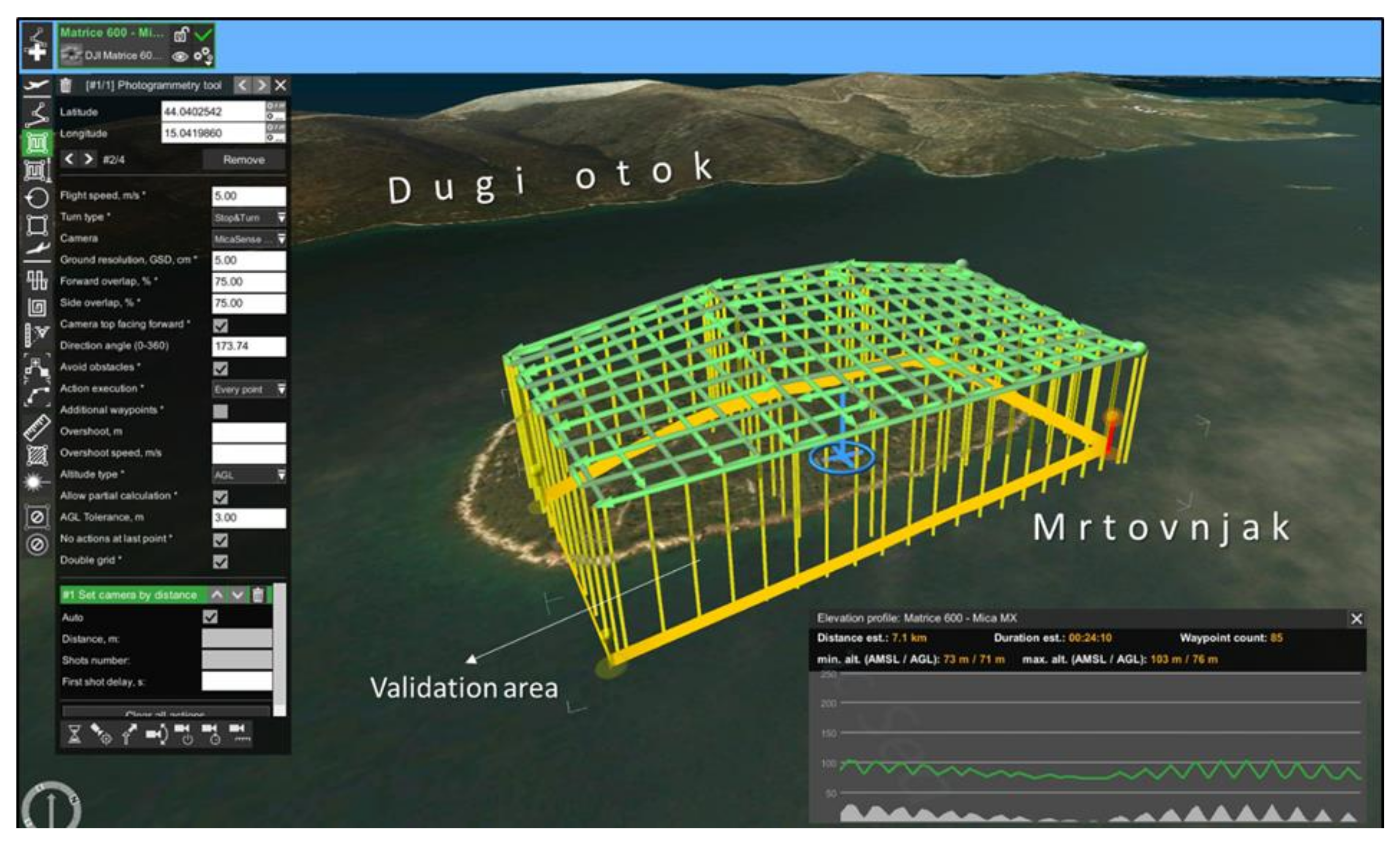
2.4. Field Acquisition and Processing of UAV Reference Data
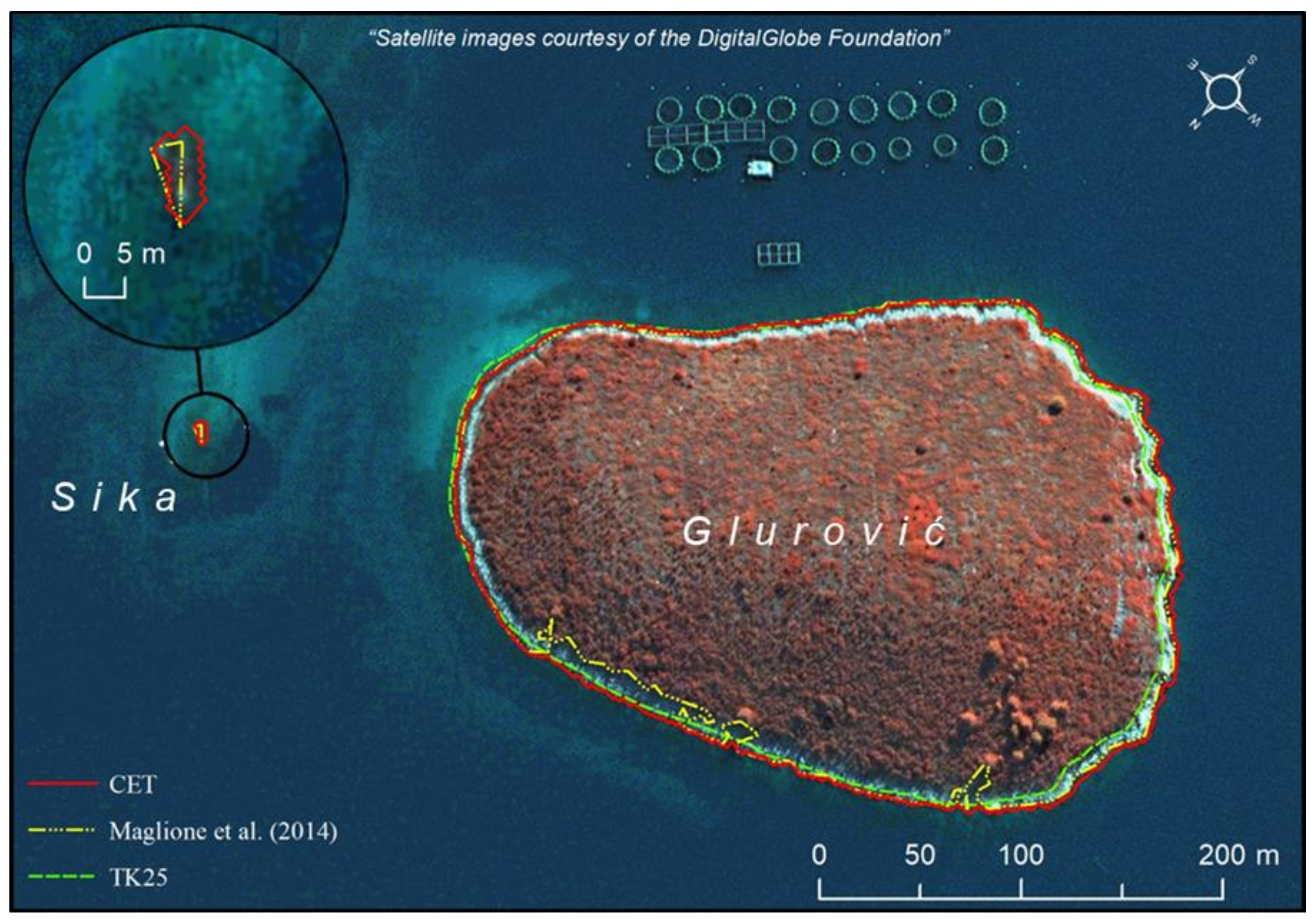
2.5. Extraction and Validation of CET-WV Coastlines
- (A)
- coastlines from the Topographic map of the Republic of Croatia (1:25,000);
- (B)
- coastlines derived from preprocessed multispectral WV-2 image (WV-MS) by a tool developed in [14].
3. Results
3.1. Results of CET Application on WV-Derived Models
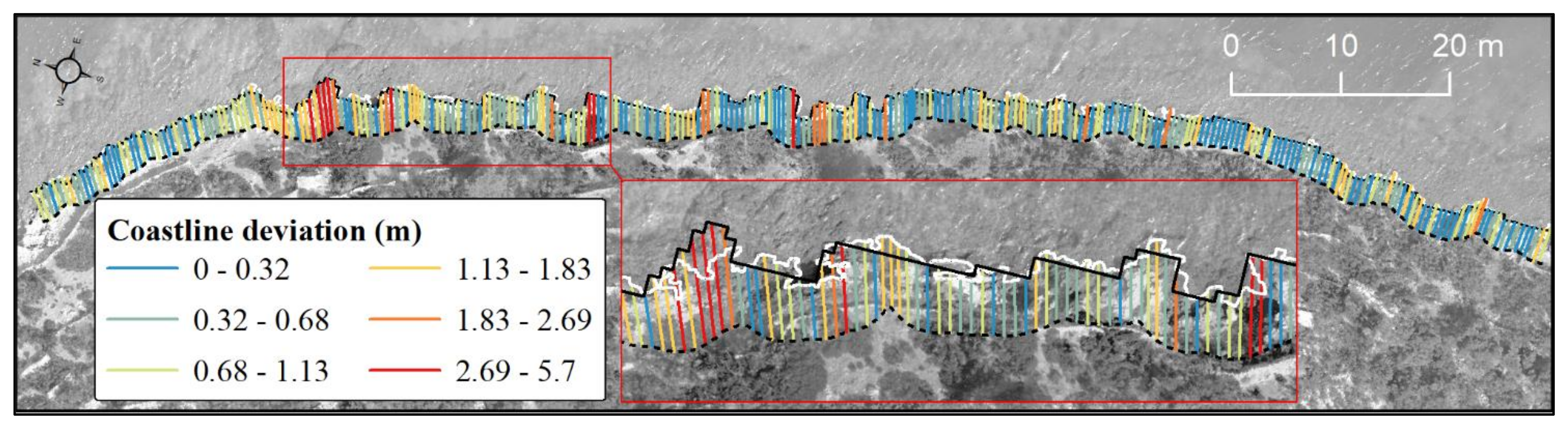
3.2. Validation of CET-WV-Extracted Coastline with Reference UAV Data
4. Discussion
4.1. Advantages of Developed CET
4.1.1. Detailed Coastline Mapping and Representation
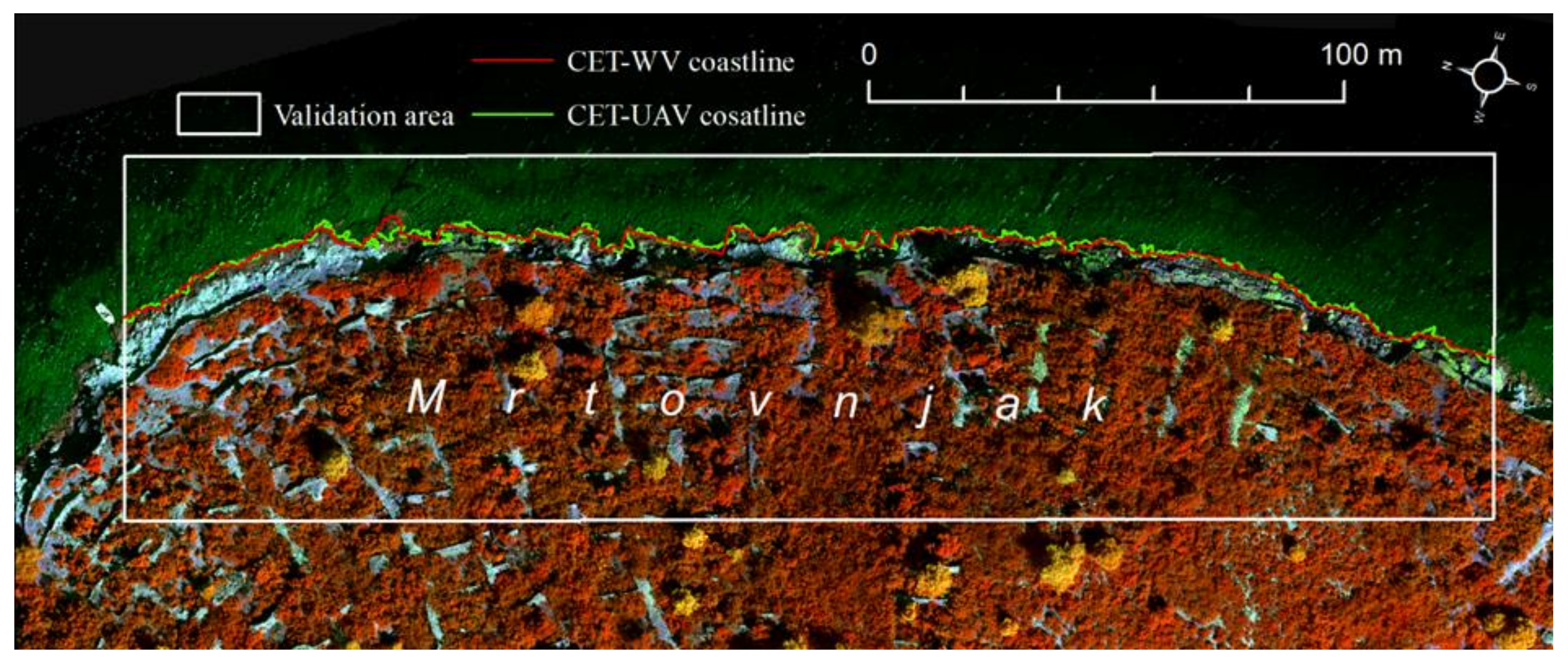
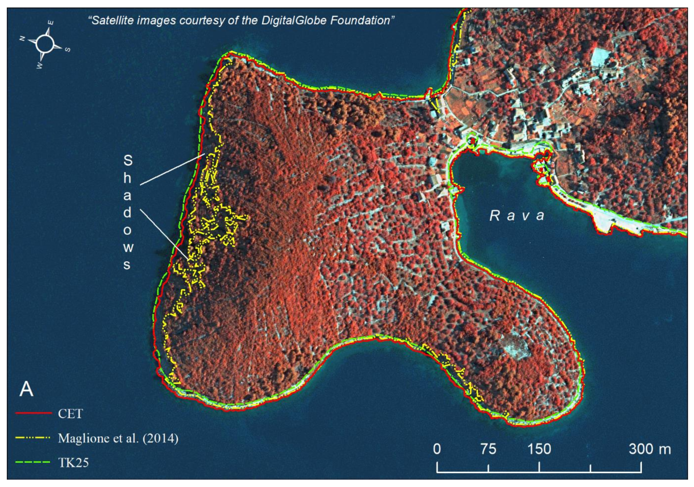
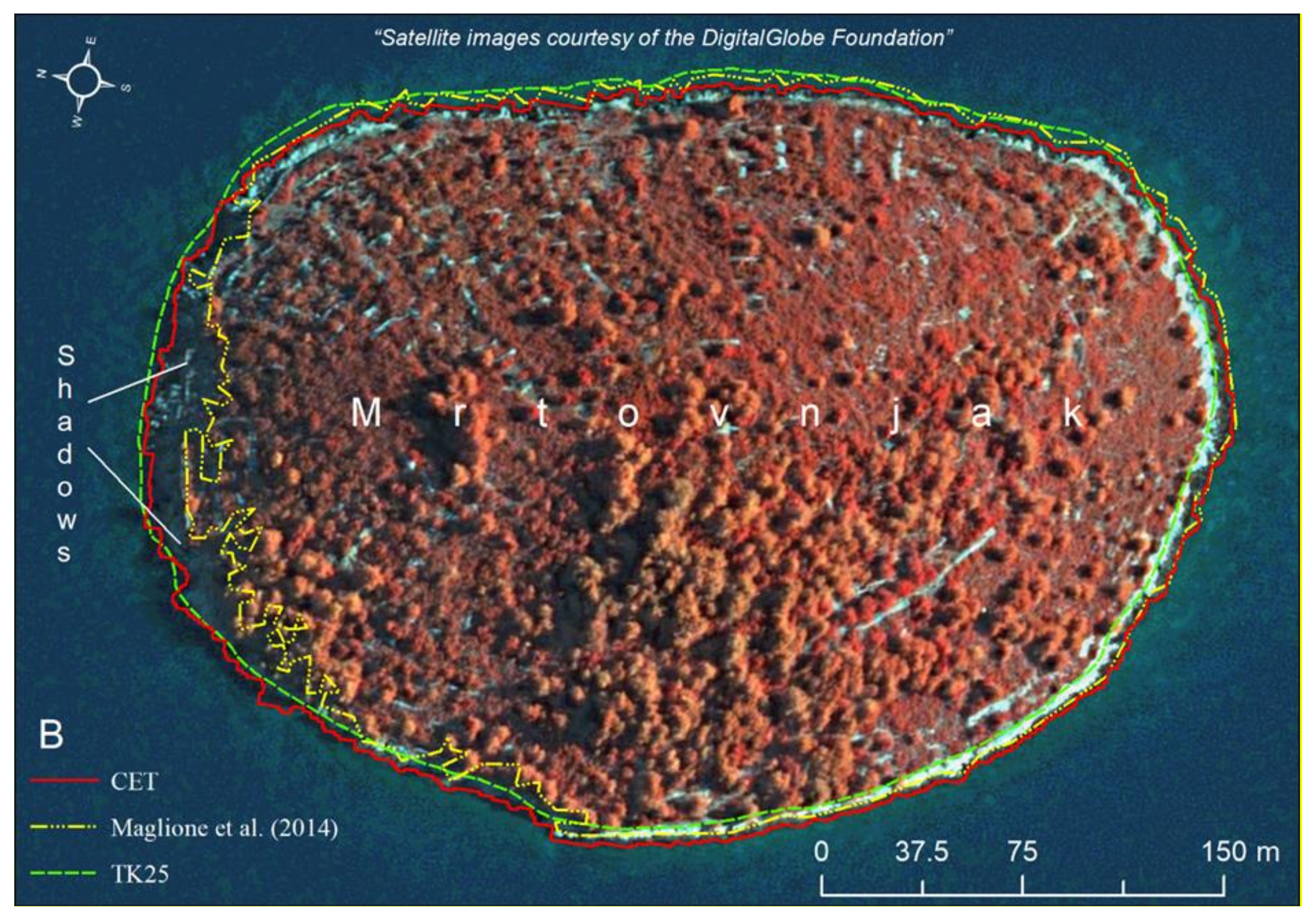
4.1.2. Elimination of Errors Caused by Shadows
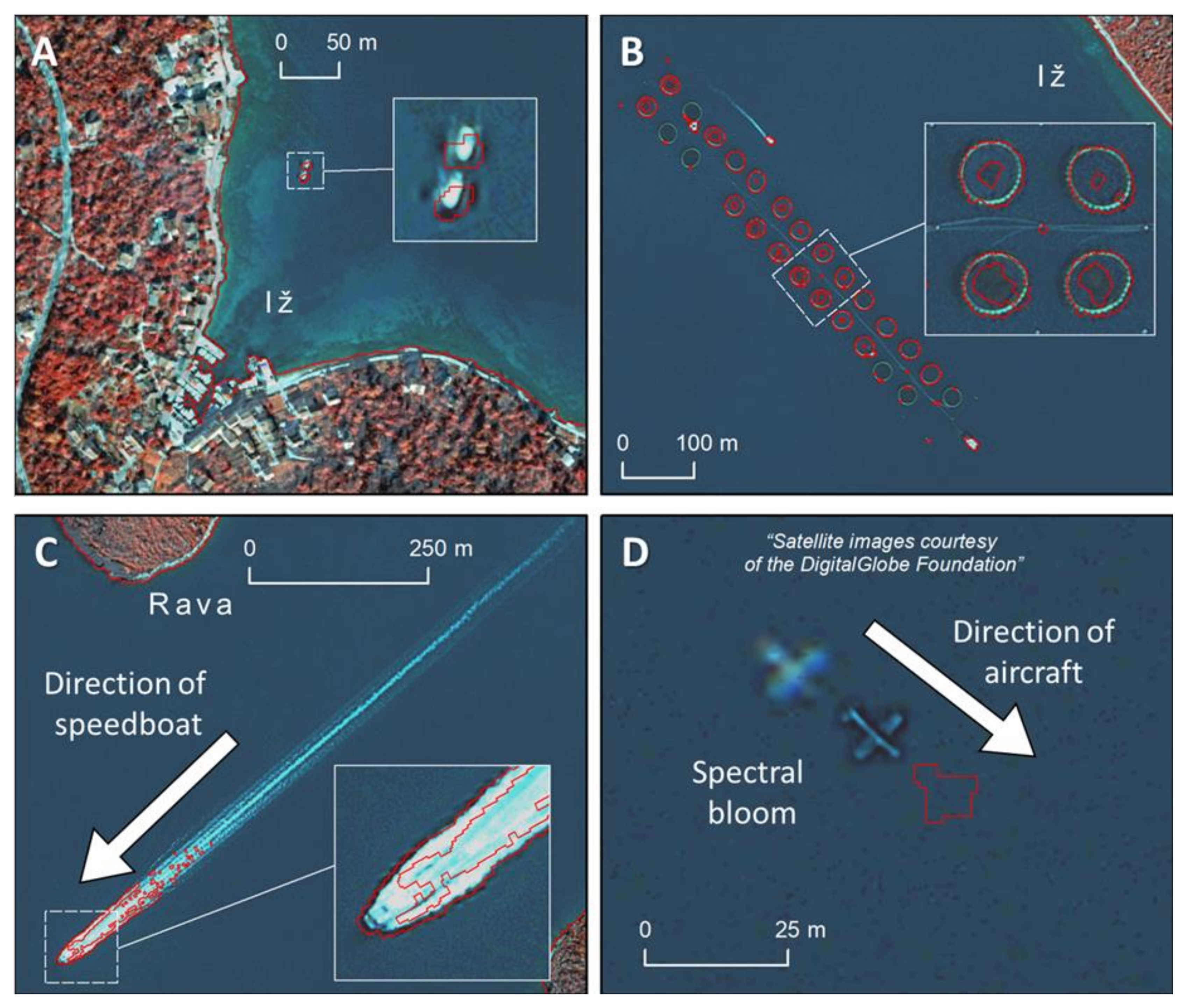
4.1.3. Wide Range of Other Potential Applications
4.1.4. Detection of Spatio-Temporal Changes in Coastline Position
4.1.5. Applicability of CET to Different Data Types
4.2. Limitation of the Developed CET
4.3. Future Upgrades of CET Tool
5. Conclusions
Supplementary Materials
Author Contributions
Funding
Institutional Review Board Statement
Informed Consent Statement
Data Availability Statement
Acknowledgments
Conflicts of Interest
References
- International Hydrographic Organization (IHO). Hydrographic Dictionary; International Hydrographic Organisation: Monaco, 1974; p. 216. [Google Scholar]
- Kuleli, T. Quantitative analysis of shoreline changes at the Mediterranean Coast in Turkey. Environ. Monit. Assess. 2009, 167, 387–397. [Google Scholar] [CrossRef] [PubMed]
- Martinez, M.L.; Taramelli, A.; Silva, R. Resistance and Resilience: Facing the Multidimensional Challenges in Coastal Areas. J. Coast. Res. 2017, 77, 1–6. [Google Scholar] [CrossRef]
- Kron, W. Coasts: The high-risk areas of the world. Nat. Hazards 2013, 66, 1363–1382. [Google Scholar] [CrossRef]
- Hinkel, J.; Lincke, D.; Vafeidis, A.; Perrette, M.; Nicholls, R.; Tol, R.; Marzeion, B.; Fettweis, X.; Ionescu, C.; Levermann, A. Coastal flood damage and adaptation costs under 21st century sea-level rise. Proc. Natl. Acad. Sci. USA 2014, 111, 3292–3297. [Google Scholar] [CrossRef] [Green Version]
- Simonovic, S.P.; Peck, A. Dynamic Resilience to Climate Change Caused Natural Disasters in Coastal Megacities Quantification Framework. Br. J. Environ. Clim. Chang. 2013, 3, 378–401. [Google Scholar] [CrossRef]
- Neumann, B.; Vafeidis, A.T.; Zimmermann, J.; Nicholls, R.J. Future coastal population growth and exposure to sea-level rise and coastal flooding-a global assessment. PloS ONE 2015, 10, e0118571. [Google Scholar] [CrossRef] [Green Version]
- United Nations. Factsheet: People and Oceans. In Proceedings of the Ocean Conference, New York, NY, USA, 5–6 June 2017. [Google Scholar]
- Schwartz, M. Encyclopedia of Coastal Science; Springer Science & Business Media: Dordrecht, The Netherlands, 2006. [Google Scholar]
- Boak, E.H.; Turner, I. Shoreline Definition and Detection: A Review. J. Coast. Res. 2005, 214, 688–703. [Google Scholar] [CrossRef] [Green Version]
- Li, R.; Liu, J.-K.; Felus, Y. Spatial Modeling and Analysis for Shoreline Change Detection and Coastal Erosion Monitoring. Mar. Geodesy 2001, 24, 1–12. [Google Scholar] [CrossRef]
- Sunder, S.; Ramsankaran, R.; Ramakrishnan, B. Inter-comparison of remote sensing sensing-based shoreline mapping techniques at different coastal stretches of India. Environ. Monit. Assess. 2017, 189, 290. [Google Scholar] [CrossRef]
- Roberts, J. What’s the Difference Between Coastline and Shoreline? Available online: https://medium.com/@jenniferroberts050_60595/whats-the-difference-between-coastline-and-shoreline-982fcebf3ada (accessed on 15 January 2020).
- Maglione, P.; Parente, C.; Vallario, A. Coastline extraction using high resolution WorldView-2 satellite imagery. Eur. J. Remote Sens. 2014, 47, 685–699. [Google Scholar] [CrossRef]
- Dai, C.; Howat, I.M.; Larour, E.; Husby, E. Coastline extraction from repeat high resolution satellite imagery. Remote Sens. Environ. 2019, 229, 260–270. [Google Scholar] [CrossRef]
- Zhu, Z.; Tang, Y.; Hu, J.; An, M. Coastline Extraction from High-Resolution Multispectral Images by Integrating Prior Edge Information With Active Contour Model. IEEE J. Sel. Top. Appl. Earth Obs. Remote Sens. 2019, 12, 4099–4109. [Google Scholar] [CrossRef]
- Viaña-Borja, S.P.; Ortega-Sánchez, M. Automatic Methodology to Detect the Coastline from Landsat Images with a New Water Index Assessed on Three Different Spanish Mediterranean Deltas. Remote Sens. 2019, 11, 2186. [Google Scholar] [CrossRef] [Green Version]
- Dolan, R.; Hayden, B.P.; May, P.; May, S. The reliability of shoreline change measurements from aerial photographs. Shore Beach 1980, 48, 22–29. [Google Scholar]
- Di, K.; Ma, R.; Li, R. A Comparative Study of Shoreline Mapping Techniques. Res. Monogr. GIS 2004, 53–60. [Google Scholar] [CrossRef]
- Shaw, J.B.; Wolinsky, M.A.; Paola, C.; Voller, V. An image-based method for shoreline mapping on complex coasts. Geophys. Res. Lett. 2008, 35. [Google Scholar] [CrossRef]
- Mills, J.P.; Buckley, S.J.; Mitchell, H.L.; Clarke, P.J.; Edwards, S.J. A geomatics data integration technique for coastal change monitoring. Earth Surf. Process. Landforms 2005, 30, 651–664. [Google Scholar] [CrossRef]
- Marfai, M.A.; Almohamad, H.; Dey, S.; Susanto, B.; King, L. Coastal dynamic and shoreline mapping: Multi-sources spatial data analysis in Semarang Indonesia. Environ. Monit. Assess. 2007, 142, 297–308. [Google Scholar] [CrossRef]
- Moore, L.J. Shoreline mapping techniques. J. Coastal Res. 2000, 16, 111–124. [Google Scholar]
- Alesheikh, A.A.; Ghorbanali, A.; Nouri, N. Coastline change detection using remote sensing. Int. J. Environ. Sci. Technol. 2007, 4, 61–66. [Google Scholar] [CrossRef] [Green Version]
- Sanchez, A.J.; Lobo, F.J.; Azor, A.; Bárcenas, P.; Fernández-Salas, L.M.; del Río, V.D.; Peña, J.V.P. Human-driven coastline changes in the Adra River deltaic system, southeast Spain. Geomorphology 2010, 119, 9–22. [Google Scholar] [CrossRef]
- Wang, X.; Liu, Y.; Ling, F.; Liu, Y.; Fang, F. Spatio-Temporal Change Detection of Ningbo Coastline Using Landsat Time-Series Images during 1976–2015. ISPRS Int. J. Geo-Inf. 2017, 6, 68. [Google Scholar] [CrossRef] [Green Version]
- Ghosh, M.K.; Kumar, L.; Roy, C. Monitoring the coastline change of Hatiya Island in Bangladesh using remote sensing techniques. ISPRS J. Photogramm. Remote Sens. 2015, 101, 137–144. [Google Scholar] [CrossRef]
- Nikolakopoulos, K.; Kyriou, A.; Koukouvelas, I.; Zygouri, V.; Apostolopoulos, D. Combination of Aerial, Satellite, and UAV Photogrammetry for Mapping the Diachronic Coastline Evolution: The Case of Lefkada Island. ISPRS Int. J. Geo-Inf. 2019, 8, 489. [Google Scholar] [CrossRef] [Green Version]
- Forgiarini, A.P.P.; De Figueiredo, S.A.; Calliari, L.J.; Goulart, E.S.; Marques, W.; Trombetta, T.B.; Oleinik, P.H.; Guimarães, R.C.; Arigony-Neto, J.; Salame, C.C. Quantifying the geomorphologic and urbanization influence on coastal retreat under sea level rise. Estuar. Coast. Shelf Sci. 2019, 230, 106437. [Google Scholar] [CrossRef]
- Zhang, L.; Ouyang, Z. Focusing on rapid urbanization areas can control the rapid loss of migratory water bird habitats in China. Glob. Ecol. Conserv. 2019, 20, e00801. [Google Scholar] [CrossRef]
- Ghoneim, E.; Mashaly, J.; Gamble, D.; Halls, J.; AbuBakr, M. Nile Delta exhibited a spatial reversal in the rates of shoreline retreat on the Rosetta promontory comparing pre- and post-beach protection. Geomorphology 2015, 228, 1–14. [Google Scholar] [CrossRef]
- Lymburner, L.; Bunting, P.; Lucas, R.; Scarth, P.; Alam, I.; Phillips, C.; Ticehurst, C.; Held, A. Mapping the multi-decadal mangrove dynamics of the Australian coastline. Remote Sens. Environ. 2020, 238, 111185. [Google Scholar] [CrossRef]
- Rangel-Buitrago, N.; Neal, W.J.; de Jonge, V.N. Risk assessment as tool for coastal erosion management. Ocean Coast. Manag. 2020, 186, 105099. [Google Scholar] [CrossRef]
- Di, K.; Ma, R.; Wang, J.; Li, R. Coastal mapping and change detection using high-resolution IKONOS satellite imagery. In Proceedings of the 2003 Annual National Conference on Digital Government Research, Boston, MA, USA, 18–21 May 2003; pp. 1–4. [Google Scholar]
- Sesli, F.A.; Karsli, F.; Colkesen, I.; Akyol, N. Monitoring the changing position of coastlines using aerial and satellite image data: An example from the eastern coast of Trabzon, Turkey. Environ. Monit. Assess. 2008, 153, 391–403. [Google Scholar] [CrossRef]
- Li, X.; Damen, M.C. Coastline change detection with satellite remote sensing for environmental management of the Pearl River Estuary, China. J. Mar. Syst. 2010, 82, S54–S61. [Google Scholar] [CrossRef]
- Dewi, R.S.; Bijker, W.; Stein, A.; Marfai, M.A. Fuzzy Classification for Shoreline Change Monitoring in a Part of the Northern Coastal Area of Java, Indonesia. Remote Sens. 2016, 8, 190. [Google Scholar] [CrossRef] [Green Version]
- Saleem, A.; Awange, J. Coastline shift analysis in data deficient regions: Exploiting the high spatio-temporal resolution Sentinel-2 products. Catena 2019, 179, 6–19. [Google Scholar] [CrossRef] [Green Version]
- Gens, R. Remote sensing of coastlines: Detection, extraction and monitoring. Int. J. Remote Sens. 2010, 31, 1819–1836. [Google Scholar] [CrossRef]
- Sammler, K.G. The rising politics of sea level: Demarcating territory in a vertically relative world. Territ. Politics Gov. 2020, 8, 604–620. [Google Scholar] [CrossRef]
- Stoa, R. The Coastline Paradox. Rutgers Univ. Law Rev. 2020, 72, 50. [Google Scholar] [CrossRef]
- Morton, R.A. Accurate shoreline mapping: Past, present, and future. In Coastal Sediments; American Society of Civil Engineers: New York, NY, USA, 1991; pp. 997–1010. [Google Scholar]
- Liu, Y.; Wang, X.; Ling, F.; Xu, S.; Wang, C. Analysis of Coastline Extraction from Landsat-8 OLI Imagery. Water 2017, 9, 816. [Google Scholar] [CrossRef] [Green Version]
- Niya, A.K.; Alesheikh, A.A.; Soltanpor, M.; Kheirkhahzarkesh, M.M. Shoreline change mapping using remote sensing and GIS. Inter. J. Remote Sens. Appl. 2013, 3, 102–107. [Google Scholar]
- Ding, Y.; Yang, X.; Jin, H.; Wang, Z.; Liu, Y.; Liu, B.; Zhang, J.; Liu, X.; Gao, K.; Meng, D. Monitoring Coastline Changes of the Malay Islands Based on Google Earth Engine and Dense Time-Series Remote Sensing Images. Remote Sens. 2021, 13, 3842. [Google Scholar] [CrossRef]
- Paravolidakis, V.; Ragia, L.; Moirogiorgou, K.; Zervakis, M.E. Automatic Coastline Extraction Using Edge Detection and Optimization Procedures. Geosciences 2018, 8, 407. [Google Scholar] [CrossRef] [Green Version]
- Guariglia, A.; Buonamassa, A.; Losurdo, A.; Saladino, R.; Trivigno, M.L.; Zaccagnino, A.; Colangelo, A. A multisource approach for coastline mapping and identification of shoreline changes. Ann. Geophys. 2009, 49, 295. [Google Scholar] [CrossRef]
- Guo, Q.; Pu, R.; Zhang, B.; Gao, L. A comparative study of coastline changes at Tampa Bay and Xiangshan Harbor during the last 30 years. In Proceedings of the 2016 IEEE International Geoscience and Remote Sensing Symposium (IGARSS), Beijing, China, 10–15 July 2016; pp. 5185–5188. [Google Scholar] [CrossRef]
- Zanutta, A.; Lambertini, A.; Vittuari, L. UAV Photogrammetry and Ground Surveys as a Mapping Tool for Quickly Monitoring Shoreline and Beach Changes. J. Mar. Sci. Eng. 2020, 8, 52. [Google Scholar] [CrossRef] [Green Version]
- Duplančić Leder, T.; Ujević, T.; Čala, M. Coastline lenghts and areas of islands in the croatian part of the Adriatic Sea determined from the topographic maps at the scale of 1: 25,000. Geoadria 2004, 9, 5–32. [Google Scholar]
- State Geodetic Administration of the Republic of Croatia. Data Catalog (Version 1.11). 2020. Available online: https://dgu.gov.hr/UserDocsImages//dokumenti/Pristup%20informacijama/Zakoni%20i%20ostali%20propisi/Ostalo//Katalog_podataka_DGU_2018_v11.pdf (accessed on 14 November 2020).
- Faričić, J. Geografija Sjevernodalmatinskih Otoka [Geography of North Dalmatian islands]; Školska Knjiga dd, Zadar Sveučilište u Zadru: Zagreb, Croatia, 2012. [Google Scholar]
- Pikelj, K.; Juračić, M. Eastern Adriatic Coast (EAC): Geomorphology and coastal vulnerability of a karstic coast. J. Coastal Res. 2013, 29, 944–957. [Google Scholar] [CrossRef]
- Digital Globe Foundation (DGF). Imagery Grant Application Process. 2019. Available online: http://www.digitalglobefoundation.org (accessed on 18 September 2019).
- Roa-Melgarejo, O.; Ariza, A.; Ramírez, H.M.; León-Rincón, H. Comparison of ATCOR Atmospheric and ELM Linear Empirical Correction Models Applied to WorldView-2 Images. Tecciencia 2018, 13, 29–38. [Google Scholar]
- Vermeulen, D.; van Niekerk, A. Evaluation of a WorldView-2 image for soil salinity monitoring in a moderately affected irrigated area. J. Appl. Remote Sens. 2016, 10, 1–32. [Google Scholar] [CrossRef]
- Madonsela, S.; Cho, M.A.; Mathieu, R.; Mutanga, O.; Ramoelo, A.; Kaszta, Ż.; Van De Kerchove, R.; Wolff, E. Multi-phenology WorldView-2 imagery improves remote sensing of savannah tree species. Int. J. Appl. Earth Obs. Geoinf. 2017, 58, 65–73. [Google Scholar] [CrossRef] [Green Version]
- Aguilar, M.A.; Novelli, A.; Nemamoui, A.; Aguilar, F.J.; Lorca, A.G.; González-Yebra, Ó. Optimizing Multiresolution Segmentation for Extracting Plastic Greenhouses from WorldView-3 Imagery. In Proceedings of the Handbook of Deep Learning Applications; Gabler: Vilamoura, Portugal, 2018; pp. 31–40. [Google Scholar]
- Li, H.; Jing, L.; Tang, Y. Assessment of Pansharpening Methods Applied to WorldView-2 Imagery Fusion. Sensors 2017, 17, 89. [Google Scholar] [CrossRef]
- Li, X.; He, M.; Zhang, L. Hyperspherical color transform based pansharpening method for WorldView-2 satellite images. In Proceedings of the 2013 IEEE 8th Conference on Industrial Electronics and Applications (ICIEA), Melbourne, Australia, 19–21 June 2013; pp. 520–523. [Google Scholar]
- Cheng, P.; Chaapel, C. Pan-sharpening and Geometric Correction: WorldView-2 Satellite. GeoInformatics 2010, 13, 30. [Google Scholar]
- Aguilar, M.A.; Saldaña, M.D.M.; Aguilar, F.J. Assessing geometric accuracy of the orthorectification process from GeoEye-1 and WorldView-2 panchromatic images. Int. J. Appl. Earth Obs. Geoinf. 2013, 21, 427–435. [Google Scholar] [CrossRef]
- ESRI. Overview of Georeferencing. Available online: https://pro.arcgis.com/en/pro-app/help/data/imagery/overview-of-georeferencing.htm (accessed on 23 May 2021).
- Jain, K.; Ravibabu, M.V.; Shafi, J.A.; Singh, S.P. Using rational polynomial coefficients (RPC) to generate digital elevation models—A comparative study. Appl. GIS 2009, 5, 1–11. [Google Scholar]
- Goldbergs, G.; Maier, S.W.; Levick, S.R.; Edwards, A. Limitations of high resolution satellite stereo imagery for estimating canopy height in Australian tropical savannas. Int. J. Appl. Earth Obs. Geoinf. 2019, 75, 83–95. [Google Scholar] [CrossRef]
- Domazetović, F.; Šiljeg, A.; Marić, I.; Jurišić, M. Assessing the Vertical Accuracy of Worldview-3 Stereo-extracted Digital Surface Model over Olive Groves. In Proceedings of the 6th International Conference on Geographical Information Systems Theory, Applications and Management, Prague, Czech Republic, 7–9 May 2020; pp. 246–253. [Google Scholar]
- DJI. MATRICE 600 PROSpecs. 2020. Available online: https://www.dji.com/hr/matrice600-pro/info#specs (accessed on 15 November 2020).
- MicaSense. RedEdge MX—The Sensor That Doesn’t Compromise. 2020. Available online: https://micasense.com/rededge-mx/ (accessed on 15 November 2020).
- James, M.R.; Chandler, J.H.; Eltner, A.; Fraser, C.; Miller, P.E.; Mills, J.P.; Lane, S.N. Guidelines on the use of structure-from-motion photogrammetry in geomorphic research. Ear. Sur. Proc. Land. 2019, 44, 2081–2084. [Google Scholar] [CrossRef]
- Hexagon. Extract Coastline from WorldView-2 & -3 Satellite Imagery. 2020. Available online: https://community.hexagongeospatial.com/t5/Spatial-Modeler-Tutorials/Extract-Coastline-from-WorldView-2-amp-3-satellite-imagery/ta-p/27448 (accessed on 5 March 2020).
- Himmelstoss, E.A.; Henderson, R.E.; Kratzmann, M.G.; Farris, A.S. Digital Shoreline Analysis System (DSAS) Version 5.0 User Guide; Open-File Report 2018-1179; USGS: Reston, VA, USA, 2018. [Google Scholar]
- Tsokos, A.; Kotsi, E.; Petrakis, S.; Vassilakis, E. Combining series of multi-source high spatial resolution remote sensing datasets for the detection of shoreline displacement rates and the effectiveness of coastal zone protection measures. J. Coast. Conserv. 2018, 22, 431–441. [Google Scholar] [CrossRef]
- Heiselberg, H. Aircraft and Ship Velocity Determination in Sentinel-2 Multispectral Images. Sensors 2019, 19, 2873. [Google Scholar] [CrossRef] [PubMed] [Green Version]
- Nagarajan, S.; Khamaru, S.; De Witt, P. UAS based 3D shoreline change detection of Jupiter Inlet Lighthouse ONA after Hurricane Irma. Int. J. Remote Sens. 2019, 40, 9140–9158. [Google Scholar] [CrossRef]
- Corbane, C.; Najman, L.; Pecoul, E.; Demagistri, L.; Petit, M. A complete processing chain for ship detection using optical satellite imagery. Int. J. Remote Sens. 2010, 31, 5837–5854. [Google Scholar] [CrossRef]
- Gianinetto, M.; Aiello, M.; Marchesi, A.; Topputo, F.; Massari, M.; Lombardi, R.; Banda, F.; Tebaldini, S. OBIA ship detection with multispectral and SAR images: A simulation for Copernicus security applications. In Proceedings of the 2016 IEEE International Geoscience and Remote Sensing Symposium (IGARSS), Beijing, China, 10–15 July 2016; pp. 1229–1232. [Google Scholar]
- Kanjir, U. Detecting migrant vessels in the Mediterranean Sea: Using Sentinel-2 images to aid humanitarian actions. Acta Astronaut. 2019, 155, 45–50. [Google Scholar] [CrossRef]
- Kurekin, A.A.; Loveday, B.R.; Clements, O.; Quartly, G.D.; Miller, P.I.; Wiafe, G.; Agyekum, K.A. Operational Monitoring of Illegal Fishing in Ghana through Exploitation of Satellite Earth Observation and AIS Data. Remote Sens. 2019, 11, 293. [Google Scholar] [CrossRef] [Green Version]
- Maxar. Worldview-2. Datasheet. 2020. Available online: https://www.maxar.com/constellation (accessed on 12 November 2020).
- Handcock, R.N.; Torgersen, C.E.; Cherkauer, K.A.; Gillespie, A.R.; Tockner, K.; Faux, R.N.; Tan, J. Thermal Infrared Remote Sensing of Water Temperature in Riverine Landscapes. Fluv. Remote Sens. Sci. Manag. 2012, 1, 85–113. [Google Scholar] [CrossRef]
- Ghorai, D.; Mahapatra, M. Extracting Shoreline from Satellite Imagery for GIS Analysis. Remote Sens. Ear. Syst. Sci. 2020, 3, 1–10. [Google Scholar] [CrossRef]
- Lega, M.; Napoli, R.M.A. Aerial infrared thermography in the surface waters contamination monitoring. Desalination Water Treat. 2010, 23, 141–151. [Google Scholar] [CrossRef]
- DJI. Zenmuse XT2—User Manual 1.0. 2018. Available online: https://www.dji.com/hr/downloads/products/zenmuse-xt2 (accessed on 19 January 2021).


| Case Study (Authors) | Coastline Extraction Method Type | Study Area (km2) | Input Data | Limitations |
|---|---|---|---|---|
| [24] | Semiautomatic (histogram threshold/ frequency band ratio) | 5100 | Low-resolution imagery (Thematic Mapper (TM); Enhanced Thematic Mapper (ETM)) | Not applicable for large scale mapping [44] |
| [14] | Semiautomatic (maximum likelihood method) | Few km2 | High-resolution imagery (WorldView multispectral Imagery) | Not applicable for large scale mapping [44]; Based only on spectral information |
| [46] | Semiautomatic (edge detection operators) | Few km2 | High-resolution imagery (Aerial Images/WorldView multispectral imagery) | Not applicable for large scale mapping [44]; Based only on spectral information |
| [12] | Semiautomatic (adaptive thresholding) | Several hundred km2 | Low-resolution imagery (Landsat 8 OLI) | Based only on spectral information |
| [15] | Semiautomatic (adaptive thresholding) | Several thousand km2 | High-resolution imagery (Geoeye-1/Quickbird/WorldView) | Based only on spectral information |
| [16] | Semiautomatic (edge detection operators) | Few km2 | High-resolution imagery (GF1/GF2/Quickbird/ZY3) | Based only on spectral information |
| [17] | Semiautomatic (adaptive thresholding) | Few km2 | Low-resolution imagery (Landsat TM, ETM+, OLI) | Based only on spectral information |
| [45] | Semiautomatic (adaptive thresholding (edge detection)) | Several thousand km2 | Low-resolution imagery (Landsat) | Based only on spectral information |
| Point Type | No | RMSE X (m) | RMSE Y (m) | RMSE Z (m) | MEAN RMSE (m) |
|---|---|---|---|---|---|
| GCP | 8 | 0.403 | 0.684 | 0.484 | 0.524 |
| CP | 8 | 0.398 | 0.751 | 0.749 | 0.633 |
| TP | 159 | 0.063 | 0.016 | 0.013 | 0.031 |
| Parameter | User-Defined Settings | Point Type | Total RMSE (cm) |
|---|---|---|---|
| Alignment parameters | Accuracy: High | Control points | 9.68 |
| Generic preselection: Yes | |||
| Reference preselection: Yes | |||
| Key point limit: 40,000 | |||
| Tie point limit: 10,000 | |||
| Dense point cloud: reconstruction parameters | Quality: High | Check points | 10.29 |
| Filtering mode: Aggressive |
| ID | Island Name | Coastline Length (m) | ||
|---|---|---|---|---|
| TM (1:25,000) | [14] | CET-WV | ||
| 1 | Iž | 36,546.77 | 44,461.74 | 49,754.00 |
| 2 | Rava | 16,662.97 | 23,765.53 | 22,512.00 |
| 3 | Knežak | 2415.48 | 3146.12 | 3310.00 |
| 4 | Beli | 1996.52 | 2182.22 | 2678.00 |
| 5 | Sridnji | 1800.95 | 2124.16 | 2406.00 |
| 6 | Fulija | 1239.08 | 1761.92 | 1688.00 |
| 7 | Tomešnjak | 1192.04 | 1423.79 | 1514.00 |
| 8 | Mrtovnjak (Rava) | 1108.53 | 1578.99 | 1660.00 |
| 9 | Glurović | 997.55 | 1225.01 | 1372.00 |
| 10 | Mrtovnjak (Iž) | 707.59 | 899.98 | 944.00 |
| 11 | Kudica | 691.41 | 745.22 | 932.00 |
| 12 | Rutnjak | 681.47 | 898.27 | 774.00 |
| 13 | Maslinovac | 592.10 | 628.07 | 908.00 |
| 14 | Školjić | 536.58 | 730.71 | 762.00 |
| 15 | Mali | 376.20 | 411.62 | 520.00 |
| 16 | Galijica | 248.14 | 345.45 | 416.00 |
| 17 | Pohliba | 177.19 | 244.80 | 302.00 |
| 18 | Ravica | 173.11 | 215.63 | 258.00 |
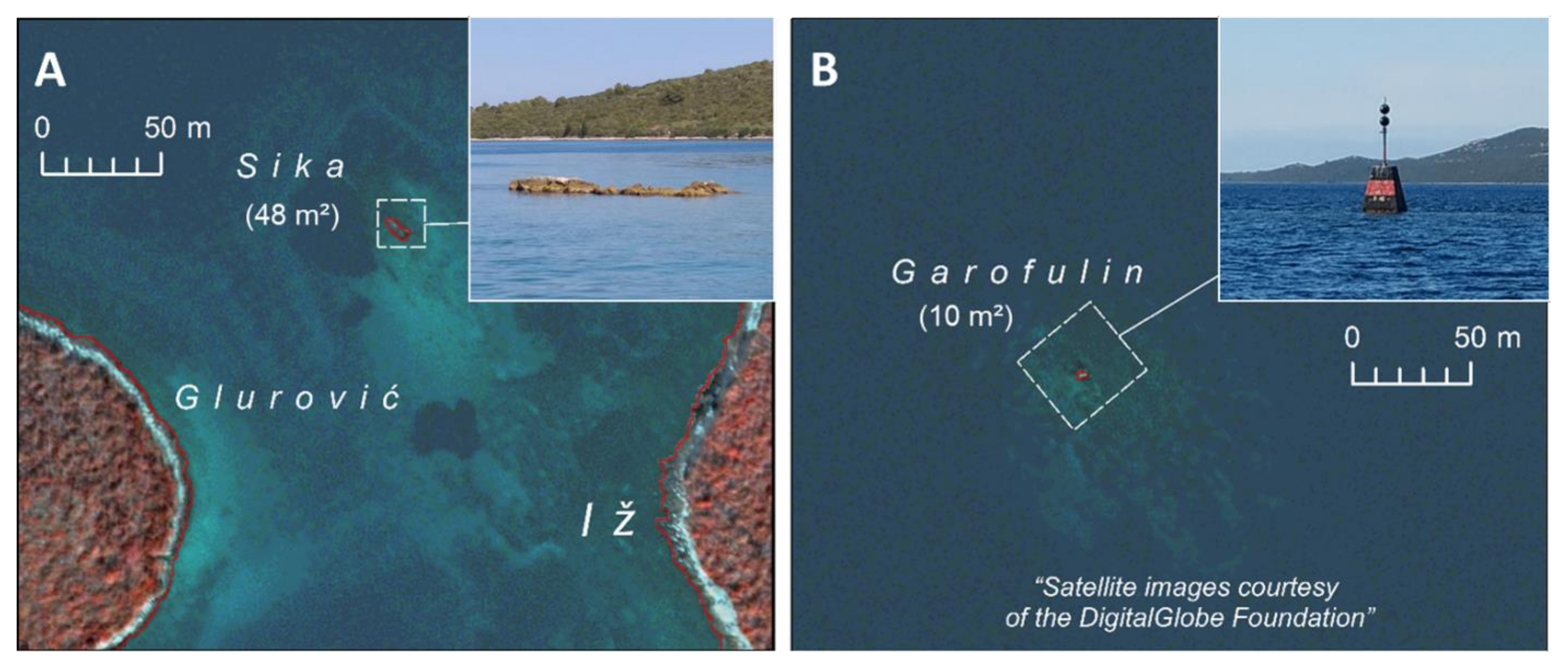
| 19 | Sika | - | 24.99 | 38.00 |
| 20 | Garofulin | - | 9.72 | 14.00 |
| Total coastline length (m) | 68,143.67 | 86,823.93 | 92,762.00 | |
| ID | Island Name | Total Area (ha) | Total Area (km2) | ||||
|---|---|---|---|---|---|---|---|
| TM (1:25,000) | [14] | CET-WV | TM (1:25,000) | [14] | CET-WV | ||
| 1 | Iž | 1655.48 | 1658.08 | 1662.25 | 16.555 | 16.581 | 16.622 |
| 2 | Rava | 363.76 | 360.83 | 367.93 | 3.638 | 3.608 | 3.679 |
| 3 | Knežak | 36.78 | 36.33 | 36.90 | 0.368 | 0.363 | 0.369 |
| 4 | Beli | 20.04 | 20.32 | 20.40 | 0.200 | 0.203 | 0.204 |
| 5 | Sridnji | 13.76 | 14.16 | 14.35 | 0.138 | 0.142 | 0.143 |
| 6 | Fulija | 9.03 | 8.85 | 9.28 | 0.090 | 0.089 | 0.093 |
| 7 | Tomešnjak | 8.98 | 8.21 | 9.12 | 0.083 | 0.082 | 0.091 |
| 8 | Mrtovnjak (Rava) | 8.32 | 8.72 | 8.33 | 0.090 | 0.087 | 0.083 |
| 9 | Glurović | 6.85 | 6.91 | 7.11 | 0.068 | 0.069 | 0.071 |
| 10 | Mrtovnjak (Iž) | 3.69 | 3.30 | 3.95 | 0.033 | 0.033 | 0.040 |
| 11 | Kudica | 3.32 | 3.93 | 3.40 | 0.037 | 0.039 | 0.034 |
| 12 | Rutnjak | 2.69 | 2.51 | 2.72 | 0.027 | 0.025 | 0.027 |
| 13 | Maslinovac | 2.44 | 2.66 | 2.65 | 0.0244 | 0.0266 | 0.0265 |
| 14 | Školjić | 2.03 | 2.02 | 2.17 | 0.0203 | 0.0202 | 0.0217 |
| 15 | Mali | 0.97 | 1.07 | 1.10 | 0.0097 | 0.0107 | 0.0110 |
| 16 | Galijica | 0.33 | 0.42 | 0.44 | 0.0033 | 0.0042 | 0.0044 |
| 17 | Pohliba | 0.18 | 0.17 | 0.27 | 0.0018 | 0.0017 | 0.0027 |
| 18 | Ravica | 0.17 | 0.21 | 0.23 | 0.0017 | 0.0021 | 0.0023 |
| 19 | Sika | - | 0.002 | 0.005 | - | 0.000020 | 0.000048 |
| 20 | Garofulin | - | 0.0004 | 0.0010 | - | 0.000004 | 0.000010 |
| Total area | 2138.81 | 2138.71 | 2152.60 | 21.388 | 21.387 | 21.526 | |
Publisher’s Note: MDPI stays neutral with regard to jurisdictional claims in published maps and institutional affiliations. |
© 2021 by the authors. Licensee MDPI, Basel, Switzerland. This article is an open access article distributed under the terms and conditions of the Creative Commons Attribution (CC BY) license (https://creativecommons.org/licenses/by/4.0/).
Share and Cite
Domazetović, F.; Šiljeg, A.; Marić, I.; Faričić, J.; Vassilakis, E.; Panđa, L. Automated Coastline Extraction Using the Very High Resolution WorldView (WV) Satellite Imagery and Developed Coastline Extraction Tool (CET). Appl. Sci. 2021, 11, 9482. https://doi.org/10.3390/app11209482
Domazetović F, Šiljeg A, Marić I, Faričić J, Vassilakis E, Panđa L. Automated Coastline Extraction Using the Very High Resolution WorldView (WV) Satellite Imagery and Developed Coastline Extraction Tool (CET). Applied Sciences. 2021; 11(20):9482. https://doi.org/10.3390/app11209482
Chicago/Turabian StyleDomazetović, Fran, Ante Šiljeg, Ivan Marić, Josip Faričić, Emmanuel Vassilakis, and Lovre Panđa. 2021. "Automated Coastline Extraction Using the Very High Resolution WorldView (WV) Satellite Imagery and Developed Coastline Extraction Tool (CET)" Applied Sciences 11, no. 20: 9482. https://doi.org/10.3390/app11209482
APA StyleDomazetović, F., Šiljeg, A., Marić, I., Faričić, J., Vassilakis, E., & Panđa, L. (2021). Automated Coastline Extraction Using the Very High Resolution WorldView (WV) Satellite Imagery and Developed Coastline Extraction Tool (CET). Applied Sciences, 11(20), 9482. https://doi.org/10.3390/app11209482