Abstract
Model-based 3D/2D image registration using single-plane fluoroscopy is a common setup to determine knee joint kinematics, owing to its markerless aspect. However, the approach was subjected to lower accuracies in the determination of out-of-plane motion components. Introducing additional kinematic constraints with an appropriate anatomical representation may help ameliorate the reduced accuracy of single-plane image registration. Therefore, this study aimed to develop and evaluate a multibody model-based tracking (MbMBT) scheme, embedding a personalized kinematic model of the tibiofemoral joint for the measurement of tibiofemoral kinematics. The kinematic model was consisted of three ligaments and an articular contact mechanism. The knee joint activities in six volunteers during isolated knee flexion, lunging, and sit-to-stand motions were recorded with a biplane X-ray imaging system. The tibiofemoral kinematics determined with the MbMBT and mediolateral view fluoroscopic images were compared against those determined using biplane fluoroscopic images. The MbMBT was demonstrated to yield tibiofemoral kinematics with precision values in the range from 0.1 mm to 1.1 mm for translations and from 0.2° to 1.3° for rotations. The constraints provided by the kinematic model were shown to effectively amend the nonphysiological tibiofemoral motion and not compromise the image registration accuracy with the proposed MbMBT scheme.
1. Introduction
Accurate measurement of the three-dimensional motion and arthrokinematics of the knee is essential for the functional assessment of the joint. To this end, skin marker-based stereophotogrammetry is commonly used to measure the spatial poses of the thigh and shank. However, the soft tissue artifacts associated with skin markers inevitably reduced the accuracies of the measured tibiofemoral kinematics [1,2]. Appropriate kinematic models, either at the segment level [3] or at the multibody level [4], can be applied with the measured skin markers to better reproduce the spatial poses of the body segment of interest and thereafter more accurately estimate joint angles. Multibody kinematics optimization techniques require the kinematic model of the knee to strictly or loosely link the adjacent segments while providing constraints to unphysiological motions [5].
Various knee joint kinematics models were introduced and embedded into the multibody model with the intent of generating more accurate kinematics of the knee [6]. Among them, the spherical [4,7] and hinge models [8,9], the most simplified and commonly utilized in multibody kinematics optimization, were demonstrated to not enable physiological knee kinematics [6]. While the elastic knee model with a joint stiffness matrix showed the potential to better reproduce physiological kinematics [10], subject-specific customization of such stiffness coefficients should be further addressed. The spatial parallel mechanism represented by rigid links connecting adjacent joint articular surfaces is one of the most popular models in the community [6,11,12,13,14]. The approach was featured by its direct connection with anatomical structures (i.e., the ligaments and articular contacts) and capability to customize to individual subjects and replicate joint passive motion [15]. Recent studies have shown that the knee model based on a spatial parallel mechanism can be personalized by using personal medical images and 3D kinematics data [16,17]. Accurate representation of knee articular features has shown its potential to drive accurate 3D knee joint kinematics during non-weight-bearing knee flexion and extension motions with submillimeter and subdegree errors [17]. However, the feasibility of replicating accurate knee kinematics during various weight-bearing activities using the precise knee model remains unclear.
Model-based tracking (MBT) techniques integrating the dynamic X-ray imaging system, computed tomography (CT), and 3D/2D image registration methods [18,19,20,21] enabled direct measurement of 3D skeletal kinematics while eliminating the use of skin markers. The 3D pose of a skeleton can be determined by registering its CT model-projected digitally reconstructed radiographs (DRRs) to the X-ray images. The biplane imaging configuration is currently the most commonly used setup to capture the 3D movement of a single joint during particular tasks [22,23,24], as it can provide stereo X-ray images for 3D/2D image registration. The limited intersection volume of measurement and the higher ionizing radiation dose were considered the primary concerns of biplane configuration. While the application of a single-plane imaging system can enlarge the area of measurement (given the same size of the X-ray detector) and lead to lower radiation exposure to subjects, limited measurement accuracy was observed, especially in out-of-plane motion components [25,26,27,28]. This was associated with both the substantial differences between the DRRs and the X-ray images [29] and the perspective projection of the imaging system. The out-of-plane motion of a 3D bone model would have less influence on the appearance of the DRR and thus the objective function values than those by the in-plane motion components [28].
Introducing additional information other than the images during 3D/2D image registration may help ameliorate the reduced accuracy of single-plane image registration. For the analysis of the total knee replacement kinematics, the anti-collision maneuver was introduced to detect the unrealistic penetration between the metal and insert components, which was shown to yield more accurate relative poses between the femoral and tibial components in the out-of-plane translation component [30]. A similar maneuver was also applied on the vertebrae and shown to successfully increase the accuracy of intervertebral motion measurement [31]. However, anticollision detection may not be applicable to the natural knee, as the femur and tibia are not compactly close to each other. Instead, a personalized model with an appropriate representation of anatomical structures may provide useful information that helps guide the motion pattern of the tibiofemoral joint. Personalization of the knee model in vivo is a challenge, as the model parameters were demonstrated to have substantial influences on the model-determined kinematics [32]. Taking magnetic resonance (MR) images is a feasible approach to customize the model parameters [17], but it requires subjects to undergo additional MR scanning and be subjected to intra- and interobserver variability in identifying ligament attachment sites [33]. A feasible alternative is to use a generic digital model embedding known model parameters [34,35]. Personalization of model parameters can be thereafter obtained by proper nonrigid shape transform of the generic model to best-fit available anatomical features of the subject under analysis. The approach can be particularly suitable for the scenario of MBT, as 3D surface bone models are normally obtained from the subject’s CT. Since the knee model has the ability to guide the particular motion pattern given the subject-specific model parameters, properly integrating it with the image registration procedure may be beneficial to improve the accuracy of out-of-plane motion components.
The purpose of the present study was to develop a multibody model-based tracking (MbMBT) scheme based on simultaneous 3D/2D image registration of the femoral and tibial bones while considering the kinematic constraints provided by the personalized kinematic model of the tibiofemoral joint. To evaluate the performance of the proposed method, the reconstructed tibiofemoral kinematics of six young volunteers during functional tasks with the MbMBT approach were compared against those determined using a validated biplane MBT technique.
2. Materials and Methods
2.1. Imaging Acquisition
Six healthy male volunteers (age: 23.2 ± 1.7 years; mass: 74.2 ± 15.4 kg; height: 175.2 ± 4.2 cm) participated in this study. Prior to data acquisition, all subjects provided written informed consent, and the study was approved by the China Medical University and Hospital Research Ethics Committee. Computed tomography image stacks of the knee of all subjects (voxel size: 0.7 mm × 0.7 mm × 0.6 mm) were acquired from CT scans (Optima CT 660; GE Healthcare, Chicago, IL, USA). Semimanual segmentation with a region-growing algorithm was employed to isolate regions of the right femur and tibia/fibula, which were further used to create volumetric and surface bone models [21]. A clinical biplane X-ray imaging system (Allura Xper FD20/20, Philips Medical Systems, Amsterdam, The Netherlands) was set up with two X-ray units placed orthogonal to each other, from which medial-lateral (ML) and anterior-posterior (AP) view fluoroscopic images of an individual subject’s right knee during tested activities were acquired (resolution: 512 × 512; grayscale: 8 bit). The imaging system was operated at tube voltages ranging from 50 to 59 kVp, a tube current of 5 mA and a frame rate of 30 fps per X-ray unit. The tested activities performed at self-selected speeds included isolated knee flexion from the standing position, knee bending in the lunge stance and sit-to-stand. Note that while the biplane images were collected, only ML view fluoroscopic images were employed for the proposed MbMBT analysis to mimic the condition that the single-plane X-ray imaging system was used for data acquisition.
2.2. Personalize Tibiofemoral Kinematic Model
Anatomical reference frames of the femur and tibia/fibula were defined on the surface bone models (Figure 1A) in accordance with an automated determination method [36]. The personalized tibiofemoral kinematic model was modified from the parallel mechanism of the knee model [14,17]), in which three linear links connected endpoints of the anterior cruciate ligament (ACL), posterior cruciate ligament (PCL) and deep bundle of the medial collateral ligament (MCL) (Figure 1B). A torus-on-curved surface contact mechanism modeled the congruent contacts between femoral condyles and the tibial plateau (Figure 1C). The personalized ligament endpoint locations were estimated using a shape transform of generic bone model imbedding known endpoints to match the subject-specific surface bone models (Figure 1B), as described in the following subsection. The femoral condyle surface was represented by a geometric torus through least-squares fitting of a torus model to vertices in the posterior part of the femoral condyle (Figure 1C). Given different tibiofemoral poses, a “contact sphere” inside the revolution of the torus and closest to the tibial plateau was identified (Figure 1C). The tibial plateau surface of each compartment was represented as the curved surface of a tube determined by least-squares fitting of a tube model to the vertex points in the medial facet of the tibial plateau (Figure 1C). The centroid of the tube was set to coincide with the contact sphere centroid of the corresponding femoral compartment at the extended pose of the tibiofemoral joint (i.e., the pose during the CT scan). All model geometric parameters are described with respect to the corresponding reference frames.
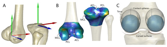
Figure 1.
(A) Anatomical reference frames of the femur and tibia attached to the corresponding bone model were obtained using geometric features of the bone with an automated determination method. (B) The personalized endpoint positions of the knee ligaments were estimated by besting-fitting the statistical shape model (SSM, colored bone model) embedding known endpoint coordinates to the subject’s bone geometry (semitransparent model). The ligament endpoints from the deformed SSM were then projected onto the nearest face of the subject-specific model, determining the personalized ligament endpoint positions. (C) Congruent contact of the tibiofemoral joint was represented by the best-fitted bilateral torus (black dots) and the curved surfaces of tube geometry (red). Contact spheres (blue) nearest to the tibial plateau would also be identified given a specified tibiofemoral 3D pose.
2.2.1. Ligament Endpoints
The generic model of the femur and tibia imbedding ligament endpoints was built based on the statistical shape model (SSM) technique. The SSMs of the femur and tibia were generated using an SSM generation procedure as suggested in [37,38], and a set of CT-derived surface bone models was obtained from 30 healthy male subjects gathered from our former research projects (Ministry of Science and Technology in Taiwan, ROC). Overall, 60 knee joints, consisting of 30 right knees and 30 mirrored left knees, were recruited for building the SSM. The major steps to build an SSM are briefly described below: (i) The CT-derived surface bone models were converted to point distribution models (PDMs) possessing the same number of nodes at corresponding locations using the coherent point drift algorithm [39] (number of nodes: femur = 3051; tibia = 3032); (ii) generalized Procrustes analysis [40] was performed to best align all PDMs under the same reference frame; and (iii) principal component analysis was applied on aligned PDMs to establish an SSM consisting of a mean shape and modes of shape variations. A new shape (a new point cloud) can be thereafter generated by superposing deformations, controlled by parameters of shape variation modes, onto the mean shape.
Bone templates carrying ligament endpoint coordinates are available in the literature [35], which enables reasonably accurate estimation of personalized ligament endpoint locations, free from the requirement of MR imaging. To attach ligament endpoints onto the SSM, the SSMs of the femur and tibia were deformed and rigidly transformed to match the bone templates by minimizing the sum of squared point-to-face distances. The ligament endpoints were projected onto the nearest triangular face of the deformed SSM and expressed in a barycentric coordinate system. Through this procedure, the SSM of the femur and tibia imbedding the corresponding ligament endpoint were obtained. It can thereafter be used to best fit the CT-derived subject-specific bone models of the subject under analysis through the previously mentioned SSM deformation and rigid transformation procedure (Figure 1B). The barycentric coordinates of ligament endpoints from the deformed SSM were converted to Cartesian coordinates and were subsequently projected onto the nearest face of the subject-specific bone model and expressed in the corresponding anatomical reference frame. In this way, the estimated personalized ligament endpoint locations were obtained for each subject (Figure 1B).
2.2.2. Ligament Length
The ligament length was simply defined as the linear distance of respective endpoint positions (Figure 2A), and the length variation during tibiofemoral motion was predicted using a random forest (RF) model. In the current study, the ratio, , between the 3D ligament length () and its projected 2D ligament length () on the mid-sagittal plane was assumed to be associated with tibiofemoral motion and was subject-specific. To provide personalized ligament length variation during entire activity, for each ligament, an RF model was trained to predict this ratio at each instant. The input feature vector was composed of the ratio obtained from the non-weight-bearing extended tibiofemoral pose (i.e., during CT scan), , and the deviations of flexion/extension (FE), adduction/abduction (AA), internal/external rotation (IER), anterior/posterior (AP) translation and proximal/distal (PD) translation of tibiofemoral joint with respect to values at fully extended tibiofemoral pose. The subject- and task-specific lengths of the ACL, PCL and MCL at each instant were thereafter predicted following a leave-one-out cross-validation scheme, in which all the kinematic data reconstructed using the validated MBT approach [20] from the other five subjects (excluding the subject under analysis) were used to train the RF model.
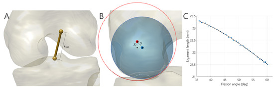
Figure 2.
(A) The ligament length (L3D) was estimated by computing the linear distance between endpoints on the femur and tibia. (B) The shift (S) and vertical shift (SV) of the contact sphere with respect to the centroid axis of the curved surface of the tibial plateau were taken to account for the violation of ideal joint congruency. The blue and red circles represent cross sections of the contact sphere and the tube model, respectively. (C) A 3rd-order polynomial function fitting to the discrete ligament lengths obtained from the registered tibiofemoral kinematics was intended to provide subject- and task-specific representation of ligament elongation along with the knee flexion angles.
Errors of the estimated ligament length were determined by the differences between model-determined and those derived from the tibiofemoral kinematics reconstructed using the biplane MBT. Root-mean-squared (RMS) errors were calculated over all image frames for each subject. The efficacy of the approach was evaluated by comparing the estimated using the model-predicted and constant . The Wilcoxon signed rank test was employed for statistical comparison at a significance level of 0.05.
2.3. Multibody Model-Based Tracking Scheme
The proposed MbMBT scheme mainly consisted of three steps (Figure 3): (i) single-body 3D/2D image registration; (ii) multibody image registration (MIR) with two-level optimization designated to correct the joint dislocation; and (iii) MIR with a hybrid objective function and refined kinematics model.
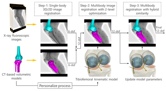
Figure 3.
The overall scheme of the proposed multibody model-based tracking method. A three-step 3D/2D image registration was implemented to successively improve the reproduction of tibiofemoral 3D poses.
2.3.1. Single-Body 3D/2D Image Registration
The first estimation of pose parameters of each bone model (expressed via rigid transformation, ) was determined through an existing single-body 3D/2D image registration approach [21]. To reproduce the projection geometry of the fluoroscopy system, a perspective projection model featuring the focal point, focal length and virtual image plane was reconstructed using a custom-made calibration object [21]. A global reference frame () was defined originating at the bottom left corner of the image plane with the x- and y-axes directed parallel to the image plane and the z-axis normal to the plane. Within the field of view of the projection model, transformation of the volumetric bone model with respect to was estimated by best fitting its DRR to the fluoroscopic image. Normalized cross-correlation of image gradient (GC) was used to quantify the similarity between the DRRs and fluoroscopic images [29]. A genetic algorithm (GA; population size = 50; no. of generations = 60) was employed as the optimizer to search for optimal transformation (design variables: 6 degrees of freedom (6-DOF) of the bone) such that the GC values were maximized.
For each image frame, given the registered transformation, deviations of FE, AA, IER and AP and PD translations of the tibiofemoral joint with respect to those at the extended tibiofemoral pose were calculated. These kinematic deviations together with were fed into the trained RF model to predict for each ligament. At the same time, the registered transformations were used to compute . Multiplication of and would yield an estimation of used for the subsequent multibody image registration.
2.3.2. Multibody Image Registration with Two-Level Optimization
In the second step of the MbMBT, a two-level optimization scheme [21] with MIR was employed to correct artifactual tibiofemoral dislocation. To this end, the femur and tibia/fibula models were simultaneously registered to the fluoroscopic image (Figure 4A) while minimizing the deformations of the personalized tibiofemoral kinematic model. In the outer-level optimization, an overall 11 parameters describing 6-DOF of the femur and 5-DOF of the tibia/fibula (excluding z-axis translation) were taken as the design variables, whereas the remaining parameter was the design variable in the inner-level optimization. In the scheme of the two-level optimization, given each set of outer-level 11-parameters, an inner-level subproblem is solved that gives an optimal solution for tibial z-axis translation. The outer- and optimally inner-level parameters were then joined together to spatially transform the volumetric models of the femur and tibia/fibula, from which the combined DRR was generated (Figure 4B). The outer-level optimization thereafter took the GC values between the combined DRRs and the fluoroscopic image as the objective function value.
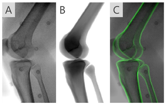
Figure 4.
(A) X-ray fluoroscopic image of the knee joint during a tested activity and (B) the combined digitally reconstructed radiograph (DRR) of both the femur and tibia given the registered pose parameters. (C) The DRR overlaid on the fluoroscopic images visually showed the agreement between the two images.
In the inner-level subproblem, the outer-level 11-parameters served as the fixed parameters, the tibial z-axis translation () was determined as the resultant tibiofemoral pose led to minimize ligament elongation relative to and the shift of contact spheres of the bilateral condyles () with respect to the tube central axis in the corresponding tibial plateau (Figure 2B). To this end, Brent’s algorithm [41] was employed to solve the following equation:
where indicates the ligament length obtained by the resultant tibiofemoral pose, and represent different ligaments and joint compartments, respectively.
After completion of image registration over entire images, the registered transformations of the femur and tibia/fibula were used to derive the length of the ligament at each instant. Meanwhile, the magnitudes of PD compression of the joint, as characterized by the vertical shift of the contact spheres with respect to the tube central axis, , were obtained (Figure 2B). A third-order polynomial equation was fitted to each of the abovementioned parameters against the flexion angles (), given parametric models of ligament length, , and the models of joint compression, (Figure 2C). These parametric models were intended to provide a simplified description of subject-specific, motion-related and smoothly continuous soft tissue deformations of the tibiofemoral joint.
2.3.3. Multibody Image Registration with Hybrid Similarity Measure
The third step of MbMBT aimed to find compromises and , such that the combined DRR best matched the fluoroscopic image (Figure 4C) while complying with the geometric constraints provided by the joint kinematic model. To achieve this goal, a hybrid objective function consisted of an image similarity term defined as the GC values between the DRR () and the fluoroscopic image () and a kinematic model term. The 12-DOF of the femur and tibia are design variables of the optimization. The objective function was formulated as follows,
where denotes the number of elements, is an empirical parameter controlling the weight of the kinematic model term and indicates the PD compressions in bilateral joint compartments obtained by the resultant tibiofemoral pose.
2.4. Evaluation of MbMBT
For each subject, the subject-specific volumetric model of the femur and tibia/fibula were registered to ML view fluoroscopic images in each motion trial using the proposed MbMBT procedure, giving MbMBT-determined bone pose parameters. The standard reference poses of the bone were also determined with corresponding biplane images using a validated biplane MBT method [20]. Given the measured bone pose parameters, tibiofemoral kinematics were calculated following the convention proposed by Grood and Suntay [42]. The degree of agreement between MbMBT-determined kinematics and reference kinematics was evaluated via a coefficient of determination (R2). Differences between MbMBT-determined and reference kinematic variables were computed. For each motion trial, mean absolute differences (MAD), mean differences (denoted as bias) and standard deviation (SD) of differences (denoted as precision) over all image frames were quantified. The means and SDs of the MAD, bias and precision across all subjects were computed. The Wilcoxon signed-rank test was applied to perform between-method comparisons of kinematic variables. The statistical analyses were conducted using MATLAB.
3. Results
The lengths of the ACL, PCL, and MCL predicted with the random forest regression model were compared with standard reference values derived using the biplane MBT-determined tibiofemoral kinematics and the predicted values using a uniform scaling factor (Figure 5A–C) and were shown to have average RMS errors of 0.55 mm, 0.21 mm and 0.14 mm, respectively (Figure 5D). The model-predicted PCL length was significantly more accurate than that obtained using a uniform scaling factor (Figure 5D). While the model-predicted MCL length was not significantly more accurate, the averaged RMS error was nearly half the values obtained using a uniform scaling factor (0.14 mm vs. 0.26 mm, Figure 5D).
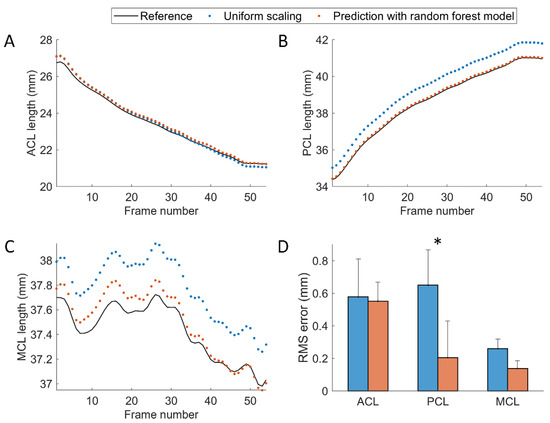
Figure 5.
The length variation of the (A) ACL, (B) PCL, and (C) MCL obtained using the biplane MBT-determined bone poses (black solid lines) and predicted via uniform scaling factor (blue dots) and the random forest model (orange dots). The data were obtained from a typical subject performing lunge activity. (D) The root-mean-squared (RMS) errors of the predicted ligament lengths obtained using uniform scaling factors and the random forest models. The asterisk indicates the significant differences in RMS error between the two methods.
The MADs of 6-DOF of individual bone obtained using single-body model-based tracking (SbMBT, equivalent to step-1 of MbMBT) and the proposed MbMBT are shown in Figure 6, in which the median values of MAD for in-plane translations (X-axis, Y-axis) and rotation (Z-axis) were all below 0.3 mm and 0.2°, respectively. However, the median MADs of the SbMBT- and MbMBT-determined out-of-plane translations (Z-axis) were 3.5 mm and 3.0 mm, respectively. The median values of MAD in out-of-plane rotation components were in the range of 0.3° to 0.8° for the two methods. No significant differences were found in any motion component.
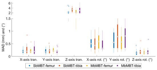
Figure 6.
Boxplot of the mean absolute differences (MADs) of six pose parameters of the femur and tibia-fibula determined using single-body model-based tracking (SbMBT) and multibody model-based tracking (MbMBT). The central marks indicate the median values. The top and bottom sides of the solid box represent the 75th and 25th percentiles of the MAD distribution, respectively. The whiskers indicate the extreme values, and the outliers are drawn with hollow circles.
For the description of tibiofemoral kinematics during isolated knee flexion, MbMBT-determined joint center translations were shown to have precision values less than 1.1 mm and significantly more precise than those obtained with SbMBT (Table 1). A similar tendency can also be found in the MAD metrics (Table 1). No considerable differences were found in rotation components between the two methods, except for Add/Abd bias, for which the MbMBT yielded a slightly lower bias (0.5 ± 1.2°) (Table 1). The MbMBT enabled the reproduction of Flex/Ext, I/E rotation and A/P translation highly representative of standard reference kinematics (R2 > 0.95), moderately representative of joint translation in P/D and L/M components (R2: 0.59–0.70) and weakly representative of Add/Abd (Table 1).

Table 1.
The means ± standard deviations of the mean absolute differences (MAD), bias and precision values over all subjects for six degree-of-freedom kinematics of the knee joint during isolated flexion. The coefficient of determination values (R2) were obtained from linear regression analysis on the knee kinematics derived from the SbMBT and MbMBT methods against reference values. Asterisks indicate significant differences in the variables between the MbMBT and SbMBT.
For the measurement of lunge activity, precision values were less than 0.6 mm in MbMBT-determined translations and 0.4° in rotations, in which three translation components and Add/Abd were significantly more precise in the MbMBT method (Table 2).
Table 2.
The means ± standard deviations of the mean absolute differences (MAD), bias and precision values over all subjects for six degree-of-freedom kinematics of the knee joint during lunge activity. The coefficient of determination values (R2) were obtained from linear regression analysis on the knee kinematics derived from the SbMBT and MbMBT methods against the reference values. Asterisks indicate significant differences in the variables between the MbMBT and SbMBT.
During the sit-to-stand motor task, the MbMBT gave precision values less than 1.0 mm in translations and 1.0° in rotations (Table 3). The use of MbMBT yielded significantly more precise 6-DOF kinematics of the tibiofemoral joint than the SbMBT method (Table 3). The MADs in the rotation components were also significantly smaller with the proposed MbMBT method (Table 3).
Table 3.
The means ± standard deviations of the mean absolute differences (MAD), bias, and precision values over all subjects for six degree-of-freedom kinematics of the knee joint during sit-to-stand. The coefficient of determination values (R2) were obtained from linear regression analysis on the knee kinematics derived from the SbMBT and MbMBT methods against the reference values. Asterisks indicate significant differences in the variables between the MbMBT and SbMBT.
The degree of agreement between the MbMBT-determined kinematics and the reference values during the two weight-bearing activities were greater than 0.94 and 0.92, respectively, except for the LM translation (Table 2 and Table 3). While the LM translation was still the least accurate component, improvements in MAD, precision and degree of agreement over the SbMBT were observed (Table 2 and Table 3).
4. Discussion
A new MbMBT scheme considering the kinematic constraints provided by the personalized model of the tibiofemoral joint was developed in the current study. In general, the MbMBT approach could more precisely determine the 3D tibiofemoral kinematics than the conventional SbMBT, especially in the translation components (Table 1, Table 2 and Table 3). This improvement can be attributed to the proposed tibiofemoral joint models, as they provide physical constraints to prevent the nonphysiological motion of the tibia relative to the femur. Simultaneous image registration of the two bones also helps ensure that the originally accurate kinematic components from the SbMBT would not be compromised by joint model imperfection and motion-related kinematic variability. However, the personalized kinematic model was shown to not effectively diminish the 6-DOF errors of individual bones (Figure 6), similar to the strategies of the anti-collision maneuver at the joint [30,31].
To better reflect the physiological deformation of the ligament in the joint model, the present study first estimated the ligament length in 3D space (i.e., ) from its sagittal plane projection length (i.e., ) using the trained RF model with the prior tibiofemoral kinematics obtained from single-body 3D/2D image registration (step-1). The approach was developed to account for the fact that the ligament length changes along with the tibiofemoral motion [43] and presents individual differences. Since the fluoroscopic detector is often configured to capture ML view images of the knee joint, the out-of-plane translation error of the bone should have a minor influence on the estimation of the . Thus, the relatively accurate was taken to serve as the baseline length of the ligament, and its scaling factors to were predicted with the trained model. The results indicated that the predicted scaling could yield significantly more accurate PCL lengths than those obtained with uniform scaling (Figure 5D). The length of the ACL predicted with RF regression showed the least accurate result among the three ligaments, in which the RMS error was near 0.6 mm close to that obtained with uniform scaling (Figure 5D). This may indicate that the scaling factors between the sagittal and 3D lengths of the ACL were not sufficiently explained by tibiofemoral motions. Further exploration is required to better predict the ACL length variation.
The presented three-step MbMBT scheme originated from the observations that the SbMBT using single-plane images could normally determine accurate in-plane translations and rotations, moderate accuracies in out-of-plane rotations and poor out-of-plane translations [21,25,28], which often propagated to result in artifactual tibiofemoral dislocation. Thus, the MIR with two-level optimization in step-two was designed to solely amend the z-axis translation of the tibia by the tibiofemoral kinematic model, while the other DOFs were merely fine-tuned to ensure image matching between the DRR and the fluoroscopic image. With the strategy, the outer-level optimization left the control of the least accurate z-axis translation to the inner-level subproblem, where the tibiofemoral model dominates the relative z-axis translation of two bones. After completion of the step-two analysis, the model parameters, including variations in ligament length and joint compression, were updated according to the tibiofemoral kinematics to better represent the “subject-specific” and “motion-related” soft tissue deformation during a particular task. Polynomial fitting can also ensure the smoothness of the tissue deformation against knee flexion, which enables improvement of the smoothness of tibiofemoral motion across multiple image frames under the guidance of the joint model in step-three analysis.
The kinematic constraints provided by the personalized tibiofemoral model were demonstrated to effectively ameliorate three-axis translational precision of the joint during all the tested functional activities (Table 1, Table 2 and Table 3). In particular, the L/M translation, typically the least accurate component in SbMBT, obtained an over 65% improvement in precision (average precision values: from 3.6 mm to 1.1 mm during isolated flexion, from 3.2 mm to 0.6 mm during lunge, and from 2.9 mm to 1.0 mm during sit-to-stand; Table 1, Table 2 and Table 3). This improvement might be attributed to the step-two analysis, where the two-level optimization effectively separates the guidance of the joint model on the out-of-plane translation (z-axis) of the tibia. The other 11-DOFs were thereafter fine-tuned given the model-determined tibial z-axis translation to maximize the image registration criteria. This compromise strategy between the kinematic model and the image matching was shown to not notably influence the accuracies in individual bone 6-DOFs (Figure 6) but slightly adjusted the relative poses of the two bones to increase the precision in determining the three translation components (Table 1, Table 2 and Table 3).
In the present study, the contribution of the personalized kinematic model to the accuracy of tibiofemoral rotations was relatively minor (Table 1, Table 2 and Table 3). The reasons may be twofold. First, the SbMBT-determined Flex/Ext and I/E rotation during the three activities were sufficiently representative of standard reference kinematics, as revealed in agreement analysis where the R2 values were above 0.98. The capability of the model is not adequate to further diminish the errors in these two components owing to the model imperfections and uncertainties in the model parameters. Second, our MbMBT strategy was not intended to strictly guide the joint rotations by the kinematic model, as the most suitable model parameters for a particular motion task were unknown. In other words, discrepant tibiofemoral rotation patterns are sure to result in different behaviors in ligament elongation [43,44] and articular contacts [45] and should have different settings for the model parameters. Therefore, such subject-specific and motion-related model parameters were represented by polynomial equations determined using tibiofemoral kinematics after the completion of step-two analysis. The role of the kinematic model in the determination of joint rotations was to provide physical constraints to the bone pose during image registration, which enabled eliminating largely deviated joint angles and improving the angle smoothness throughout the motion task. The effectiveness of the model could be observed in the Add/Abd component (Table 1, Table 2 and Table 3), in which the R2 values were slightly increased with the MbMBT approach. The precision values were also statistically improved in the two weight-bearing tasks (Table 2 and Table 3).
The model inaccuracy is believed to have an impact on the performance of the MbMBT. In the current study, subject-specific ligament insertion points were not available, as MR images were absent. Instead, bone templates embedding known ligament endpoints were deformed to predict the subject’s ligament insertion sites. However, the subjects enrolled in the present study were young Chinese people, but the reference ligament endpoint coordinates were not obtained from similar groups [35]. Potential morphological differences may be present in the bones and soft tissues among different ethnic groups and ages. Some studies have shown morphological differences in the knee [46] and ankle [47] joints between Caucasian and Chinese populations. A validation study is also required to assess the endpoint prediction accuracy and its influences on the performance of the MbMBT in the determination of tibiofemoral kinematics.
5. Conclusions
The present study proposed a new framework to integrate single-plane fluoroscopy and a kinematic model of the tibiofemoral joint for the measurement of 3D tibiofemoral kinematics. The new MbMBT scheme considering the kinematic constraints provided by the personalized kinematic model has been evaluated in vivo. The kinematic model, which consisted of three ligaments and an articular contact mechanism, was shown to help amend the nonphysiological motion of the tibia relative to the femur. The MbMBT was demonstrated to provide a more precise determination of the tibiofemoral kinematics in comparison to the SbMBT in all the tested motion tasks. In further studies, if subject-specific parameters regarding the ligament endpoints and elongation patterns are available, the presented kinematic model may be beneficial to further improve the performance of the MbMBT.
Author Contributions
Each author’s contribution to the article is subdivided as follows: Conceptualization, C.-C.L. and T.-W.L.; methodology, C.-C.L. and H.-L.L.; software, C.-C.L. and J.-D.L.; validation, J.-D.L. and M.-Y.K.; formal analysis, C.-C.L. and C.-Y.W.; investigation, C.-C.L., T.-W.L., H.-L.L., C.-Y.W., J.-D.L., M.-Y.K., and H.-C.H.; resources, C.-C.L. and H.-C.H.; data curation, C.-Y.W. and H.-C.H.; writing—original draft preparation, C.-C.L. and H.-L.L.; writing—review and editing, T.-W.L., C.-Y.W., M.-Y.K., and H.-C.H.; visualization, C.-C.L.; supervision, T.-W.L. and M.-Y.K.; project administration, M.-Y.K., T.-W.L. and H.-C.H.; funding acquisition, C.-C.L., T.-W.L. and H.-C.H. All authors have read and agreed to the published version of the manuscript.
Funding
This research was financially supported by the Ministry of Science and Technology, Taiwan, R.O.C. (MOST 109–2221-E-030–002 -MY2).
Institutional Review Board Statement
The study was conducted following the guidelines of the Declaration of Helsinki and approved by the China Medical University and Hospital Research Ethics Committee.
Informed Consent Statement
Informed consent was obtained from all subjects involved in the current study.
Data Availability Statement
The datasets used in the current study are available from the corresponding author on reasonable request.
Acknowledgments
The authors gratefully acknowledge the staff of the China Medical University Hospital for their assistance in image data collection.
Conflicts of Interest
The authors declare no conflict of interest. The funders had no role in the design of the study; in the collection, analyses, or interpretation of data; in the writing of the manuscript; or in the decision to publish the results.
References
- Hume, D.R.; Kefala, V.; Harris, M.D.; Shelburne, K.B. Comparison of Marker-Based and Stereo Radiography Knee Kinematics in Activities of Daily Living. Ann. Biomed. Eng. 2018, 46, 1806–1815. [Google Scholar] [CrossRef] [PubMed]
- Li, J.-D.; Lu, T.-W.; Lin, C.-C.; Kuo, M.-Y.; Hsu, H.-C.; Shen, W.-C. Soft tissue artefacts of skin markers on the lower limb during cycling: Effects of joint angles and pedal resistance. J. Biomech. 2017, 62, 27–38. [Google Scholar] [CrossRef] [PubMed]
- Veldpaus, F.E.; Woltring, H.J.; Dortmans, L.J.M.G. A least-squares algorithm for the equiform transformation from spatial marker co-ordinates. J. Biomech. 1988, 21, 45–54. [Google Scholar] [CrossRef]
- Lu, T.W.; O’Connor, J.J. Bone position estimation from skin marker co-ordinates using global optimisation with joint constraints. J. Biomech. 1999, 32, 129–134. [Google Scholar] [CrossRef]
- Leardini, A.; Belvedere, C.; Nardini, F.; Sancisi, N.; Conconi, M.; Parenti-Castelli, V. Kinematic models of lower limb joints for musculo-skeletal modelling and optimization in gait analysis. J. Biomech. 2017, 62, 77–86. [Google Scholar] [CrossRef] [PubMed]
- Richard, V.; Cappozzo, A.; Dumas, R. Comparative assessment of knee joint models used in multi-body kinematics optimisation for soft tissue artefact compensation. J. Biomech. 2017, 62, 95–101. [Google Scholar] [CrossRef][Green Version]
- Ojeda, J.; Martínez-Reina, J.; Mayo, J. A method to evaluate human skeletal models using marker residuals and global optimization. Mech. Mach. Theory 2014, 73, 259–272. [Google Scholar] [CrossRef]
- Reinbolt, J.A.; Schutte, J.F.; Fregly, B.J.; Koh, B.I.; Haftka, R.T.; George, A.D.; Mitchell, K.H. Determination of patient-specific multi-joint kinematic models through two-level optimization. J. Biomech. 2005, 38, 621–626. [Google Scholar] [CrossRef]
- Andersen, M.S.; Benoit, D.L.; Damsgaard, M.; Ramsey, D.K.; Rasmussen, J. Do kinematic models reduce the effects of soft tissue artefacts in skin marker-based motion analysis? An in vivo study of knee kinematics. J. Biomech. 2010, 43, 268–273. [Google Scholar] [CrossRef]
- Richard, V.; Lamberto, G.; Lu, T.-W.; Cappozzo, A.; Dumas, R. Knee Kinematics Estimation Using Multi-Body Optimisation Embedding a Knee Joint Stiffness Matrix: A Feasibility Study. PLoS ONE 2016, 11, e0157010. [Google Scholar] [CrossRef]
- Gasparutto, X.; Sancisi, N.; Jacquelin, E.; Parenti-Castelli, V.; Dumas, R. Validation of a multi-body optimization with knee kinematic models including ligament constraints. J. Biomech. 2015, 48, 1141–1146. [Google Scholar] [CrossRef]
- Clément, J.; Dumas, R.; Hagemeister, N.; de Guise, J.A. Soft tissue artifact compensation in knee kinematics by multi-body optimization: Performance of subject-specific knee joint models. J. Biomech. 2015, 48, 3796–3802. [Google Scholar] [CrossRef] [PubMed]
- Duprey, S.; Cheze, L.; Dumas, R. Influence of joint constraints on lower limb kinematics estimation from skin markers using global optimization. J. Biomech. 2010, 43, 2858–2862. [Google Scholar] [CrossRef]
- Feikes, J.D.; O’Connor, J.J.; Zavatsky, A.B. A constraint-based approach to modelling the mobility of the human knee joint. J. Biomech. 2003, 36, 125–129. [Google Scholar] [CrossRef]
- Sancisi, N.; Parenti-Castelli, V. A New Kinematic Model of the Passive Motion of the Knee Inclusive of the Patella. J. Mech. Robot. 2011, 3, 041003. [Google Scholar] [CrossRef]
- Brito da Luz, S.; Modenese, L.; Sancisi, N.; Mills, P.M.; Kennedy, B.; Beck, B.R.; Lloyd, D.G. Feasibility of using MRIs to create subject-specific parallel-mechanism joint models. J. Biomech. 2017, 53, 45–55. [Google Scholar] [CrossRef] [PubMed]
- Nardini, F.; Belvedere, C.; Sancisi, N.; Conconi, M.; Leardini, A.; Durante, S.; Parenti-Castelli, V. An Anatomical-Based Subject-Specific Model of In-Vivo Knee Joint 3D Kinematics from Medical Imaging. Appl. Sci. 2020, 10, 2100. [Google Scholar] [CrossRef]
- Flood, P.D.L.; Banks, S.A. Automated Registration of 3-D Knee Implant Models to Fluoroscopic Images Using Lipschitzian Optimization. IEEE Trans. Med. Imaging 2018, 37, 326–335. [Google Scholar] [CrossRef]
- Markelj, P.; Tomaževič, D.; Likar, B.; Pernuš, F. A review of 3D/2D registration methods for image-guided interventions. Med. Image Anal. 2012, 16, 642–661. [Google Scholar] [CrossRef]
- Lin, C.-C.; Lu, T.-W.; Li, J.-D.; Kuo, M.-Y.; Kuo, C.-C.; Hsu, H.-C. An automated three-dimensional bone pose tracking method using clinical interleaved biplane fluoroscopy systems: Application to the knee. Appl. Sci. 2020, 10, 8426. [Google Scholar] [CrossRef]
- Lin, C.-C.; Li, J.-D.; Lu, T.-W.; Kuo, M.-Y.; Kuo, C.-C.; Hsu, H.-C. A model-based tracking method for measuring 3D dynamic joint motion using an alternating biplane x-ray imaging system. Med. Phys. 2018, 45, 3637–3649. [Google Scholar] [CrossRef] [PubMed]
- Barré, A.; Aminian, K. Error performances of a model-based biplane fluoroscopic system for tracking knee prosthesis during treadmill gait task. Med. Biol. Eng. Comput. 2018, 56, 307–316. [Google Scholar] [CrossRef]
- Guan, S.; Gray, H.A.; Keynejad, F.; Pandy, M.G. Mobile Biplane X-Ray Imaging System for Measuring 3D Dynamic Joint Motion During Overground Gait. IEEE Trans. Med. Imaging 2016, 35, 326–336. [Google Scholar] [CrossRef]
- Ivester, J.C.; Cyr, A.J.; Harris, M.D.; Kulis, M.J.; Rullkoetter, P.J.; Shelburne, K.B. A Reconfigurable High-Speed Stereo-Radiography System for Sub-Millimeter Measurement of In Vivo Joint Kinematics. J. Med. Devices 2015, 9, 041009. [Google Scholar] [CrossRef]
- Postolka, B.; List, R.; Thelen, B.; Schütz, P.; Taylor, W.R.; Zheng, G. Evaluation of an intensity-based algorithm for 2D/3D registration of natural knee videofluoroscopy data. Med. Eng. Phys. 2020, 77, 107–113. [Google Scholar] [CrossRef] [PubMed]
- Lawrence, R.L.; Ellingson, A.M.; Ludewig, P.M. Validation of single-plane fluoroscopy and 2D/3D shape-matching for quantifying shoulder complex kinematics. Med. Eng. Phys. 2018, 52, 69–75. [Google Scholar] [CrossRef]
- Ellingson, A.M.; Mozingo, J.D.; Magnuson, D.J.; Pagnano, M.W.; Zhao, K.D. Characterizing fluoroscopy based kinematic accuracy as a function of pulse width and velocity. J. Biomech. 2016, 49, 3741–3745. [Google Scholar] [CrossRef]
- Tsai, T.Y.; Lu, T.W.; Chen, C.M.; Kuo, M.Y.; Hsu, H.C. A volumetric model-based 2D to 3D registration method for measuring kinematics of natural knees with single-plane fluoroscopy. Med. Phys. 2010, 37, 1273–1284. [Google Scholar] [CrossRef]
- Penney, G.P.; Weese, J.; Little, J.A.; Desmedt, P.; Hill, D.L.G.; Hawkes, D.J. A comparison of similarity measures for use in 2-D-3-D medical image registration. IEEE Trans. Med. Imaging 1998, 17, 586–595. [Google Scholar] [CrossRef]
- Prins, A.H.; Kaptein, B.L.; Stoel, B.C.; Reiber, J.H.C.; Valstar, E.R. Detecting femur–insert collisions to improve precision of fluoroscopic knee arthroplasty analysis. J. Biomech. 2010, 43, 694–700. [Google Scholar] [CrossRef]
- Lin, C.-C.; Lu, T.-W.; Shih, T.-F.; Tsai, T.-Y.; Wang, T.-M.; Hsu, S.-J. Intervertebral anticollision constraints improve out-of-plane translation accuracy of a single-plane fluoroscopy-to-CT registration method for measuring spinal motion. Med. Phys. 2013, 40, 031912. [Google Scholar] [CrossRef]
- El Habachi, A.; Moissenet, F.; Duprey, S.; Cheze, L.; Dumas, R. Global sensitivity analysis of the joint kinematics during gait to the parameters of a lower limb multi-body model. Med. Biol. Eng. Comput. 2015, 53, 655–667. [Google Scholar] [CrossRef]
- Rachmat, H.H.; Janssen, D.; Zevenbergen, W.J.; Verkerke, G.J.; Diercks, R.L.; Verdonschot, N. Generating finite element models of the knee: How accurately can we determine ligament attachment sites from MRI scans? Med. Eng. Phys. 2014, 36, 701–707. [Google Scholar] [CrossRef]
- Bergamini, E.; Pillet, H.; Hausselle, J.; Thoreux, P.; Guerard, S.; Camomilla, V.; Cappozzo, A.; Skalli, W. Tibio-femoral joint constraints for bone pose estimation during movement using multi-body optimization. Gait Posture 2011, 33, 706–711. [Google Scholar] [CrossRef] [PubMed][Green Version]
- Pillet, H.; Bergamini, E.; Rochcongar, G.; Camomilla, V.; Thoreux, P.; Rouch, P.; Cappozzo, A.; Skalli, W. Femur, tibia and fibula bone templates to estimate subject-specific knee ligament attachment site locations. J. Biomech. 2016, 49, 3523–3528. [Google Scholar] [CrossRef] [PubMed]
- Miranda, D.L.; Rainbow, M.J.; Leventhal, E.L.; Crisco, J.J.; Fleming, B.C. Automatic determination of anatomical coordinate systems for three-dimensional bone models of the isolated human knee. J. Biomech. 2010, 43, 1623–1626. [Google Scholar] [CrossRef] [PubMed]
- Tsai, T.-Y.; Li, J.-S.; Wang, S.; Li, P.; Kwon, Y.-M.; Li, G. Principal component analysis in construction of 3D human knee joint models using a statistical shape model method. Comput. Methods Biomech. Biomed. Eng. 2015, 18, 721–729. [Google Scholar] [CrossRef] [PubMed]
- Baka, N.; Kaptein, B.L.; de Bruijne, M.; van Walsum, T.; Giphart, J.E.; Niessen, W.J.; Lelieveldt, B.P.F. 2D-3D shape reconstruction of the distal femur from stereo X-ray imaging using statistical shape models. Med. Image Anal. 2011, 15, 840–850. [Google Scholar] [CrossRef]
- Myronenko, A.; Song, X. Point Set Registration: Coherent Point Drift. IEEE Trans. Pattern Anal. Mach. Intell. 2010, 32, 2262–2275. [Google Scholar] [CrossRef]
- Gower, J.C. Generalized procrustes analysis. Psychometrika 1975, 40, 33–51. [Google Scholar] [CrossRef]
- Brent, R.P. Algorithms for Minimization without Derivatives; Courier Corporation: Chelmsford, MA, USA, 2013. [Google Scholar]
- Grood, E.S.; Suntay, W.J. A joint coordinate system for the clinical description of three-dimensional motions: Application to the knee. J. Biomech. Eng. 1983, 105, 136–144. [Google Scholar] [CrossRef] [PubMed]
- Hosseini Nasab, S.H.; List, R.; Oberhofer, K.; Fucentese, S.F.; Snedeker, J.G.; Taylor, W.R. Loading patterns of the posterior cruciate ligament in the healthy knee: A systematic review. PLoS ONE 2016, 11, e0167106. [Google Scholar] [CrossRef] [PubMed]
- Kernkamp, W.A.; Varady, N.H.; Li, J.-S.; Tsai, T.-Y.; Asnis, P.D.; van Arkel, E.R.; Nelissen, R.G.; Gill, T.J.; Van de Velde, S.K.; Li, G. An in vivo prediction of anisometry and strain in anterior cruciate ligament reconstruction–A combined magnetic resonance and dual fluoroscopic imaging analysis. Arthrosc. J. Arthrosc. Relat. Surg. 2018, 34, 1094–1103. [Google Scholar] [CrossRef] [PubMed]
- Johal, P.; Williams, A.; Wragg, P.; Hunt, D.; Gedroyc, W. Tibio-femoral movement in the living knee. A study of weight bearing and non-weight bearing knee kinematics using ‘interventional’MRI. J. Biomech. 2005, 38, 269–276. [Google Scholar] [PubMed]
- Ho, W.-P.; Cheng, C.-K.; Liau, J.-J. Morphometrical measurements of resected surface of femurs in Chinese knees: Correlation to the sizing of current femoral implants. Knee 2006, 13, 12–14. [Google Scholar] [CrossRef]
- Kuo, C.C.; Lu, H.L.; Leardini, A.; Lu, T.W.; Kuo, M.Y.; Hsu, H.C. Three-dimensional computer graphics-based ankle morphometry with computerized tomography for total ankle replacement design and positioning. Clin. Anat. 2014, 27, 659–668. [Google Scholar] [CrossRef]
Publisher’s Note: MDPI stays neutral with regard to jurisdictional claims in published maps and institutional affiliations. |
© 2021 by the authors. Licensee MDPI, Basel, Switzerland. This article is an open access article distributed under the terms and conditions of the Creative Commons Attribution (CC BY) license (https://creativecommons.org/licenses/by/4.0/).