A Semi-Supervised Fault Diagnosis Method Based on Improved Bidirectional Generative Adversarial Network

Abstract

With the assumption of sufficient labeled data, deep learning based machinery fault diagnosis methods show effectiveness. However, in real-industrial scenarios, it is costly to label the data, and unlabeled data is underutilized. Therefore, this paper proposes a semi-supervised fault diagnosis method called Bidirectional Wasserstein Generative Adversarial Network with Gradient Penalty (BiWGAN-GP). First, by unsupervised pre-training, the proposed method takes full advantage of a large amount of unlabeled data and can extract features from vibration signals effectively. Then, using only a few labeled data to conduct supervised fine-tuning, the model can perform an accurate fault diagnosis. Additionally, Wasserstein distance is used to improve the stability of the model’s training procedure. Validation is performed on the bearing and gearbox fault datasets with limited labeled data. The results show that the proposed method can achieve 99.42% and 91.97% of diagnosis accuracy on the bearing and gear dataset, respectively, when the size of the training set is only 10% of the testing set.

1. Introduction

As the essential part of prognostics and health management (PHM), fault diagnosis technology can enhance machinery reliability, increase operating safety, and reduce maintenance costs [1]. For example, the failure of wind turbine bearings, which are mounted at high altitudes and work in harsh conditions, will lead to higher repair costs [2]. Therefore, it is meaningful to develop reliable and accurate fault diagnosis methods for the essential machinery components of machines such as bearings and gears.

With the development of industrial information technology, data-driven methods have become mainstream of intelligent fault diagnosis. As the key process of data-driven methods, the feature extraction ability greatly affects the accuracy of diagnosis [3]. Recently, deep learning based methods have attracted attention—because its ability to automatically extract features, which are less dependent on prior knowledge about signal processing techniques and diagnostic expertise [4]. As the model deepens, the capabilities of feature extraction and abstraction are also enhanced. However, deeper models require more data for training, or the model’s performance may be affected by over-fitting. Therefore, deep learning methods have higher requirements for both quality and quantity of data.

Table 1. Summary of the recent fault diagnosis methods based on deep learning.

	Reference	Method	Objects
Supervised	[5]	One-dimensional convolutional neural network(1-DCNN)	planetary gearbox
	[6]	Deep convolution neural network (DCNN) with wavelet image	rolling bearing
	[7]	Multiple wavelet regularized deep residual network (MWR-DRN)	planetary gearbox
	[8]	Recurrent neural network (RNN) based on gated recurrent units (GRUs)	bearing and pump
Unsupervised	[9]	Local connection network (LCN) constructed by normalized sparse autoencoder (NSAE)	gearbox and bearing
	[10]	Deep sparse autoencoder (DSAE)	gear pitting fault
	[11]	Convolutional deep belief network (CDBN)	rolling bearing
	[12]	Enhanced deep convolutional generative adversarial network (DCGAN)	gearbox and bearing
	[13]	Wavelet packet transform combined with generative adversarial networks (GAN)	robotic manipulator
	[14]	Categorical adversarial autoencoder (CatAAE)	gearbox and bearing
Semi-supervised	[15]	Consistency regularization based semi-supervised learning	rolling bearing
	[16]	semi-supervised deep sparse autoencoder (SSDSAE) with local and nonlocal information	bearing and industrial rotor
	[17]	Graph-based rebalance semi-supervised learning (GRSSL) with visibility graph feature (VGF)	rolling bearing

shows the summary of the recent fault diagnosis methods based on deep learning, including supervised, unsupervised and semi-supervised learning methods. With the assumption of sufficient data, supervised deep learning based fault diagnosis methods show effectiveness. Wu et al. [5] applied the one-dimensional convolutional neural network (1-DCNN) to learn features directly from the raw vibration signals and achieved nearly 100% diagnostic accuracy of the gearbox fault dataset. Duong et al. [6] used the wavelet transform to get the 2D image of the acoustic emission signals of the bearing, then applied a deep convolution neural network (DCNN) as a classifier and achieved an accuracy of 98.79%. Zhao et al. [7] applied the famous deep learning architecture in image processing—deep residual network (ResNet) on the 2D matrices of wavelet coefficient to improve the accuracy of gearbox fault diagnosis and reached an accuracy of 96.67%. Zhang et al. [8] proposed a gated recurrent unit (GRU) based recurrent neural network (RNN) to make full use of the temporal information from time-series signals, the model shows nearly 100% accuracy and can get 94.86% against the −4dB signal-to-noise ratios noise. Similarly, those studies benefited from the high-quality datasets and sufficient training data.

Although we can obtain "big data" due to the development of data acquisition technologies in real industrial scenarios, most of the available data is unlabeled raw data. On the other hand, labeling data is expensive or time-consuming. Therefore, in the case of insufficient labeled data, it is difficult for the supervised deep learning model to show excellent performance. Researchers have been seeking ways to solve this problem, such as unsupervised learning and semi-supervised learning.

Unsupervised deep learning methods such as autoencoders (AE), deep belief networks (DBN), and generative adversarial networks (GAN) have been studied to apply on fault diagnosis tasks. AE can learn features from unlabeled data by reconstructing them. Jia et al. [9] proposed a sparse autoencoder based local connection network that can mine shift-invariant fault features from vibration signals. Qu et al. [10] integrated dictionary learning in sparse coding to extract features from raw data by using a deep sparse autoencoder. DBN is another classic unsupervised learning method, Liu et al. [11] proposed a bearing fault diagnosis method based on improved convolutional DBN to extract quantitative and qualitative features from vibration signals. Recently, GAN [18] has been successfully applied in many fields because of its ability to generate realistic data. Therefore, researchers have developed some applications of GAN and its variants in the field of fault diagnosis. Data augmentation is the most common use of GAN to solve the insufficient or imbalanced problem of fault data. Wang et al. [12] applied a 1-DCNN based deep convolutional generative adversarial network (DCGAN) to enhance the GAN model, then K-means clustering algorithm and ridge regression are used to improve a CNN model for fault classification. Pu et al. [13] used GAN as an oversampling method to compensate the unbalanced dataset for fault diagnosis of an industrial robotic manipulator. Liu et al. [14] combined categorical GAN and adversarial autoencoder to perform unsupervised clustering of rolling bearings.

To make more effective use of both labeled and unlabeled data, semi-supervised learning methods have attracted the attention of researchers. Yu et al. [15] proposed a semi-supervised approach based on consistency regularization principle that makes the model less sensitive to the extra perturbation imposed on the inputs. Zhao et al. [16] embedded the labeled and unlabeled data into local and nonlocal regularization terms to realize a semi-supervised deep sparse autoencoder. Chen et al. [17] proposed a graph-based rebalance semi-supervised learning method, and they mainly focus on variable conditions and imbalance unlabeled data.

This paper proposes a new semi-supervised learning method focusing on the problem of insufficient labeled data, namely Bidirectional Wasserstein Generative Adversarial Network with Gradient Penalty (BiWGAN-GP). Compare to the existing work of semi-supervised fault diagnosis methods, the proposed method makes full use of the representation learning ability of GAN. It not only can extract effective features from the unlabeled data but also can generate realistic signals for data augmentation, which makes it suitable for fault diagnosis tasks with limited labeled data. The main contributions of this paper can be summarized as follows:

(1)

By adding an encoder on the standard GAN architecture, for the first time, bidirectional GAN is introduced in the machinery fault diagnosis field, which provides a new way for automatic feature extraction from unlabeled data.

(2)

Wasserstein distance with gradient penalty is used in the unsupervised training procedure, which improves the model’s stability and usability. Experimental results show the effectiveness and necessity of this improvement.

(3)

With limited labeled data to fine-tune the model’s parameters, the proposed method can achieve a satisfactory diagnosis accuracy, which can reduce the cost of labeling data.

The rest of this article is organized as follows. Section 2 gives the theoretical background about GAN and bidirectional GAN, then the specific methods for improving the GAN are described. Section 3 present the detailed system framework and the training procedure of the proposed method. Experiments are conducted in Section 4 to verify the effectiveness of the proposed method for data generation and fault diagnosis. Finally, the discussion and conclusions are drawn in Section 5 and Section 6, respectively.

2. Methodologies

2.1. Generative Adversarial Networks

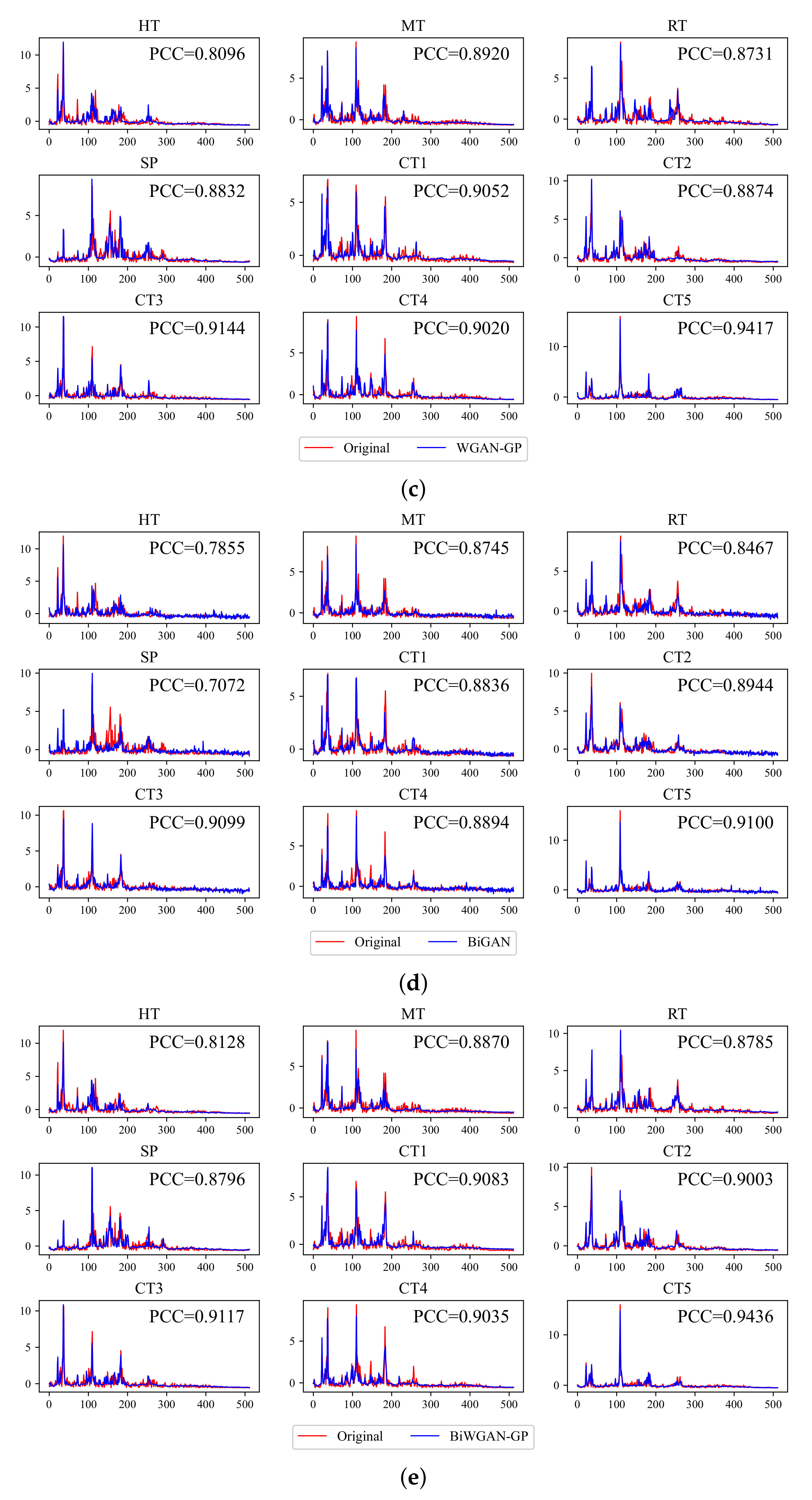
Generative adversarial network (GAN) is a framework that can capture the real data’s distribution and then generate fake data very similar to real data. It consists of two modules: generator G and discriminator D, as shown in Figure 1a.

Different from the traditional generative models, GAN does not compute the exact probability density function $p_X\left(x\right)$ of the data distribution (which is difficult), it models $p_X\left(x\right)$ by transforming a latent distribution $p_Z\left(z\right)$, such as a standard Normal distribution $\mathcal{N}(0,I)$. This transformation is called a generator G, which mapping from the latent feature space to data space by a feed-forward network $\tilde{x}=G\left(z\right),G:{\Omega }_z\to {\Omega }_x$. Another module called discriminator D aims to distinguish between samples from the data space or generator G. Through adversarial training of G and D, $p_G\left(x\right)$ gradually approaches $p_X\left(x\right)$ and finally matches it. Therefore, GAN can learn arbitrarily complex real data distribution and then create real-like data.

The following minimax objective formulates the training of GAN:

$$\begin{array}{cc}\hfill \underset{G}{min}\underset{D}{max}V(D,G)=& {\mathbb{E}}_{x\sim p_X}[logD\left(x\right)]+\hfill \\ \hfill & {\mathbb{E}}_{z\sim p_Z}[log(1-D\left(G\left(z\right)\right))]\hfill \end{array}$$

(1)

where $D\left(x\right)$ represents the probability that discriminator will determine the data x from the true distribution $p_X$ to be true, and $(1-D(G\left(z\right)\left)\right)$ means the probability that D will judge the sample generated by the generator $G\left(z\right)$ is false. The goal of D is to maximize the above probabilities, therefore the loss function of the discriminator is:

$$\begin{array}{cc}\hfill {\mathcal{L}}_D=& -{\mathbb{E}}_{x\sim p_X}[logD\left(x\right)]\hfill \\ \hfill & -{\mathbb{E}}_{z\sim p_Z}[log(1-D\left(G\left(z\right)\right))]\hfill \end{array}$$

(2)

The goal of generator G is to minimize the probability that D successfully discriminates generated samples. The first term of Equation (1) makes no reference to G, so it can be ignored. Therefore the loss function of the generator is:

$${\mathcal{L}}_G={\mathbb{E}}_{z\sim p_Z}[log(1-D\left(G\left(z\right)\right))]$$

(3)

However, in the early training Equation (3) cannot provide enough gradient for the learning of G. In practice, Goodfellow proposed an alternative generator loss function:

$${\mathcal{L}}_G=-{\mathbb{E}}_{z\sim p_Z}[log\left(D\left(G\left(z\right)\right)\right)]$$

(4)

By alternating training G and D, when the algorithm converges, the generated distribution of G coincides with the real data distribution, i.e., $p_G=p_X$, and D will not be able to distinguish whether the sample is real or fake, i.e., $D\left(G\right(z\left)\right)=0.5$.

Compared with the traditional generative model, GAN is simpler to construct and more straightforward to train. However, the original GAN model can only utilize unlabeled data to perform unsupervised learning tasks such as generating fake data. It lacks the ability to perform supervised learning such as classification. For that reason, we have to modify the architecture of GAN for fault diagnosis.

2.2. Bidirectional Generative Adversarial Networks

In order to use GAN’s advantages to capture data distribution for inference and classification tasks, Donahue et al. [19] proposed the bidirectional generative adversarial network (BiGAN) by introducing an additional encoder E on the basis of GAN, which gives BiGAN the ability to extract data features and to perform semi-supervised learning.

As shown in Figure 1b, the obvious difference between BiGAN and GAN is the encoder E. In addition to the generator G that maps the latent space to the data space, BiGAN introduces an encoder E to inversely map the data space to the latent space, i.e., $\tilde{z}=E\left(x\right)$. Thus $\tilde{z}$ can be used as low-dimensional features extracted from data samples by the encoder.

Besides, the structure of discriminator D needs to be modified as well. Instead of taking x or $\tilde{x}=G\left(z\right)$ as the input of D, the discriminator discriminates joint pair $(x,\tilde{z})$ or $(\tilde{x},z)$ from data space and latent space, respectively.

Similarly to GAN, the goal of BiGAN can be defined as a minimax objective:

$$\begin{array}{cc}\hfill \underset{G,E}{min}\underset{D}{max}V(D,E,G)=& {\mathbb{E}}_{x\sim p_X}[logD(x,E(x\left)\right)]+\hfill \\ \hfill & {\mathbb{E}}_{z\sim p_Z}[log(1-D(G\left(z\right),z)]\hfill \end{array}$$

(5)

The goal of D is to maximize the value function $V(D,E,G)$, and the goal of both G and E is to minimize it. In addition, BiGAN also uses the alternative loss function of G as mentioned in Equation (4). So we can obtain the following loss functions for the training of BiGAN:

$$\begin{array}{cc}\hfill {\mathcal{L}}_D=& -{\mathbb{E}}_{x\sim p_X}[logD(x,E(x\left)\right)]\hfill \\ \hfill & -{\mathbb{E}}_{z\sim p_Z}[log(1-D(G\left(z\right),z\left)\right)]\hfill \end{array}$$

(6)

$$\begin{array}{cc}\hfill {\mathcal{L}}_{EG}=& -{\mathbb{E}}_{x\sim p_X}[log(1-D(x,E\left(x\right))]\hfill \\ \hfill & -{\mathbb{E}}_{z\sim p_Z}[logD\left(G\right(z),z)]\hfill \end{array}$$

(7)

The encoder E helps BiGAN extract features from data to perform classification and makes BiGAN suitable for semi-supervised learning tasks.

2.3. Improve the Training of BiGAN

2.3.1. Wasserstein GAN with Gradient Penalty

Although the origin GAN model is simple to construct, a high-quality GAN model is hard to obtain. However, the training of the origin GAN may have problems such as non-convergence and mode collapse. BiGAN has the same problems because it uses similar loss functions [20]. Those issues reduce the usability, that the model not being able to generate samples of all fault types. Therefore, it is necessary to improve the training process of BiGAN.

The inappropriate measurement method causes the difficulty of training [21]. The original GAN optimizes the Jensen–Shannon (JS) divergence between the generated and real distribution. However, when the two distributions do not have any non-negligible intersection, the JS divergence is a constant, which causes the vanishing gradient.

To solve this problem, a new measurement method is proposed, namely Earth Mover distance or Wasserstein distance [22]. Even if the two distributions do not have any overlap, this metric can still indicate the distance between them and provide effective gradients for training. The model built based on Wasserstein distance is called Wasserstein GAN (WGAN). The value function of WGAN is:

$$\underset{G}{min}\underset{D}{max}V(D,G)={\mathbb{E}}_{x\sim p_X}\left[D\left(x\right)\right]-{\mathbb{E}}_{z\sim p_Z}\left[D\left(G\left(z\right)\right)\right]$$

(8)

which is similar to Equation (1) but without taking the logarithm, and alternative G loss is also taken.

Similarly, we can derive the loss function from Equation (8):

$${\mathcal{L}}_D=-{\mathbb{E}}_{x\sim p_X}\left[D\left(x\right)\right]+{\mathbb{E}}_{z\sim p_Z}\left[D\left(G\left(z\right)\right)\right]$$

(9)

$${\mathcal{L}}_G=-{\mathbb{E}}_{z\sim p_Z}\left[D\left(G\left(z\right)\right)\right]$$

(10)

The Equation (9) is also the definition of Wasserstein distance.

In addition to the loss function, the main structural modification of WGAN is about the discriminator D. It removes the sigmoid activation function at the last layer so that the output is no longer limited to (0,1). However, to enforce the Lipschitz constraint, WGAN demands clipping the weight of D with a constant c after every update step, i.e., $w_D\in [-c,c]$. This procedure may cause a phenomenon that the value of $w_D$ always approximates c or $-c$. If c is too large or too small, it may lead to vanishing or exploding gradients.

Therefore, Gulrajani et al. [23] improved WGAN by adding a gradient penalty term in Equation (9), called WGAN-GP. It can avoid weight clipping and enforce the Lipschitz constraint. The loss function of the WGAN-GP’s discriminator is:

$$\begin{array}{cc}\hfill {\mathcal{L}}_D=& -{\mathbb{E}}_{x\sim p_X}\left[D\left(x\right)\right]+{\mathbb{E}}_{z\sim p_Z}\left[D\left(G\left(z\right)\right)\right]\hfill \\ \hfill & +\lambda {\mathbb{E}}_{\widehat{x}\sim p_{\widehat{x}}}\left[\right(\left|\right|{\nabla }_{\widehat{x}}D\left(\widehat{x}\right){\left|\right|}_2-1{)}^2]\hfill \end{array}$$

(11)

where the additional part compared to Equation (9) is the gradient penalty term. $\widehat{x}$ is the linear interpolation between the real data x and the generated data $G\left(z\right)$:

$$\widehat{x}=ϵx+(1-ϵ)G\left(z\right)$$

(12)

where $\lambda$ is penalty coefficient, usually take $\lambda =10$, and $ϵ$ is a random number $ϵ\sim U[0,1]$.

2.3.2. Improve BiGAN with WGAN-GP

Eventually, we use WGAN-GP to improve the training of BiGAN. The model we got is called bidirectional Wasserstein generative adversarial networks with gradient penalty (BiWGAN-GP). The BiWGAN-GP’s discriminator loss function is

$$\begin{array}{cc}\hfill {\mathcal{L}}_D=& -{\mathbb{E}}_{x\sim p_X}[D(x,E\left(x\right)]+{\mathbb{E}}_{z\sim p_Z}\left[D(G\left(z\right),z)\right]\hfill \\ \hfill & +\lambda {\mathbb{E}}_{\widehat{x}\sim p_{\widehat{x}},\widehat{z}\sim p_{\widehat{z}}}\left[\right(\left|\right|{\nabla }_{(\widehat{x},\widehat{z})}D(\widehat{x},\widehat{z}){\left|\right|}_2-1{)}^2]\hfill \end{array}$$

(13)

where $\widehat{x}$ is defined in Equation (12), and $\widehat{z}$ is the linear interpolation between $E\left(x\right)$ and z:

$$\widehat{z}=ϵE\left(z\right)+(1-ϵ)z$$

(14)

The loss function of G and E in BiWGAN-GP can obtain from Equation (8) directly by replacing the input of D with joint pairs:

$$\begin{array}{c}\hfill {\mathcal{L}}_{EG}={\mathbb{E}}_{x\sim p_X}\left[D(x,E\left(x\right))\right]-{\mathbb{E}}_{z\sim p_Z}\left[D(G\left(z\right),z)\right]\end{array}$$

(15)

This equation is also the Wasserstein distance between the real distribution and the generated distribution, which can indicate the training process.

The experiment in Section 4 shows that after using WGAN with gradient penalty to improve BiGAN, the model generation result and the diagnosis accuracy in the case of a small training dataset are improved.

3. System Framework and Model Training

3.1. Model Architecture

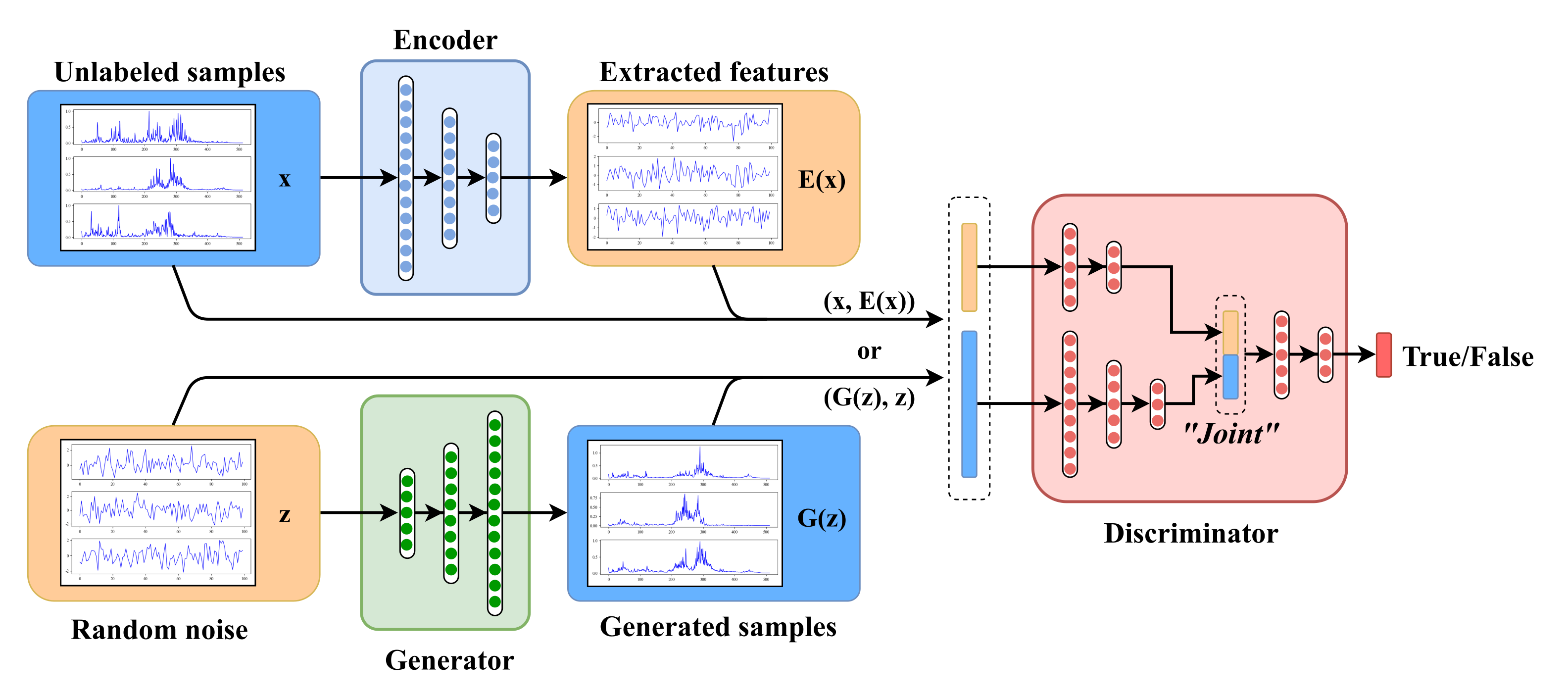
We propose a novel approach to perform both vibration signal generation and machinery fault diagnosis, called BiWGAN-GP. It combined the architecture of BiGAN and the advanced training method of WGAN-GP. Figure 2 Shows the BiWGAN-GP’s architecture. Overall, the BiWGAN-GP fault diagnosis model has three main modules: generator, encoder, and discriminator, respectively.

The generator consists of a multi-layer neural network with an increasing number of hidden units to mapping a low-dimension noise z into a high dimension generated signal $G\left(z\right)$. Therefore, the input dimension of the generator depends on the latent vector z, and the output dimension matches the real signal length. The number of units in the latter hidden layer is double that of the former layer. Specifically, the topology of G is (64, 128, 256, 512).

Different data preprocessing methods will affect the construction of the generator. If normalization is used, i.e., $x^{\prime }=(x-x_{min})/(x_{max}-x_{min})$, the data amplitude is limited to (0,1). Then ReLU activation function is used between the layers of G, and the SoftPlus is used in the last layer to ensure that there is no negative value in generated signals. Another commonly used data preprocessing operation is standardization, i.e., $x^{\prime }=(x-\mu )/\sigma$, where $\mu$ is the mean and $\sigma$ is the standard deviation of the entire dataset. Since standardization may have negative values, to avoid truncation, we use LeakyReLU as the activation function of the last layer of G to get better generation results.

The encoder is also composed of a multi-layer neural network but with a decreasing number of hidden units to extract the most salient features of the data. Specifically, the topology of E is (512, 256, 128, 64), where the number of units in the hidden latter layer is half that of the former layer. Its input and output dimensions are opposite to those of the generator. LeakyReLU is used as the activation function in the encoder.

The discriminator is divided into three parts. Two multi-layer neural networks extract features of the joint pair $(x,E(x\left)\right)$ that comes from real data or $\left(G\right(z),z)$ that comes from fake data, and their topology are (256, 128, 64) and (128, 64). Then the features are concatenated together as a joint feature which size is 128. Finally, through another multi-layer neural network which topology is (128, 64, 32, 1), the discriminatory result is obtained. Also, LeakyReLU is used as the activation function.

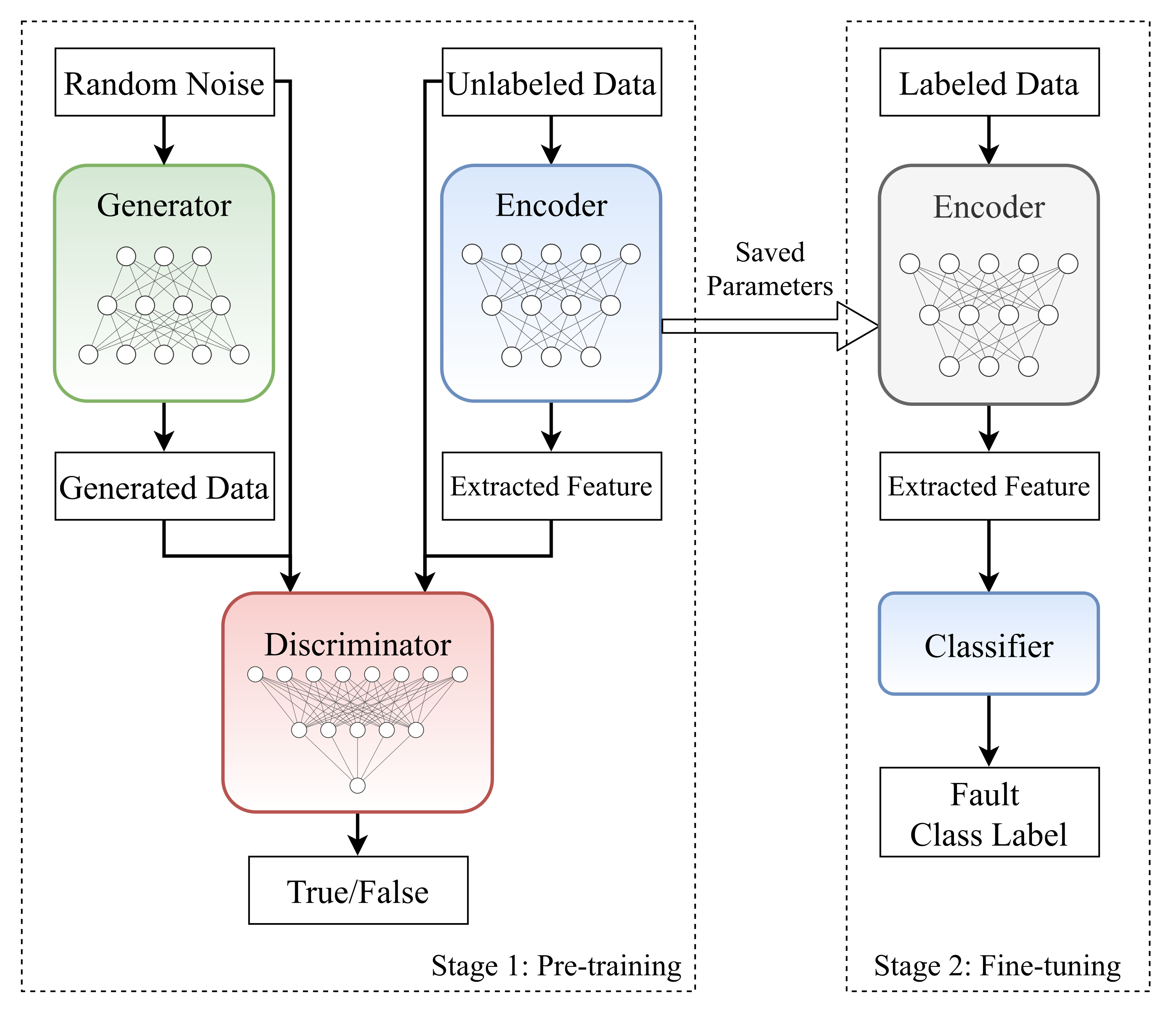
3.2. Model Training Procedure

The training process of the BiWGAN-GP has two stages, namely the unsupervised pre-training stage and the supervised fine-tuning stage. Figure 3 shows the training procedure of the proposed fault diagnosis method.

The unsupervised pre-training procedure is described in Algorithm 1. In this stage, all unlabeled data is used to train the model. Two Adam [24] optimizers are used to update the model parameters, one for the discriminator, corresponding to the loss function (13), and the other one is responsible for optimizing the generator and encoder parameters, corresponding to the loss function (15). Since the Wasserstein distance with gradient penalty is used to improve the loss function, there is no need to worry about the discriminator being trained too well and the convergence problem. After the unsupervised stage, the generator of BiWGAN-GP can be used to generate real-like samples for the data augmentation task.

In the supervised fine-tuning stage, we train the model for fault diagnosis using only a small amount of labeled samples. The encoder network in the BiWGAN-GP model is extracted, and a fully connected layer is appended as a classifier. An Adam optimizer is used to update the parameters of the classifier. Commonly, a typical deep learning model takes more training samples than testing samples. However, to simulate the situation where it is difficult to obtain enough high-quality labeled data for training, this article uses the way that there are far more test samples than training samples in the supervised learning stage.

Algorithm 1: The pre-training procedure of BiWGAN-GP with gradient penalty. Default values: $\lambda =10,\alpha =0.0001,{\beta }_1=0.5,{\beta }_2=0.999$

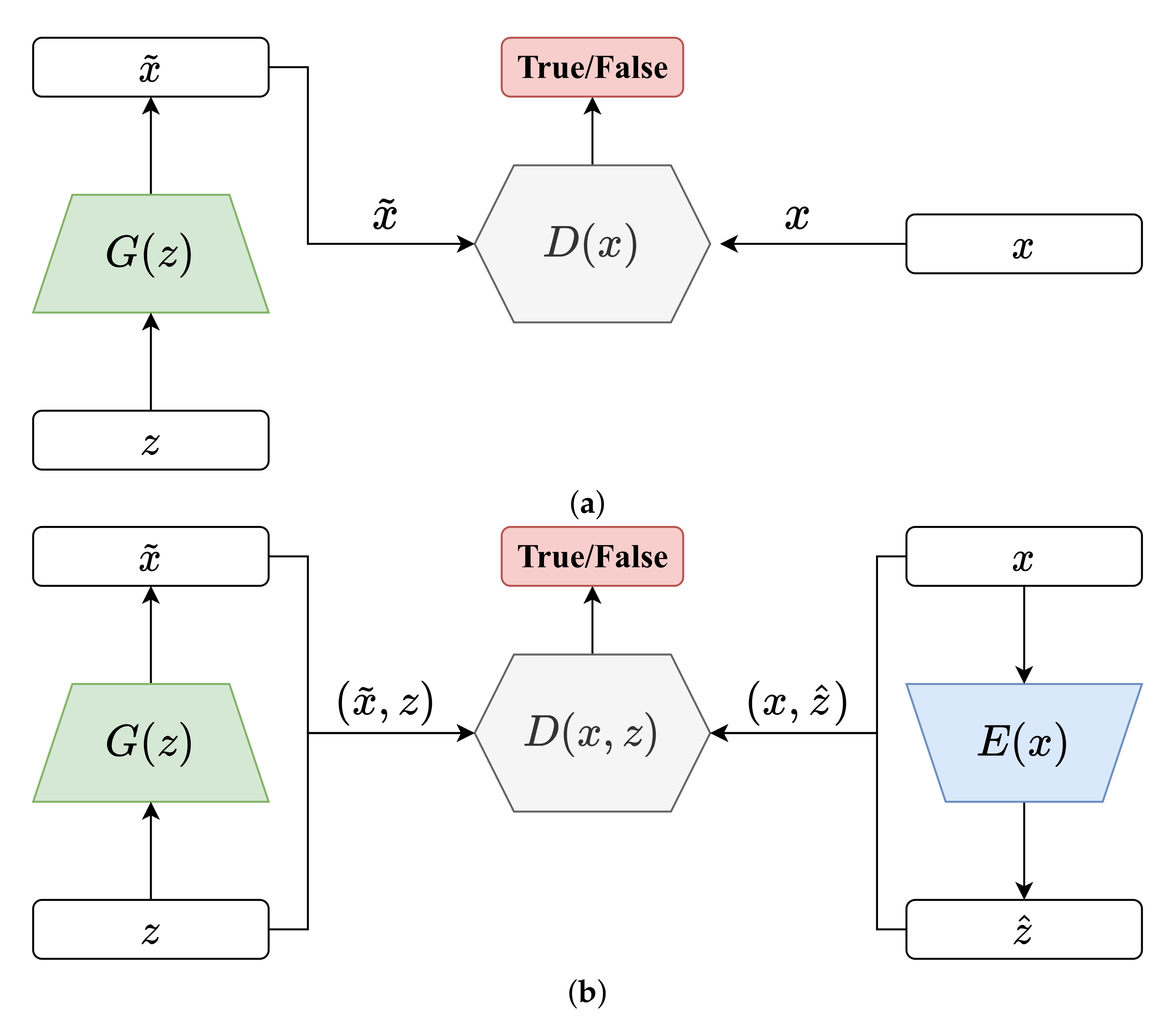
Adequate epochs of training are necessary to learn the pattern of real data. However, the number of the unsupervised training epochs is not the more the better. To determine the appropriate number of training epochs, an experiment is designed. First, during the unsupervised pre-training, we saved the parameters of the encoder every 100 epochs. So, pre-trained models with different training epochs can be obtained. Then, fine-tuning is conducted on the saved models using the same labeled training set. Finally, the models are tested on the same testing set. Figure 4a shows the trend of diagnosis accuracy through the pre-training process. It shows that the accuracy increases rapidly at the beginning and then decreases as the number of training epochs increases. Figure 4b shows the loss of pre-training and fine-tuning with increasing pre-training epochs. The overall trend of the loss of pre-training is decreasing, but the loss of fine-tuning decreases at the beginning and then increases, which supports the trend of accuracy. Therefore, pre-training epochs around 2300 may be appropriate. One possible reason is that since the generator and encoder are optimized at the same time, an overfitting phenomenon similar to that when the autoencoder is over-trained may have occurred, resulting in a degradation of the encoder’s feature representation capability.

4. Experimental Verification

To verify the performance of the proposed method, two experiments are designed in this section: data generation and fault diagnosis. The proposed method is verified on two types of basic rotating machinery: bearing and gear.

4.1. Datasets Description

4.1.1. CWRU Bearing Fault Dataset

The bearing fault dataset of Case Western Reserve University (CWRU) Bearing Data Center [25] is one of the most widely used datasets in the field of fault diagnosis. This dataset collects data from a ball bearing on a test rig, which is driven by a 2 hp Reliance electric motor, and accelerometers are used to record vibration data of the bearing at the motor drive end. Using electro-discharge machining (EDM) technology, artificially created defects ranging from 0.007 inches (0.1778 mm) to 0.028 inches (0.7112 mm) in diameter located in the inner race, outer race, and rolling elements of the bearing. And vibration data is recorded for motor loads of 0 to 3 horsepower (speed 1797 rpm to 1720 rpm). The torque sensor and encoder are used to record the load and motor speed, respectively.

This article uses bearing vibration data at the drive end of the motor. As shown in

Table 2. CWRU bearing dataset faults.

Category	Condition	Defect Diameter (Inch)	Label
1	Normal	-	Normal
2	Inner race	0.007	IR07
3	Inner race	0.014	IR14
4	Inner race	0.021	IR21
5	Rolling elements	0.007	RE07
6	Rolling elements	0.014	RE14
7	Rolling elements	0.021	RE21
8	Outer race	0.007	OR07
9	Outer race	0.014	OR14
10	Outer race	0.021	OR21

, a total of 10 types of working conditions are used as classification categories, including one normal and 11 fault conditions. We use the fault data at a 12 kHz sampling rate, and the 48 kHz normal data is resampled to 12 kHz to ensure the consistency of data. First, by splitting the original data into segments of 1024 data points in the time domain, we obtained a dataset of 1000 samples for each category, for a total of 10,000 samples. Then, Fast Fourier transform (FFT) is used as a data preprocessing method to obtain frequency domain signals, and the magnitude of each sample is normalized into [0,1]. Additionally, to avoid the effect of spectral leakage, a Hamming window function is applied for each segment of the signal before FFT. Finally, due to the symmetry of the FFT results, we usually use only the first half of the results, so the length of each sample is 512 eventually.

4.1.2. UoC Gear Fault Dataset

According to a benchmark study [26], the CWRU bearing fault dataset is relatively easy to diagnose. However, the University of Connecticut (UoC) gear fault dataset [27,28] is a challenge for many classical models such as autoencoder (AE) and CNN. Therefore, we use the UoC gear fault dataset to further evaluate the proposed method on different types of rotating machinery.

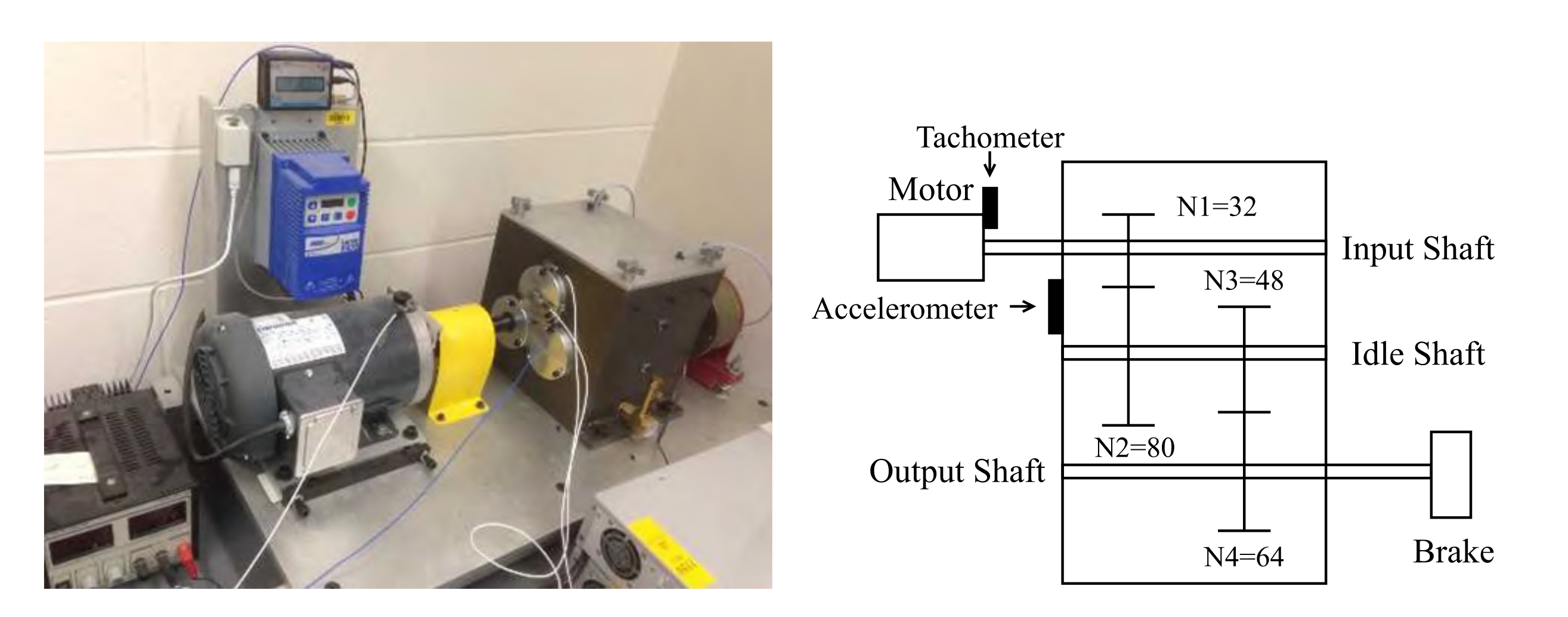
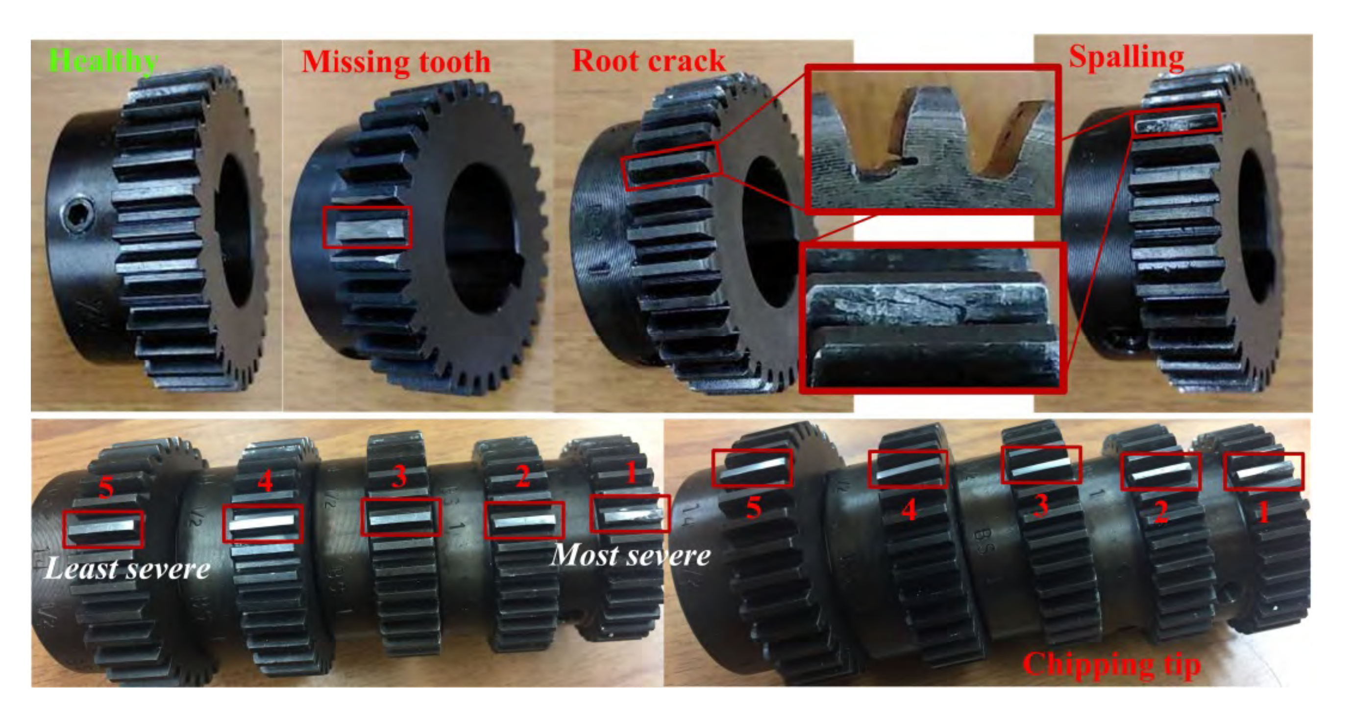
As shown in Figure 5, the two-stage gearbox is driven by an electric motor. The first stage consists of a 32-tooth pinion on the input shaft and an 80-tooth gear, and the second stage consists of a 48-tooth pinion and a 64-tooth gear. A magnetic brake is connected to the output shaft as the load. By replacing the pinion on the first stage input shaft, nine different working conditions are introduced into the system, including healthy condition, missing tooth, root crack, spalling, and chipping tip with five different levels of severity, as shown in

Table 3. UoC gear dataset faults.

Category	Condition	Severity	Label
1	Healthy	-	HT
2	Missing tooth	-	MT
3	Root crack	-	RT
4	Spalling	-	SP
5	Chipping tip	1	CT1
6	Chipping tip	2	CT2
7	Chipping tip	3	CT3
8	Chipping tip	4	CT4
9	Chipping tip	5	CT5

and Figure 6. An accelerometer is used to record the original vibration signals of the gears with a sampling frequency of 20 kHz, and 104 samples are recorded for each working condition, each sample containing 3600 data points.

As same as the CWRU dataset, we split the original data into segments of 1024 data points in the time domain, then FFT and standardization are performed. Eventually, the gear dataset consists of 312 samples for each category, for a total of 2808 samples.

4.2. Data Generation Experiment

Data generation is an effective application of GAN that helps to solve the problems such as lack of training samples and data imbalance. As a GAN-based model, BiWGAN-GP is also capable of generating data. Besides, a good generation result also means good feature extraction capability of the encoder [19]. Therefore, this experiment is designed to evaluate the quality of generated data.

For comparison, the origin GAN, WGAN, WGAN-GP, BiGAN, and improved BiWGAN-GP models are trained to generate vibration signals in the frequency domain. All models have the same structure of generator. The BiGAN and BiWGAN-GP have the same architecture but only different loss functions for training. The models are trained for 2000 epochs using all of the available unlabeled data. After training, 1000 unlabeled samples are generated by feeding forward random noise into the model’s generator.

(1) Quantitative assessment: To quantitatively evaluate the generated data of GAN, inception score (IS) [29] and Fréchet inception distance (FID) [30] are popular evaluation metrics. However, those methods are designed for image generation tasks, and unsuitable for vibration signals. In this paper, maximum mean discrepancy (MMD) [31] and Pearson correlation coefficients (PCC) are used to quantitatively assess the quality of generated data. The MMD can be calculated directly between two sets of samples. And the PCC is used to assess the linear correlation between two specific signals. With these two methods, we can evaluate the generation effect on two different scales.

Table 4. Quantitative assessment results of the generation quality.

	CWRU Dataset		UoC Dataset
	MMD	PCC	MMD	PCC
GAN	2.5757	0.5307	0.2706	0.8482
WGAN	0.3052	0.7640	0.1960	0.8642
WGAN-GP	0.0334	0.8270	0.0215	0.8898
BiGAN	2.0498	0.6101	0.2393	0.8557
BiWGAN-GP	0.0226	0.8277	0.0221	0.8917

shows the MMD and average PCC between generated data and real samples. The lower MMD means better generative result, and the closer the PCC is to 1 means the more similar the two samples are. The results on the CWRU dataset show that GAN and BiGAN have relatively higher MMD and lower PCC, and BiGAN is slightly better. With the help of Wasserstein distance, the MMD of WGAN is lower than GAN and BiGAN and the result of PCC has also improved. The results of WGAN-GP and BiWGAN-GP are much better than the other methods, which suggests that Wasserstein distance with generation quality effectively improves the model’s generative capability. Furthermore, the differences between WGAN-GP and BiWGAN-GP are minor, implying that their generation capabilities are similar. As for the UoC gear dataset, the numerical difference between the various models is smaller than the results on CWRU dataset. However, the generation effect reflected in the result is similar. Although WGAN-GP reached the best MMD in the UoC dataset, the gap between BiWGAN-GP and WGAN-GP is minor. Overall, BiWGAN-GP achieves the best quantitative assessment results.

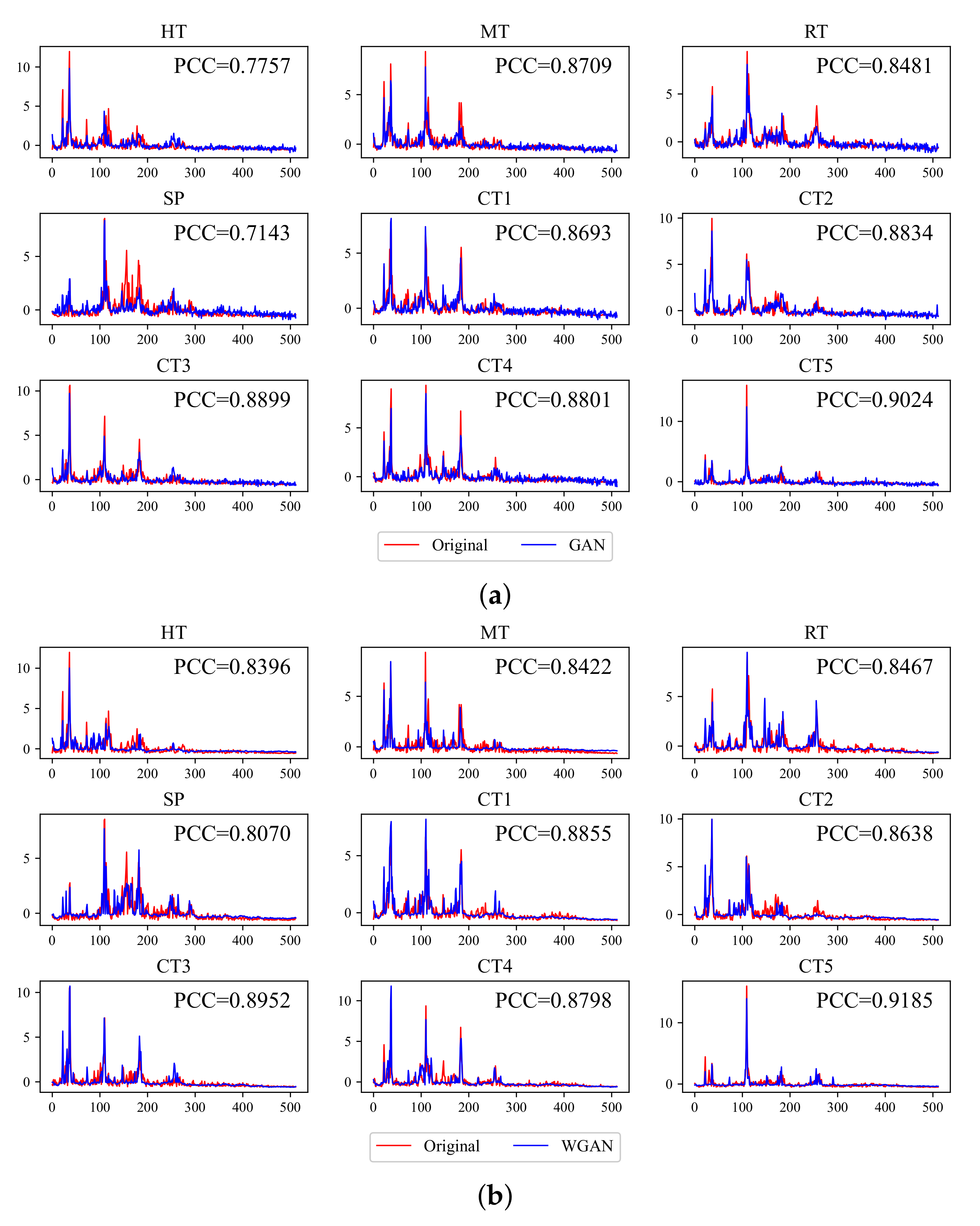
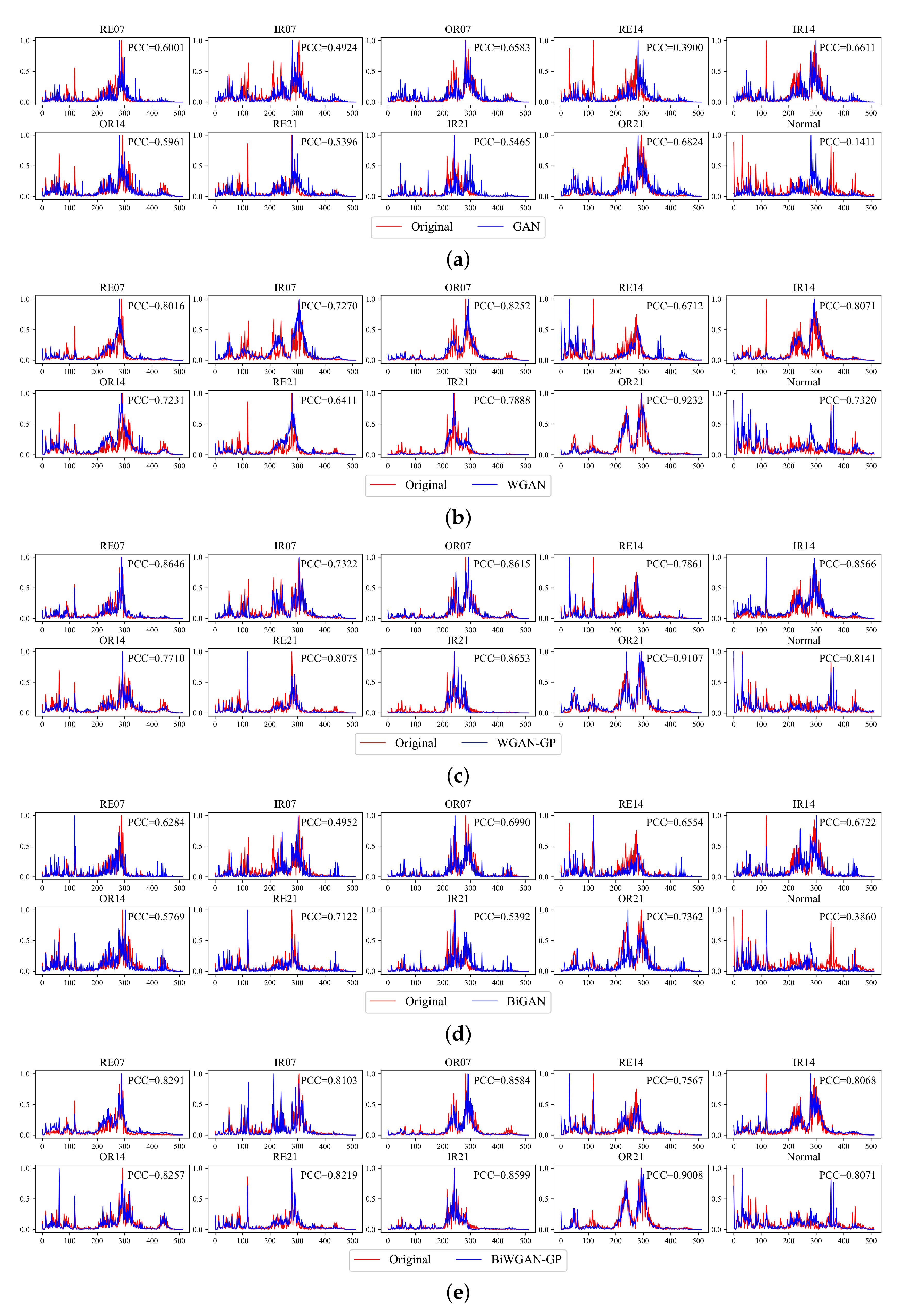
(2) Visualized assessment: To visualize the quality of generated results, we show the comparison between the original and generated frequency spectrum of the CWRU dataset in Figure 7. For clarity, the comparison of the UoC dataset is shown in Figure A1 in Appendix A. Since the generator is trained unsupervisedly, the generated data is also unlabeled. Therefore, by iterating through the generated samples, we find the sample that is most similar to each category, i.e., samples with the smallest mean square error to original signals. The PCC between the generated and original signal of a specific category is shown in every subfigure.

The visualization supports the results of the quantitative assessment. Figure 7a,d show that mode collapse is evident in GAN and BiGAN, which should be the main reason for their higher MMD. It is noticeable that some significant frequency points in the origin are missing, but lots of unexpected spikes show up. Figure 7b shows that WGAN does not have mode collapse, but it seems to have a filtering effect that tends not to generate spikes, which also causes the error between the generated and real samples. It may be caused by gradient clipping in WGAN. In contrast, Figure 7c,e show that the difference of signals generated by WGAN-GP and BiWGAN-GP is difficult to distinguish, which is consistent with the results in the quantitative assessment. The features of the original spectrum are well-matched in the generated signals. Figure A1 shows that the generative results of the UoC dataset are relatively hard to distinguish by human eyes. However, we can tell that the signals generated by GAN and BiGAN have some meaningless fluctuations in the high-frequency part and some spikes in the gear spalling fault are missing. The results of WGAN-GP and BiWGAN-GP are better than others, and the PCC also confirmed it. The results suggest that Wasserstein distance with gradient penalty seems to be indispensable to improve the generation quality.

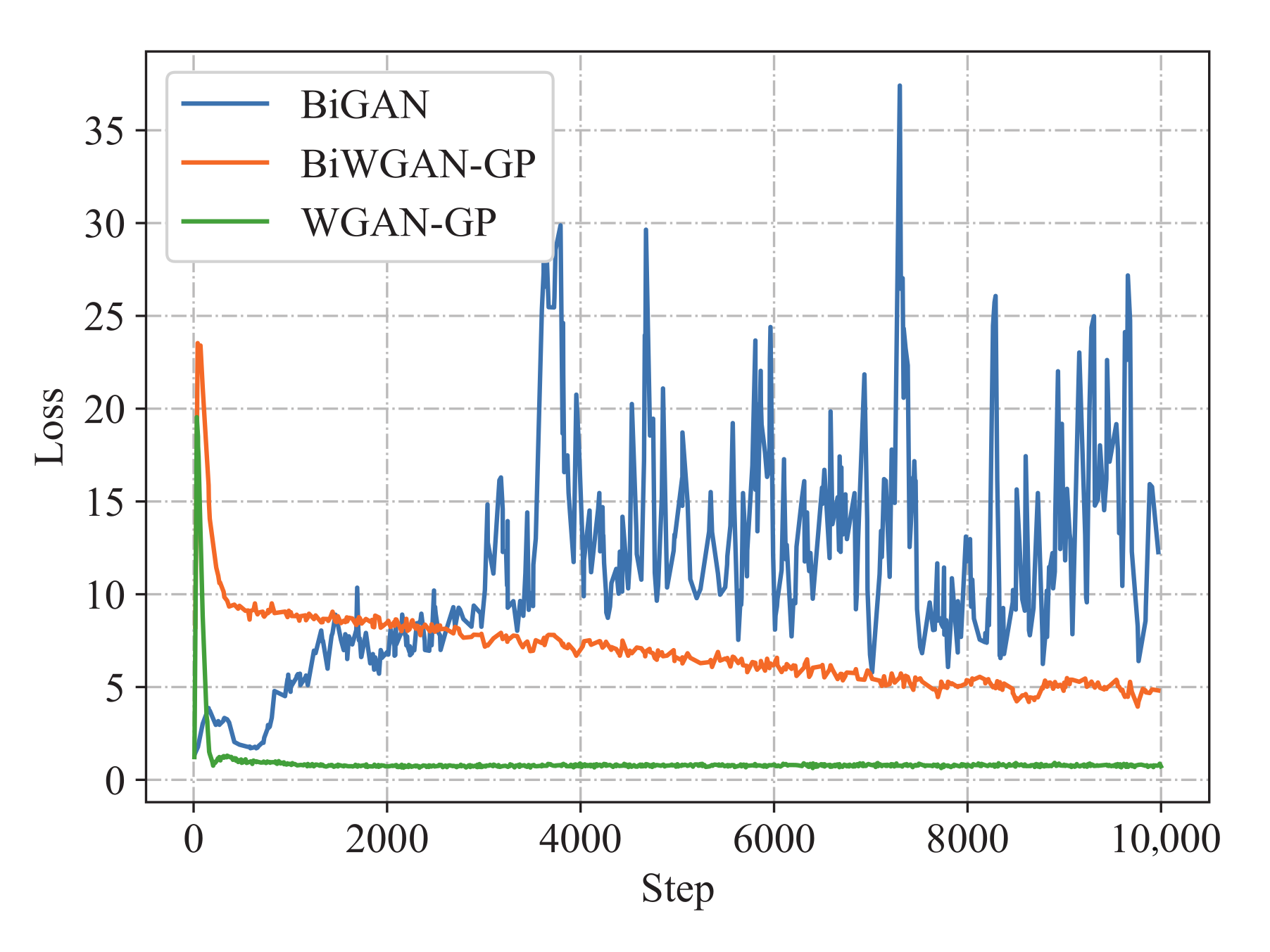
(3) Analysis of the training loss: The trend of training loss may explain the difference in model generation quality. Losses are recorded during the unsupervised pre-training stage. Figure 8 shows the training loss of generator G and encoder E of BiGAN and BiWGAN-GP, and the training loss of generator G of WGAN-GP. The results show that the loss of BiGAN has an unstable trend. Under the same training conditions, BiWGAN-GP shows a different result, that the loss of E and G (also means the Wasserstein distance) decreases steadily. The loss values of WGAN-GP are much lower than those of BiWGAN-GP, but the numerical comparison between them is meaningless because of the missing encoder and the different discriminator structures. It is worth noting that they both have a steady trend. These curves demonstrate that the stability of BiWGAN-GP’s training is much improved and also explain why the generative ability of BiWGAN-GP is better than BiGAN.

4.3. Fault Diagnosis Experiment

To verify the fault diagnosis performance of the method proposed in this paper, a comparative experiment is conducted in this section. Four semi-supervised fault diagnosis methods are compared: original BiGAN [19], denoising autoencoder (DAE) [32], variational autoencoder (VAE) [33], and proposed BiWGAN-GP.

(1) Experiment setup: These methods have similar usage for fault diagnosis tasks, including unsupervised pre-training and supervised fine-tuning. First, all methods use the same amount of unlabeled data for pre-training, which allows the model to perform effective feature extraction. Then, the encoder is picked out from the model as a feature extractor. To evaluating the model’s unsupervised learning ability, the encoder’s parameters are frozen to prevent being trained in the next stage. After adding a linear classifier layer, supervised fine-tuning is conducted using different amounts of labeled data as the training set. Since the main idea of this experiment is to evaluate the model’s performance with insufficient labeled training data, the training set is smaller than the testing set. The number of testing samples of the CWRU and UoC dataset is 4000 and 900, respectively, and the number of training samples is set to 1%, 5%, and 10% of the testing set. Specifically, there are 40, 200, and 400 training samples of the CWRU dataset, and 9, 45, 90 training samples of the UoC dataset.

(2) Comparison of the diagnosis accuracy:

Table 5. Comparison of diagnosis accuracy(%) on different size of training set.

Method	Number of Labeled Training Samples
	CWRU Dataset			UoC Dataset
	40	200	400	9	45	90
DAE	94.65	97.78	98.74	38.82	73.96	84.23
VAE	79.95	89.06	94.30	37.74	75.56	81.22
BiGAN	74.22	84.86	92.09	48.04	53.26	55.33
BiWGAN-GP	97.14	99.21	99.42	51.07	85.70	91.97

shows the comparison of average diagnosis accuracy under the various size of the training set. Under the same condition of training samples, the proposed method has significantly higher accuracy than others, which implies that the BiWGAN-GP can benefit more from the unsupervised training. Additionally, the BiWGAN-GP’s result is much better than BiGAN’s, which indicates the improvements are necessary and effective. Compare to the CWRU dataset, the UoC gear fault diagnosis task is relatively harder, therefore the average accuracy of the UoC dataset is lower, but the proposed method also reaches an acceptable result. The results demonstrate that the amount of labeled data is a direct factor in the accuracy. However, when the available labeled data is lacking, the feature representation ability obtained from unsupervised training is the crucial factor of diagnostic accuracy.

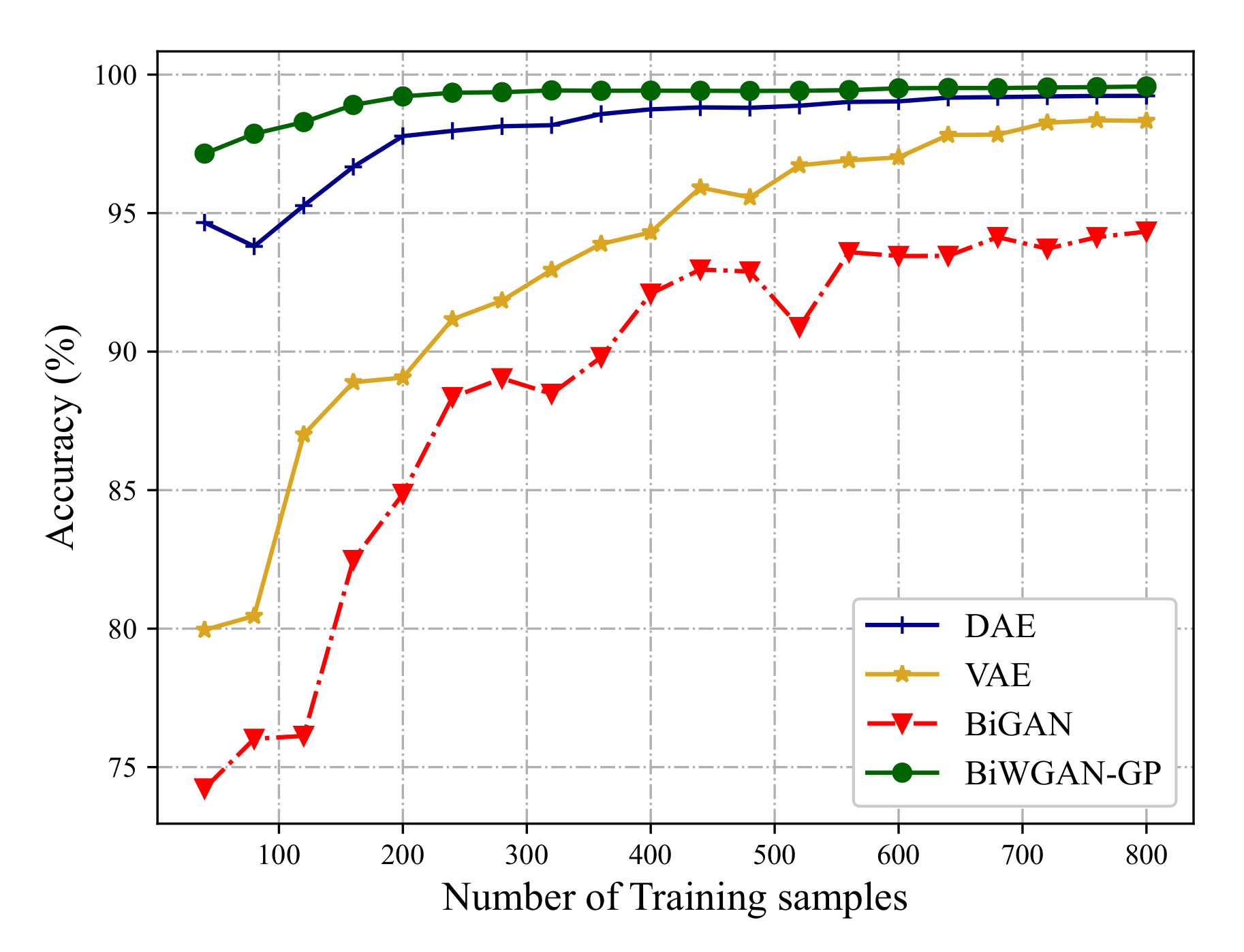
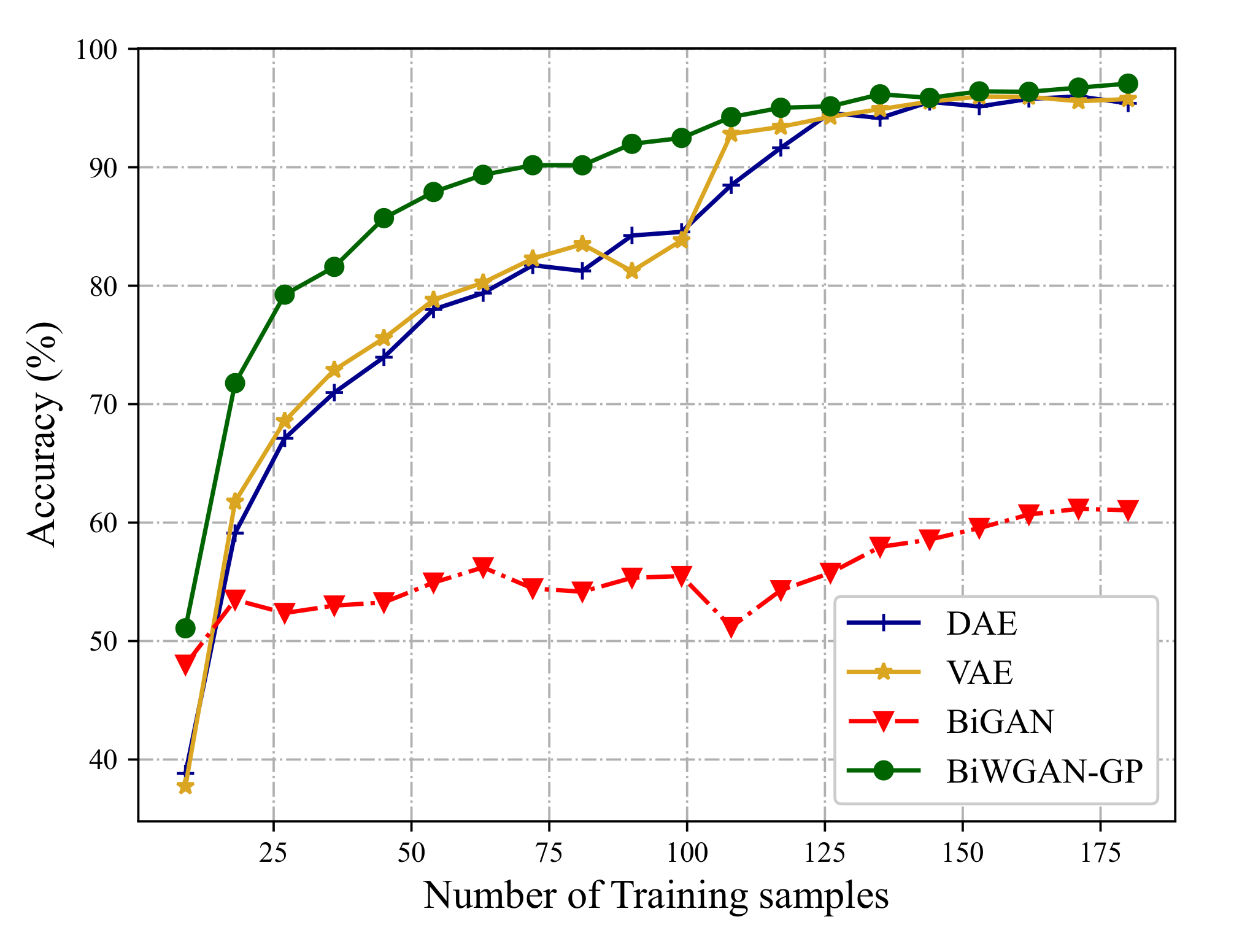
To show the comparison more clearly, accuracy curves are plotted by increasing the number of training samples from 1% to 20% of the testing set. Figure 9 and Figure 10 plot the accuracy curves on the CWRU dataset and UoC dataset, respectively. The results show that on the condition of insufficient labeled data, the proposed method can provide reliable fault diagnosis. Meanwhile, the increase of accuracy from BiGAN to BiWGAN-GP proves the effectiveness of the improvement in Section 2.3.2. It also can be concluded that more labeled data make better diagnosis performance, which partly explains why many previous works can achieve very high accuracy on fault diagnosis. With labeled data increasing, the performance difference between BiWGAN-GP and other methods decreases, but BiWGAN-GP is still better than others.

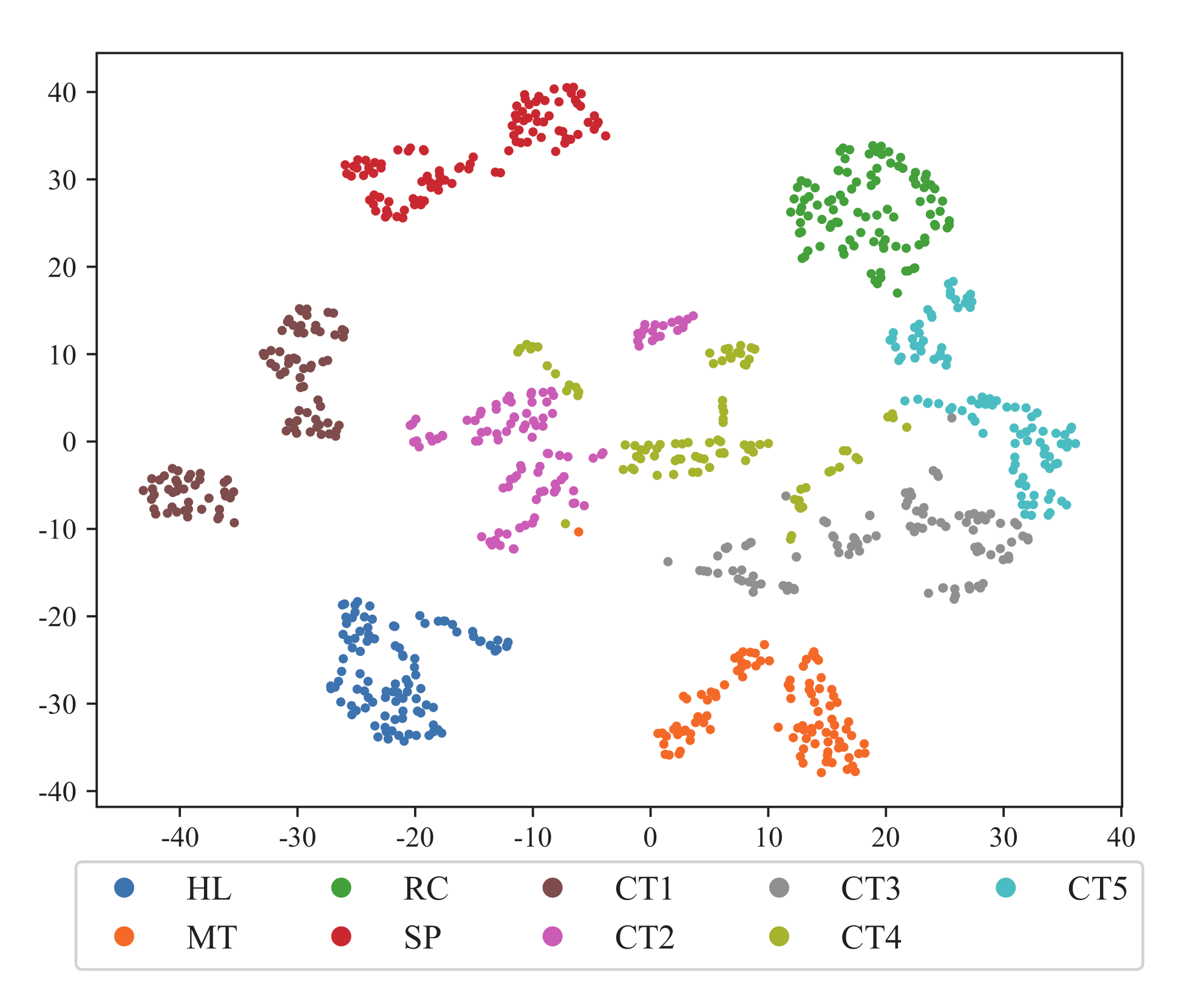
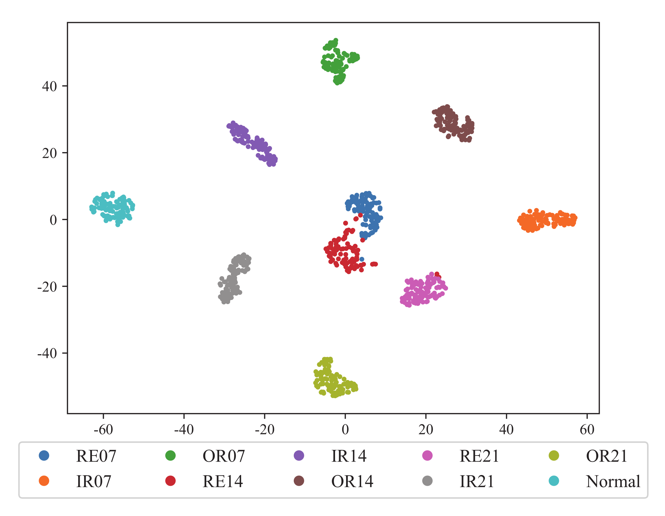
(3) Visualization of the extracted features: To further evaluate the feature learning ability of BiWGAN-GP, the extracted features are visualized using t-SNE [34]. Figure 11 shows the dimensional reduction result of the features extracted by the encoder of BiWGAN-GP on the CWRU dataset. Different color represents the category of working condition, and the label’s meaning is as shown in Table 2. The result shows that different types of faults can be easily separated into clusters, which implies the good performance of the model’s encoder. Figure 12 shows the visualization of feature extraction of the UoC dataset, and the scatter shows a similar result.

5. Discussion

The above experiment verifies that the proposed method can generate real-like vibration signals and perform accurate semi-supervised fault diagnosis. The task of generating vibration signals shows that although Wasserstein distance can solve the mode collapse problem, gradient clipping will cause distortions, and the gradient penalty can restore the original signal pattern. It indicates that the improvements of the loss function of the GAN-based model are still worthy of thorough exploration. The fault diagnosis experiments demonstrate that although the number of labeled samples is an essential factor in the performance of the semi-supervised learning model; the utilization of unlabeled samples also has a significant impact on diagnostic accuracy. Therefore, using a large amount of unlabeled data more efficiently to improve the performance of the fault diagnosis methods is worthy of further investigation. In addition, it should be pointed out that currently available public datasets in the field of fault diagnosis are limited. More and various public datasets will help the development of the predictive maintenance community.

6. Conclusions

This article proposes a novel semi-supervised machinery fault diagnosis method called BiWGAN-GP. The proposed method utilizes the information of available unlabeled data effectively and reduces the model’s need for the amount of labeled data, which can save the cost of manually labeling data. By using the Wasserstein distance to improve the training procedure, the model can be trained stably and reliably. The experiments show that the proposed method can generate real-like signals using unlabeled data which is easy to obtain, and also can perform accurate fault diagnosis using only a few labeled data. Furthermore, the structure of BiWGAN-GP is simple to modify. By replacing the fully connected layers with a one-dimensional convolutional layer, the model is capable to deal with the generation and diagnosis tasks of the raw time-domain signals.