An Improved Seismic Vulnerability Assessment Approach for Historical Urban Centres: The Case Study of Campi Alto di Norcia, Italy

Abstract

Seismic damage assessment is an extraordinary opportunity to evaluate the reliability of vulnerability and risk methodologies applied to historic masonry buildings, giving the possibility of enhancing and optimising mitigation and retrofit strategies. Vulnerability index methodologies are flexible and powerful tools for assessing seismic vulnerability on the urban scale, providing a first screening of the critical issues present in masonry buildings and a possible priority list for the following retrofit operations. Such approaches account for the buildings’ different structural characteristics, directly or indirectly influencing their seismic behaviour and measured through different weights and classes finally providing a vulnerability index. In this paper, we show the application of three well-known methodologies to Campi Alto di Norcia’s medieval city in Valnerina (Italy) stroke by the earthquakes of 24 August and 30 October 2016. The methodologies’ reliability is assessed, based on the observation of real seismic consequences and damages on the masonry buildings, and an optimised methodology is then proposed for the considered case study.

1. Introduction

Heritage buildings are the result of an interaction process between people and the surrounding area: the heterogeneous architecture of ancient city centres is the direct expression of cultural modifications, natural transformations and anthropic events occurred over the centuries. The masonry buildings constituting the urban environment are usually organized within structural aggregates (SAs), not following a regular development and therefore resulting in different construction typologies influenced by the materials available in the territory, regional traditions and realization periods. SAs are typically made up of buildings—recognized as “structural units” (SU)—connected in a variety of different ways, leading to different geometric configurations. The structural performance of the SAs is influenced by every single SU constituting it, which are often characterized by heterogeneous structural features, materials and architectures [1].

The morphological variety of the resulting urban settings enriches the cultural heritage of a place, but, in the meanwhile, increases local and global vulnerabilities towards static and seismic actions, due to the lack of connections between structural elements of masonry buildings. Recent earthquakes that stroke Italy during the last decades have [2] highlighted failures of masonry aggregates caused by the activation of local mechanisms, not allowing the development of global building behaviour [3,4,5], together with the negative impact of past retrofit interventions that frequently increased vulnerabilities instead of reducing them [6]. The implementation of seismic prevention and retrofit strategies for historical city centres requires the knowledge, on a territorial scale, of the risk to which existing SAs are exposed [7], of the adopted materials, structural features, morphological evolution of the aggregates and, above all, of the interaction between SUs and SA during the earthquake.

Being the seismic risk is the combination of structural vulnerability, exposure and seismic hazard, the analysis of each of the three parameters mentioned above becomes a relevant issue for the global understanding of the state-of-the-art of a historical construction or SA. Several methods exist in the current scientific literature for the vulnerability assessment of masonry aggregates in historical city centres, based on a multi-level approach characterized by increasing knowledge and in-depth in-situ evaluations [8]. Among them, the simplest approaches are known as statistical (or observational) methods; they can be used for a quick and easy analysis of seismic risk at regional/urban scale by defining, for each masonry construction, a vulnerability index (I_V) accounting for different parameters whose weight is assumed based on expert evaluations of the post-seismic damage conditions [9]. The statistical approach allows to summarize the observed damages and the results of in-situ investigations through damage probability matrices (DPMs), analysing vulnerabilities and estimating damage for different structural typologies [10,11]. Statistical methods are powerful tools for providing a preliminary screening of constructions’ fragilities on the territory, determining a sort of priority list for the execution of deeper investigations and for the following planning of retrofit interventions. Their limit otherwise lies in the constructions’ scenario to which they can be applied: their reliability progressively decreases when applied to structures considerably different respect to the ones used for the method’s calibration [12]. In addition, the lack of information coming from a survey may overlook critical epistemic uncertainties, influencing the results [13,14]. Since these methods are applied through external onsite inspections, the level of confidence concerning the geometric composition, the material properties, the boundary conditions and loads involved among the orthogonal walls of the construction analysed, depends on the available data and the experience of the technician [13,15,16,17,18]. In this context, Cosenza et al. (2005b) [19] try to solve this kind of uncertainties with similar procedures but regarding RC buildings, which are more standardized.

A more detailed analysis’ possibility consists of adopting mechanical methods describing the SU’s structural performance and the resulting seismic vulnerability of the SA through in-depth numerical modelling and assessment. Despite the accuracy of the achieved results, sophisticated modelling tools are needed to simulate the nonlinear behaviour of masonry structures subjected to lateral loading [15,16] leading to a strong computational and time effort and, besides, to difficulty in the interpretation of data. Moreover, detailed modelling guidelines for the evaluation of the connections between SAs are missing [17], and the reliability of mechanical methods decreases for areas with varied construction typologies, built with different materials [18,19]. Therefore, it is difficult to use mechanical methods for a quick and easy analysis of seismic risk at regional/urban scale, being their application more efficient for single buildings in aggregates [20].

The aim of the present research work was the development of an enhanced statistical method for the seismic vulnerability assessment of masonry aggregates and, in general, of historical city centres characterized by high cultural and historical value actually not provided by adequate analysis’ tools for achieving large-scale reliable results. The proposed methodology adopts a multi-step approach owning the advantage of being calibrated basing on the damages observed in the post-earthquake event phase of Central Italy (2016): this makes the proposed method reliable for a variety of construction typologies widespread on the territory in Central Italy, reducing the error connected to the application of traditional literature approaches. The calibration procedure was developed considering the case study of Campi Alto di Norcia (Italy), hit by an earthquake with a specific intensity. Then, mathematical methods allow extending the achieved results to seismic events of other intensities, defining different possible damage scenarios. In addition, comparing with other methods presented in the literature—some of them will be addressed herein [21,22,23], the proposed one accounts for the lack of information about specific parameters—by introducing an Information Quality (IQ) index—and for the influence coming from the experience of the technician performing the survey in evaluating the vulnerability index.

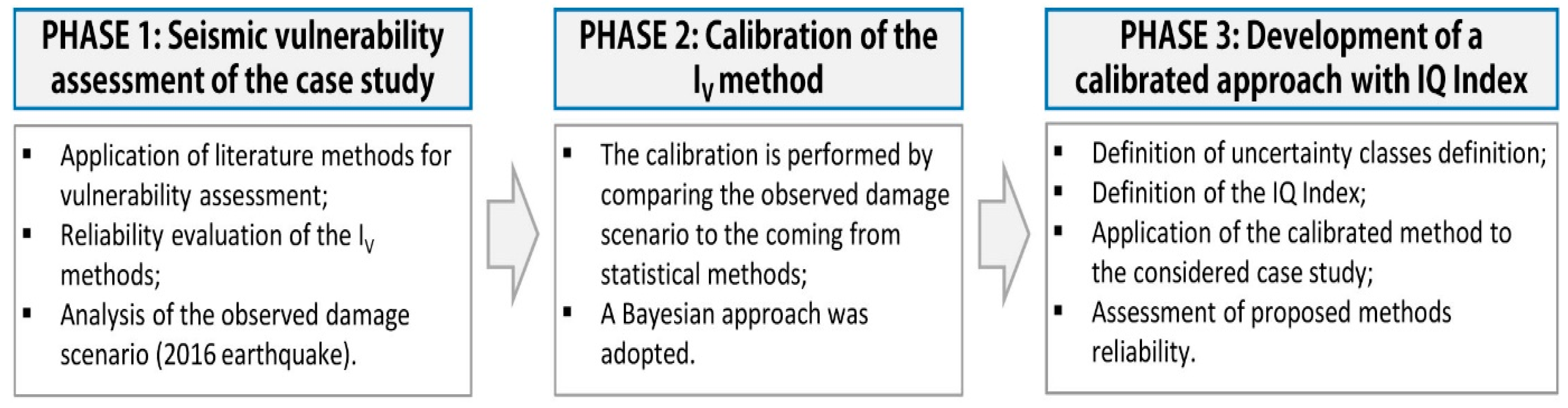
2. Research Methodology

The methodology adopted in the present research work can be summarized in the following phases (Figure 1), described with more details in the following paragraphs.

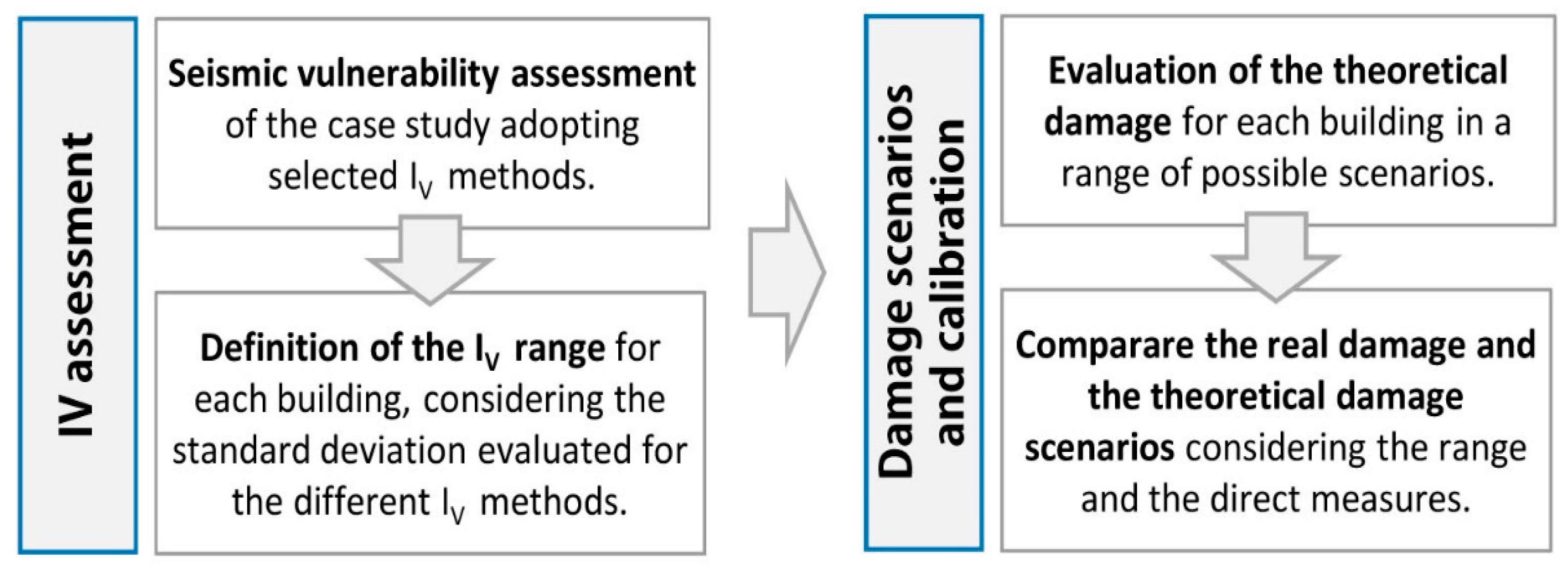
• Phase 1: Seismic vulnerability assessment of the case study. Different statistical methods were selected and applied to Campi Alto di Norcia (Italy) with the aim of determining the corresponding I_V and comparing their accuracy in predicting the damage scenarios. Possible limitations of selected methods were highlighted, finally selecting the most performing one for the considered case study. A database of information with data coming from in-situ surveys was elaborated.
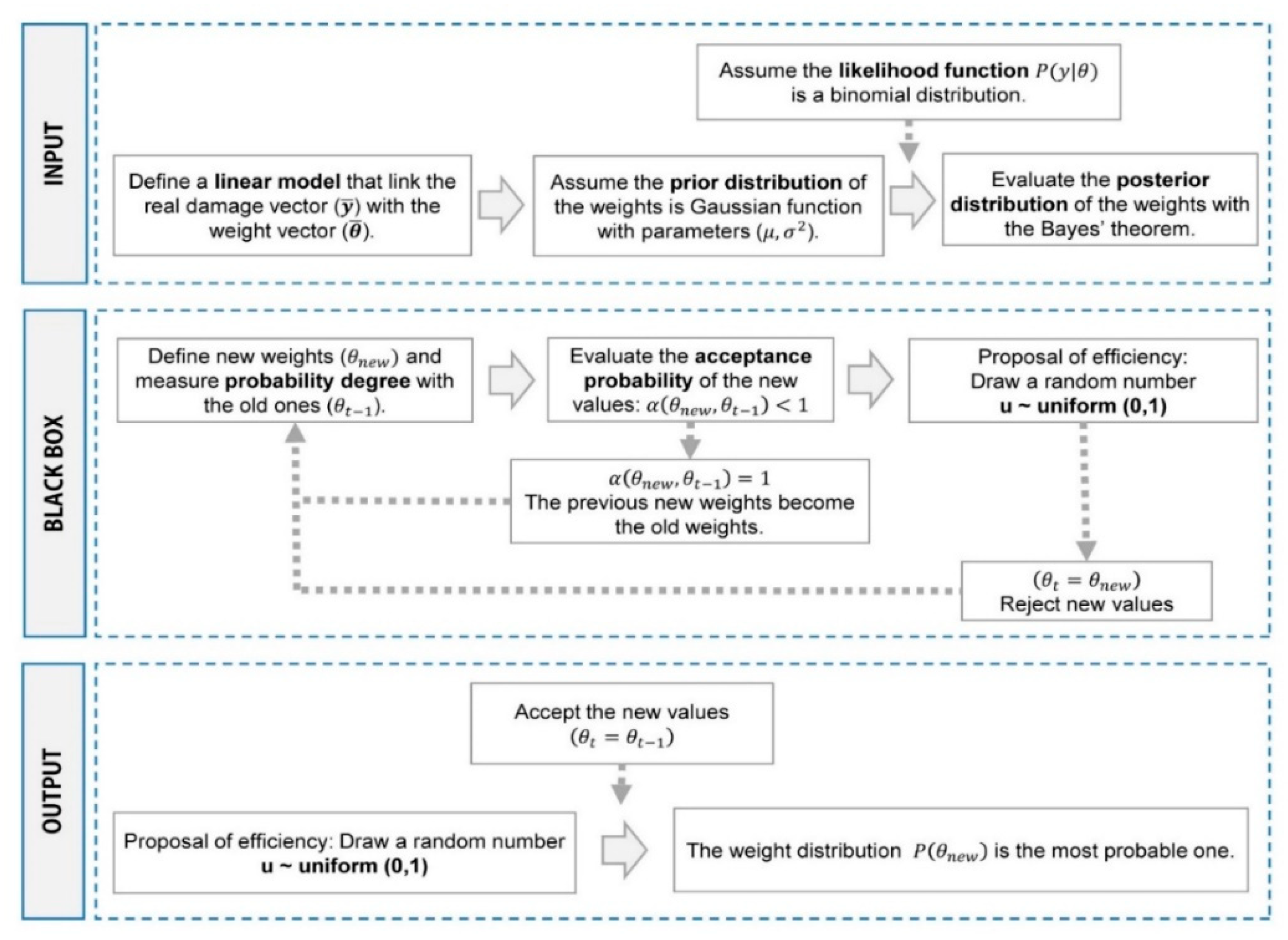
• Phase 2: Calibration of the I_V method. Based on the achievements of Phase 1, the calibration of the adopted vulnerability index method for the selected case study was performed, by comparing the “observed” damages caused by the 2016 earthquake with the “analytical” ones predicted through the previously selected method. The calibration was carried out through a statistical analysis within the context of Bayesian inference [24].
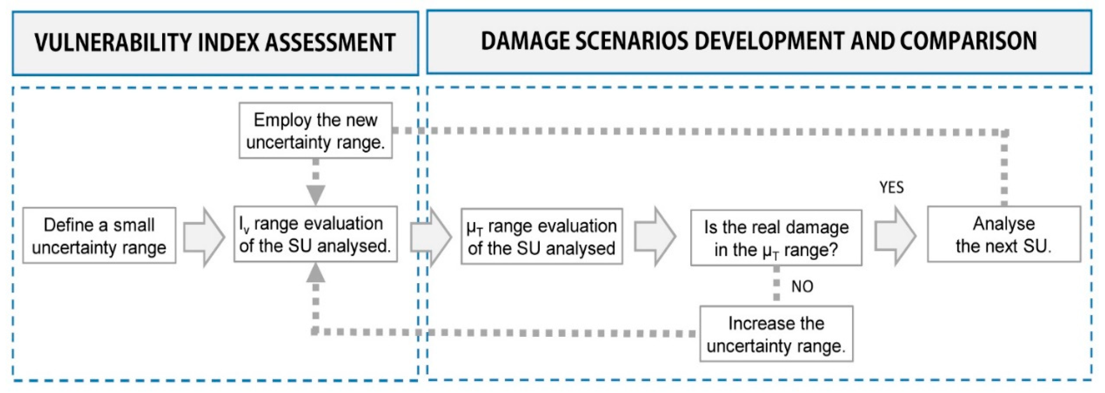
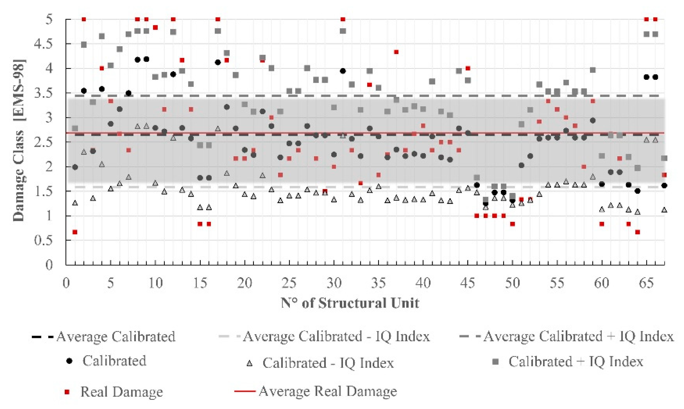
• Phase 3: Development of an enhanced approach with the IQ index. An additional IQ index was introduced in the calibrated procedure (Phase 2) accounting for uncertainties related to the lack of information due to limited access or inspections. The knowledge uncertainty was quantified through a parameter measuring its influence in the final vulnerability assessment; an iterative analysis involving the change of the uncertainty range of the parameters based on the observed damages was adopted.

3. The October 2016 Seismic Crisis

The 2016 October seismic crisis involved a series of seismic events that affected a large area of Italian territory located along the central Apennines, between the Region of Lazio (L), Umbria (U), Marche (M) and Abruzzo (A), from August 2016 to January 2017. The earthquake characteristics are expressed in terms of magnitude, in order to have an overall measure of the energy released during the seismic crises.

The first strong earthquake occurred on 24 August (Mw = 6), with the epicentre positioned in the Tronto Valley, between the historical centres of Arquata del Tronto (M) and Accumoli (L) [25]. The village of Amatrice was utterly destroyed, causing hundreds of casualties and people left injured and homeless. During the earthquake swarm, two strong aftershocks took place: the first on 26 October (Mw = 5.9) with epicentre in the Umbria–Marche borders, between the villages of the province of Macerata di Visso (M), Ussita (M) and Castelsantangelo sul Nera (M), while a second on 30 October (Mw = 6.5) with epicentre between the cities of Norcia (U) and Preci (U) [26]. This last event caused the collapse of several buildings and above all churches in a wide area, such as the basilica of San Benedetto in Norcia and San Salvatore’s church in Campi Basso. The events of 26 and 30 October did not cause any casualties in Campi Alto di Norcia, because residents were evacuated from the city immediately after the previous seismic events. Other aftershocks took place in January 2017 with a lower magnitude.

Table 1. Parameters of the main seismic events of the earthquake swarm.

Earthquake Date (yyyy–mm–dd)	Origin Time (UTC)	Magnitude (Mw)	Epicentre Area	Hypocentral Depth (Km)	Latitude (N°)	Longitude (E°)
2016 08 24	01:36:32	6.0	Accumoli (L)	8.0	42.70	13.23
2016 08 24	02:33:28	5.4	Norcia (U)	7.5	42.79	13.15
2016 10 26	17:10:36	5.4	Visso (M)	8.7	42.88	13.13
2016 10 26	19:18:05	5.9	Visso (M)	8.0	42.91	13.13
2016 10 30	06:40:17	6.5	Norcia (U)	9.0	42.83	13.11
2017 01 18	10:14:09	5.5	Montereale (A)	10.0	42.53	13.28
2017 01 18	10:25:23	5.4	Montereale (A)	9.0	42.49	13.31

shows the evolution of the 2016–2017 earthquake sequence, identifying the position of all the mainshocks and the epicentre areas.

The main shocks, that occurred in Campi Alto between 26 and 31 October 2016, are extrapolated from the earthquake’s strong ground motion and post-processed.

Table 2. Max PGA (% g) recorded by the accelerogram of the Campi Station in the three main directions for different seismic events. The minus signs of the last column highlight the upward seismic acceleration.

Earthquake Date (yyyy–mm–dd)	Origin Time (UTC)	Magnitude (Mw)	East–West (pga)	North–South (pga)	Up–Down (pga)
2016 10 26	17:10:36	5.4	0.713	0.341	−0.429
2016 10 26	19:18:06	5.9	0.644	0.308	0.489
2016 10 31	07:05:45	4.0	0.180	0.087	−0.083

shows the maximum peak ground acceleration (PGA) registered by the Campi station for the different seismic events analysed. It is not correct to compare single PGAs with forecasted shakings (PGA with 10% probability of exceedance in 50 years), since probabilistic models cannot be validated (or rejected) on the basis of a single event, but this process is useful to understand the consistency of the model suggested by the Italian Code [27]. In this sense, the maximum PGA is much higher than the one generally used for the structural analysis of the buildings located in this area and, therefore, provide important information about the action to which the structures were subjected and the resulting damage.

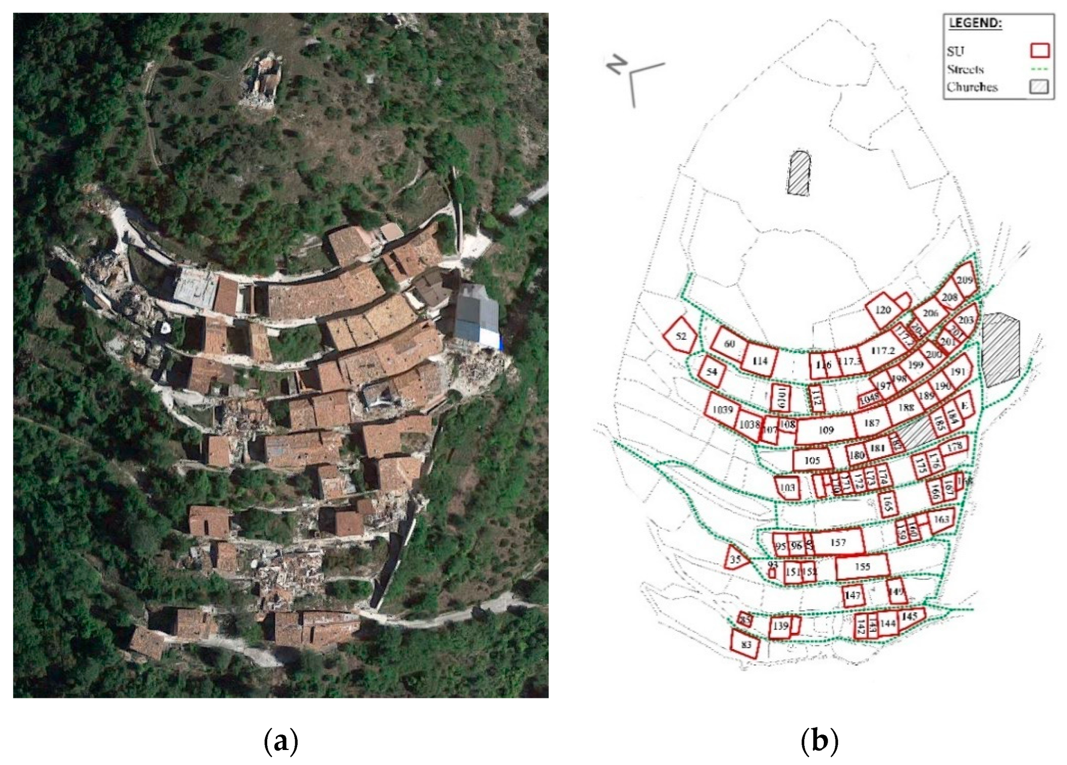
4. Campi Alto di Norcia: Description of the Historical City Centre

The selected case study city centre is Campi Alto di Norcia’s medieval town in Valnerina (Umbria), Italy, stroke by the earthquakes of 24 August and 30 October 2016.

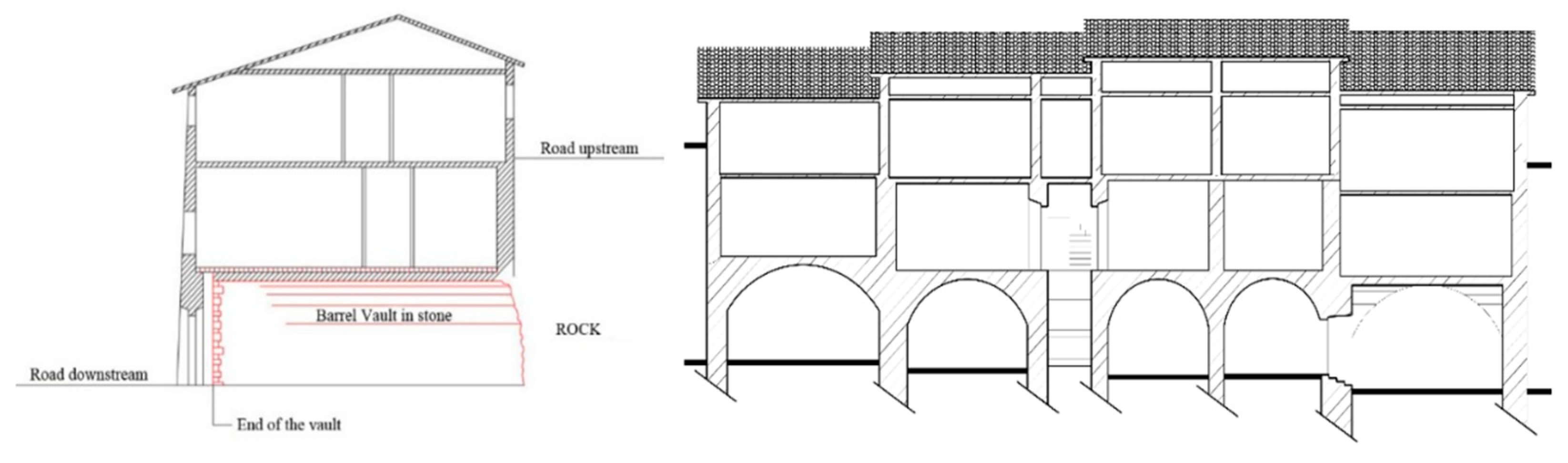
4.1. General Features and Structural Aggregates (SAs)

The building heritage of Campi Alto di Norcia covers an area of approximately 3.5 ha with 32 masonry aggregates (SAs) resulting in a total of 75 structural units (SUs), including three churches (i.e., Madonna della Piazza, Sant’Andrea and Santa Maria delle Grazie), fully destroyed by the 2016 earthquake sequence (Figure 2). According to the site morphology, SAs develop on three different levels, perpendicular to the slope of the hill on which the settlement is located. The first level has the entrance in correspondence of the downstream road and the top floor at the level of the upstream road.

The different levels and SAs are then connected through an internal organized system of staircases. The construction heritage of Campi Alto di Norcia is made up of both isolated masonry buildings and SAs arranged in rows, following the topography of the land. The gross building total volume and area are respectively about 15,000 m³ and 3065 m².

The SAs differ in terms of number, shape and height of SUs constituting them. In volume, isolated buildings cover the 29% of the whole stock (resulting in a volume of about 4243 m³), while external (end position) and internal (in between) SUs cover, respectively, the 44% and 27% of whole constructions (i.e., 6577 and 4035 m³). The number and height of the floors, the maintenance conditions and the materials adopted (both for vertical and horizontal structures) are different for each structural unit.

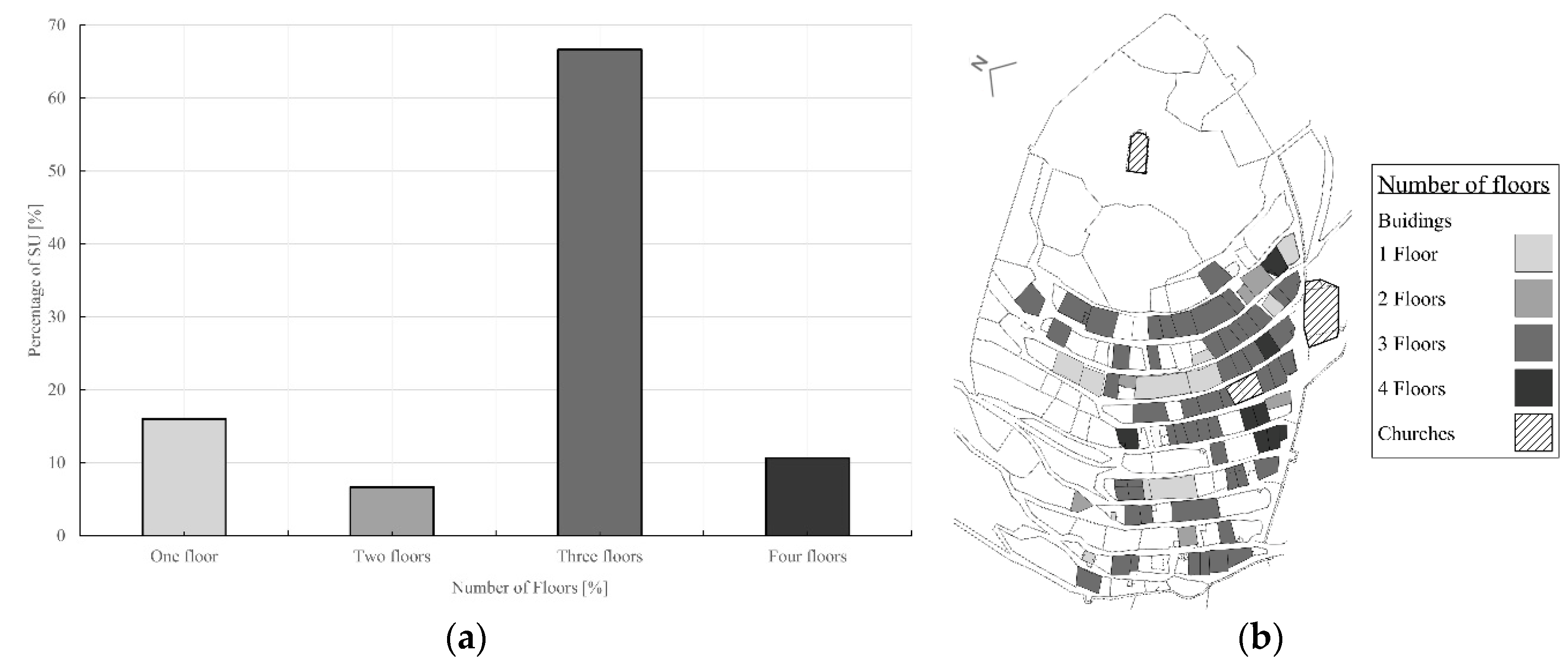
4.2. Structural Units: Main Features and Classification

The typical SU is organized on three storeys: the ground floor–partially underground following the hill’s slope–and two additional upper floors. A barrel masonry vault carved into the rock is usually present at the ground level, while the storeys of the other floors, as well as the roof, show the typical wooden structure sometimes replaced by reinforced concrete elements, such as concrete slabs or ring beams, in case of retrofit interventions over the years (Figure 3).

The average inter-storey height of the single SU is about 3.0 m. Masonry walls show different thickness along the height, with average values around 120 cm at the ground floor and reductions up to 70 cm in the upper levels. About the 16% of the buildings surveyed are one-storey constructions, often representing the rest of medieval houses.

Two, three and four-storey buildings represent respectively about 7%, 66% and 11% of the whole constructions (Figure 4). Normally, the organization of the SUs is the same, with a barrel vault at the first level and wooden or concrete slabs in the upper ones.

Two main categories of horizontal storey typologies can be recognized, i.e., rigid and semi-rigid (or deformable) ones, in relation to the presence (or the lack) of concrete slabs and crossed/single timber joints. Steel ties and concrete rings to connect timber floors to walls and/or masonry opposite walls are frequently introduced (Figure 5a), providing the difference between “bad” and “good” connection to the vertical bearing system: the presence of these elements and their workmanship define a “good” connection, while the absence or bad quality of the anchors identify a “bad” connection. Concerning the roof system, buildings in Campi Alto di Norcia have typically a mono-pitched or gable roof structure, being about 80% realized with steel/concrete beams and concrete slabs, avoiding horizontal thrusts acting on the external walls; the remaining 20% shows wooden structures, completed by a roof overhang placed on the perimeter of the aggregate. The roof typologies are therefore divided in “Heavy” or “Light” if made of concrete/steel or wood, and in “Thrust” or “No Thrust” when they span perpendicular or parallel to the main façade (Figure 5b).

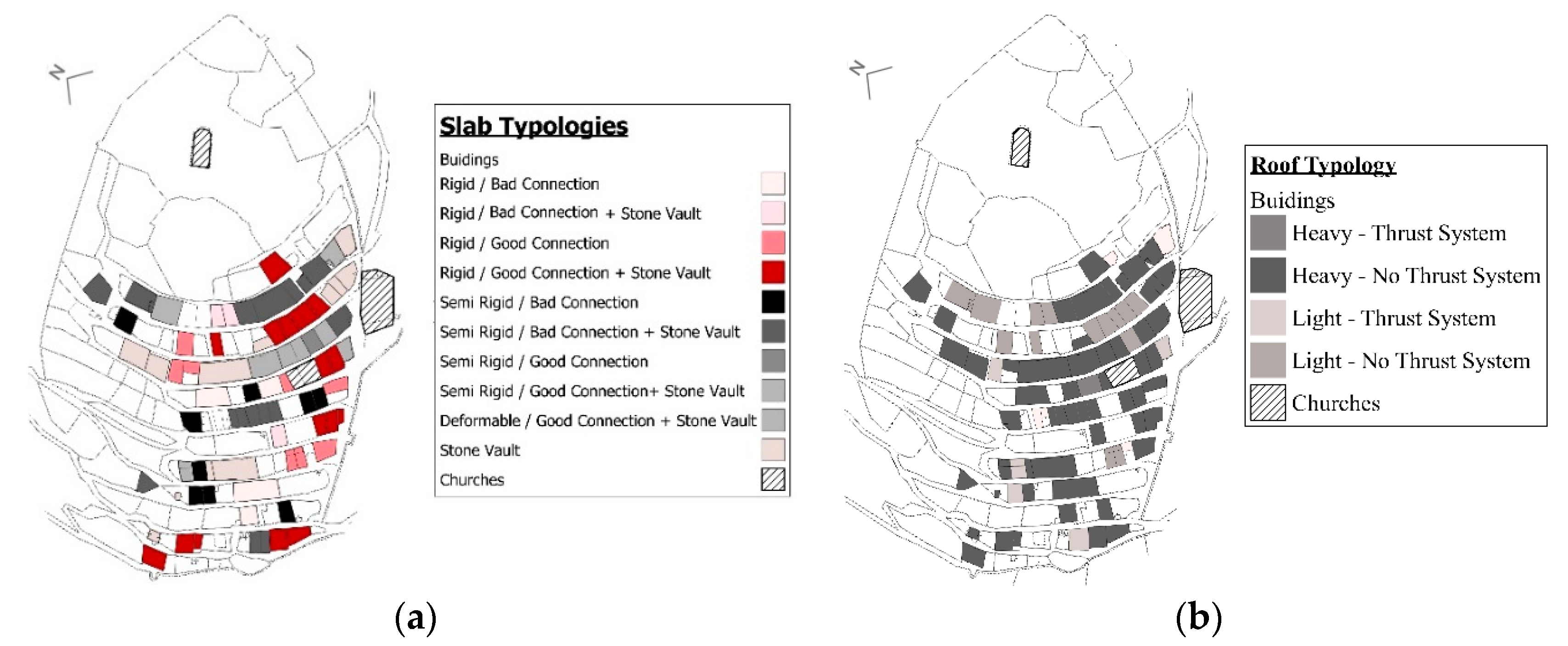
4.2.1. Materials and Masonry Typologies

The classification of the masonry typologies of the SUs is performed looking at their conservation condition (i.e., presence of deterioration phenomena, cracking patterns, etc.) and at the disposition of resistant blocks; of course, if needed, to the specific masonry typology can be then associated a conventional strength (i.e., mechanical properties) basing on indications provided by current standards and/or scientific literature database. Four different masonry typologies, all belonging to the general irregular masonry typology, have been recognized; only in a few cases, e.g., in the presence of new SUs or in retrofitted portions, the inner face of the walls is composed by regular brick blocks, while the external face consists of irregular masonry. More details are provided in

Table 3. Masonry typologies identified in the different SUs of Campi Alto di Norcia.

Masonry Typology		Description
		Irregular masonry typology with old and new (mixed) blocks Rough-hewn limestone units; this category includes other sub-categories, with differences related to the amount of mortar used for the walls. These masonry typologies have been detected in SUs where the original masonry was merged with a new one.
		Irregular masonry typology with no evident courses and thick mortar layer Masonry walls made of uncut limestone blocks, i.e., with no evident courses. This type of masonry represents the majority of masonry in Campi Alto di Norcia, where the wall is composed of two weakly-connected leaves. Typically, the outer face is not plastered and presents an irregularly arranged masonry, whereas the inner one is plastered.
		Irregular masonry type with irregular packed blocks Mixed structures made of both rough and squared limestone blocks. This is different from the previous one because of less mortar amount is present in the masonry. Again, this type of masonry, together with the previous one, is widely diffused in Campi Alto di Norcia.
		Regular masonry typology Squared bricks with regular courses: established entirely from squared ashlars, laid with a thin lime bed. These masonry types have been detected in new SUs or in portions of new masonry.

.

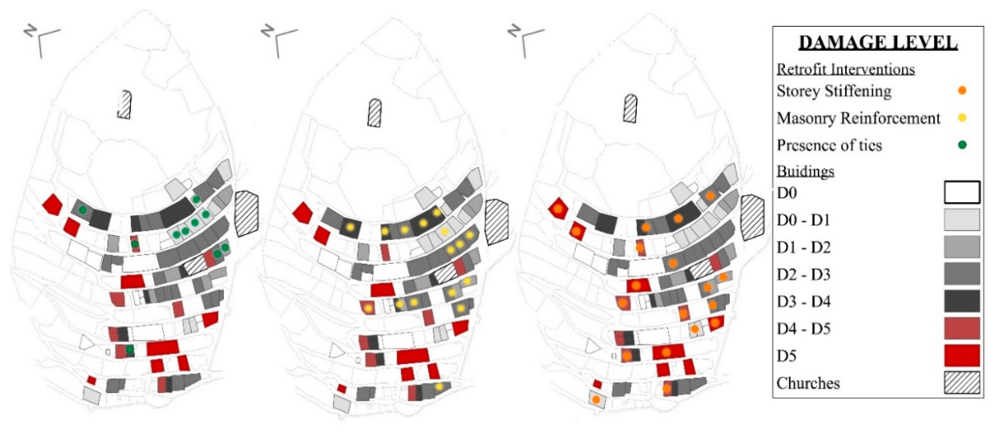
4.2.2. Retrofitting Systems

The historical development of masonry aggregates, which leads to superposition of several structural elements, strongly influences their seismic vulnerability evaluation. The reliability of empirical methods, which need to standardize the assessment methodology, decreases and this aspect is even more relevant if poor information about the buildings is available. For example, by comparing the year when the building was retrofitted with the technical standards of that time, it is possible to have an idea of the restoration techniques employed and, therefore, of the possible related vulnerabilities. An investigation of the construction year of the buildings and of the eventual application of retrofitting technique was performed, after gathering and analysing original documentation and drawings. In general, masonry buildings constituting SAs were realized before 1900, with the exception of SU1019, built after 2000, and SUs 95, 96, 120, 170 and 173, reconstructed in the 1980s (Figure 2b).

Retrofit operations detected in Campi Alto di Norcia can be divided into two main categories in relation to their execution, i.e., before or after the Valnerina earthquake of the 1979 (old/modern retrofit). The most common operations, in the first case, were the addition of masonry buttress to the external wall of the SU, the introduction of metal ties to connect the opposite wall facades of the buildings, etc. Modern retrofit—performed even after the 1997 Umbria–Marche seismic event—consisted in the replacement of timber roofs and timber floors with concrete slabs, in the application of injections and steel stitching to fill the voids in the masonry walls and to connect different masonry faces. Concrete plates to connect the walls with the new floors and roofs are also common, as well as reinforced cement-based plaster to reduce the irregularity of the masonry composition.

As a general remark, the fragilities detected in buildings are caused by the inconsistencies between the reconstructed and preserved parts, as well as the inadequate connections between the new and the original masonry. An example is the cement-based plaster employed for the reconstruction of the upper floors, just added for aesthetic reasons. Similarly, the demolition and reconstruction of vertical and horizontal structural elements with modern materials at the ground floor level result in local vulnerabilities [6].

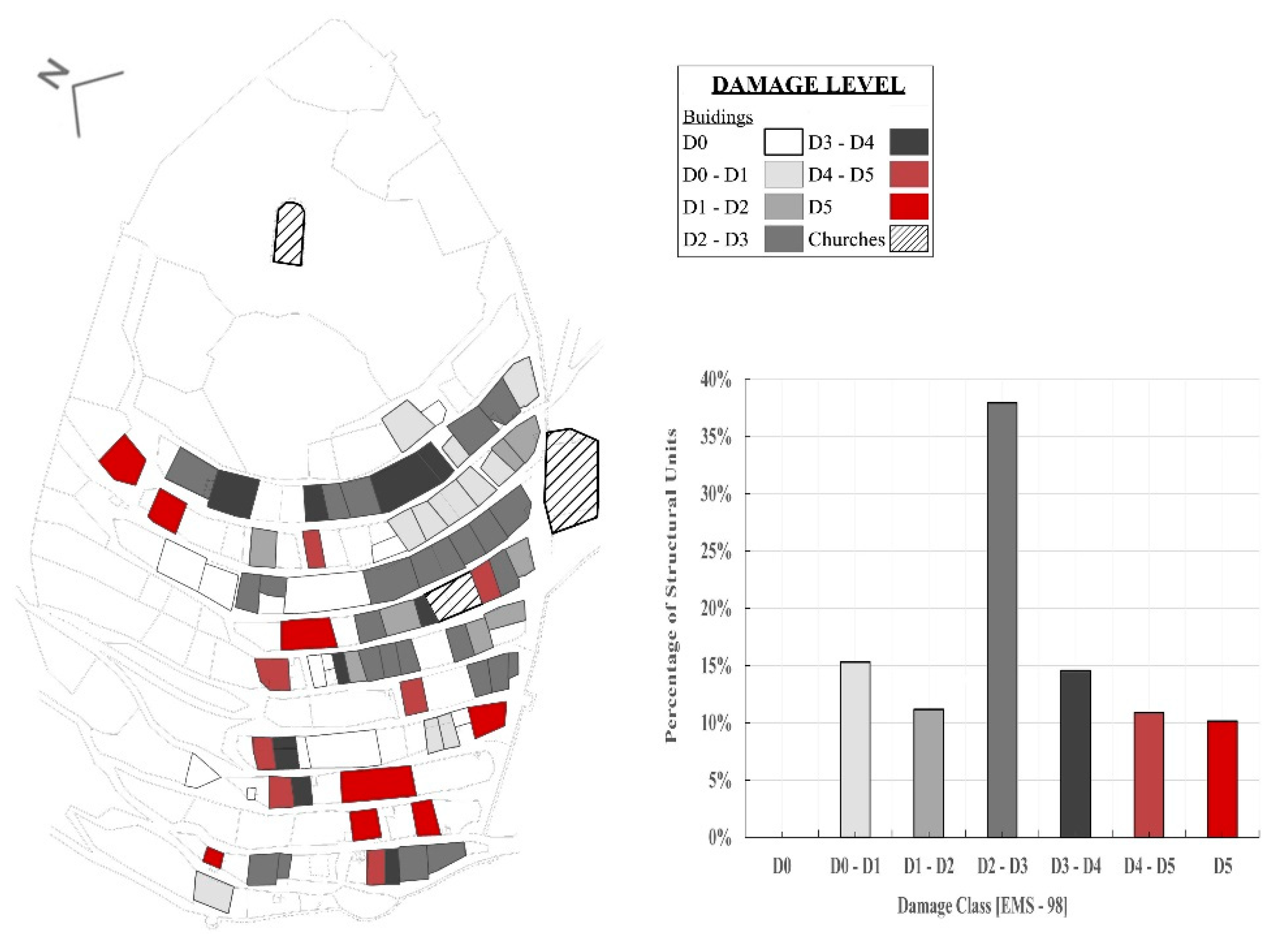
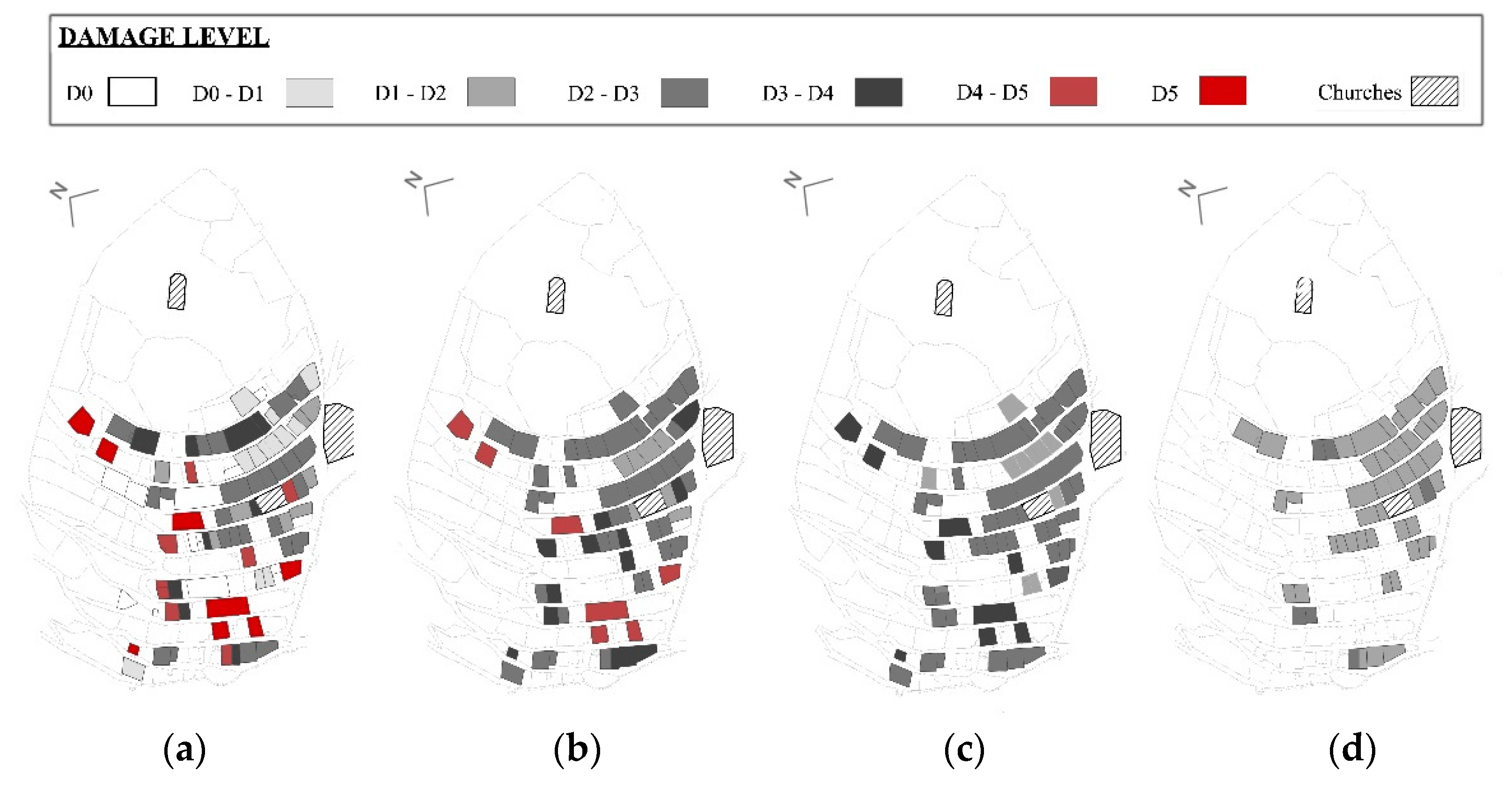
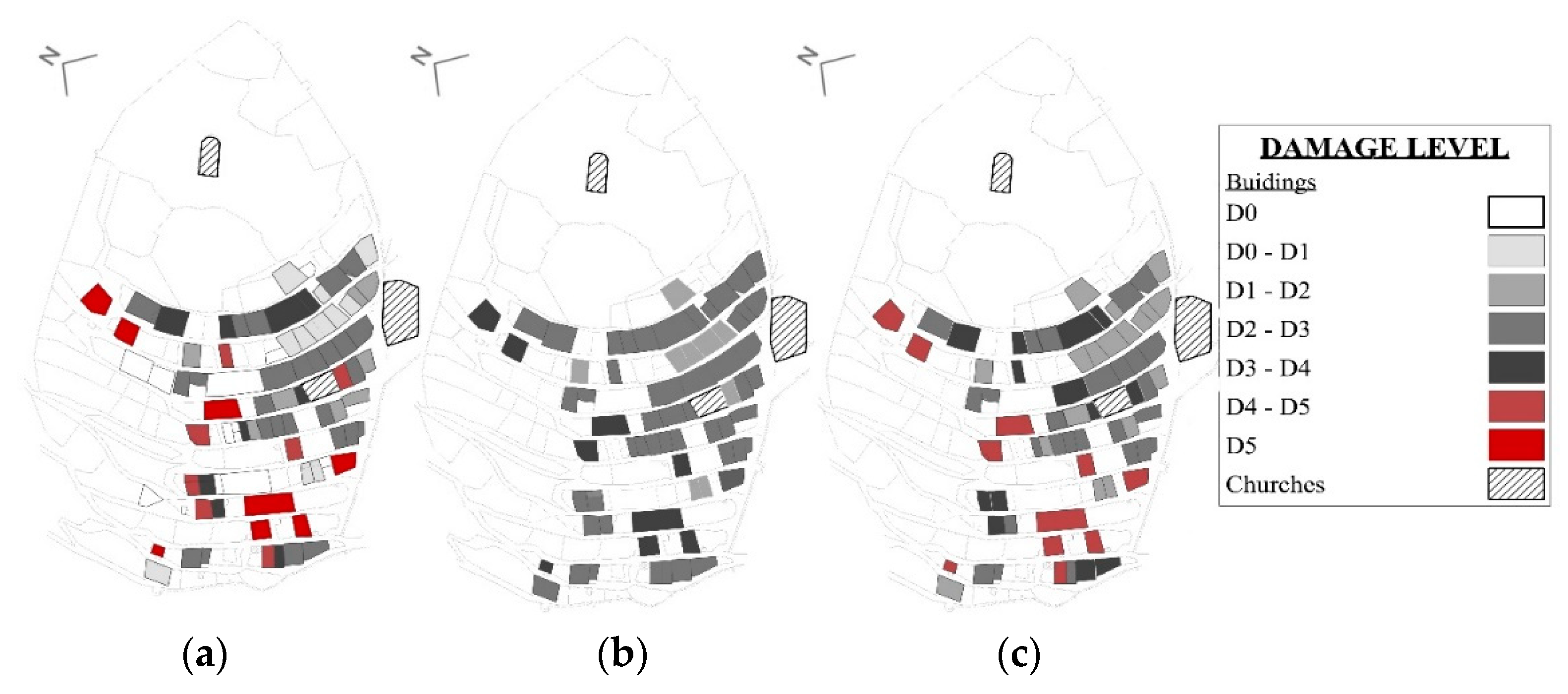
4.3. Damage Survey and Assessment through EMS98 Procedure

The seismic event of August and October 2016 required the deep in-situ surveys of the structural damages undergone by the buildings constituting the historical city centre of Campi Alto di Norcia. Inspections were performed in the immediate post-emergency phase, by expert technicians following the indications of the AEDES forms [28] for the detection of the partial and local collapses, cracking scenarios, structural failures, resulting deficiencies, etc. The European Macroseismic Scale (EMS)98 [29] was then adopted and applied to the different constructions with the aim of assigning a ‘damage class’ to each SU of Campi Alto di Norcia. The EMS98 scale provides graphical illustrations and descriptions of six different increasing damage levels—DL (i.e., D0, D1, D2, D3, D4 and D5—corresponding, respectively, to the lack of damage, negligible to slight, moderate, substantial to heavy and very heavy damage, and full destruction). With the aim of reducing the variability related to the personal expertise of the surveyor [28], three different independent judgements were used, applying then the average to the performed estimations.

Table 4. Damage distribution organized according to the volume and the number of buildings involved.

Damage Level (DL) and General Description		N° of SUs	% SUs	m3	%
D0	No damages	0	0%	0	0%
D0–D1	No structural damage and slight non-structural damage	11	16%	2120	15%
D1–D2	No structural damage and roof tiles detachment	9	13%	1550	11%
D2–D3	Slight structural damage and partial collapse of chimney and roof tiles’ detachment	25	39%	5260	38%
D3–D4	Large and extensive cracks in most walls and chimney fracture at the roofline	9	13%	2030	15%
D4–D5	Partial structure failure of roof and floors	6	9%	1510	11%
D5	Total collapse of the building	7	10%	1400	10%
	Total	67	100%	13870	100%

and Figure 6 show the distribution of the damage level for SUs, in terms of percentage of buildings and volume of construction. Most SUs shows a DL equal to D2–D3 and D4–D5, but most of the volume turns out to be in the range D2–D3, since many SUs, used as storage areas and cellars with a low volume, are nowadays fully collapsed. Storage areas and cellars were not further considered in the assessment procedure, therefore reducing the number of analysed SUs to (only) 67.

Figure 7 shows a comparison performed, in a GIS environment, between the DL of the SUs and the retrofit interventions carried out after the seismic events of 1979 and 1997. Most of the SUs, where the timber roofs and timber floors were replaced with concrete slabs (“storey stiffening” intervention marked in red), show a damage level D4–D5. The SUs reinforced with injections and steel stitching (“masonry reinforcement” marked in yellow) have an average DL around D3, while the SUs with the lowest DL are the ones characterized by the presence of ties on the façade (marked in green).

5. Seismic Vulnerability Assessment of Campi Alto di Norcia

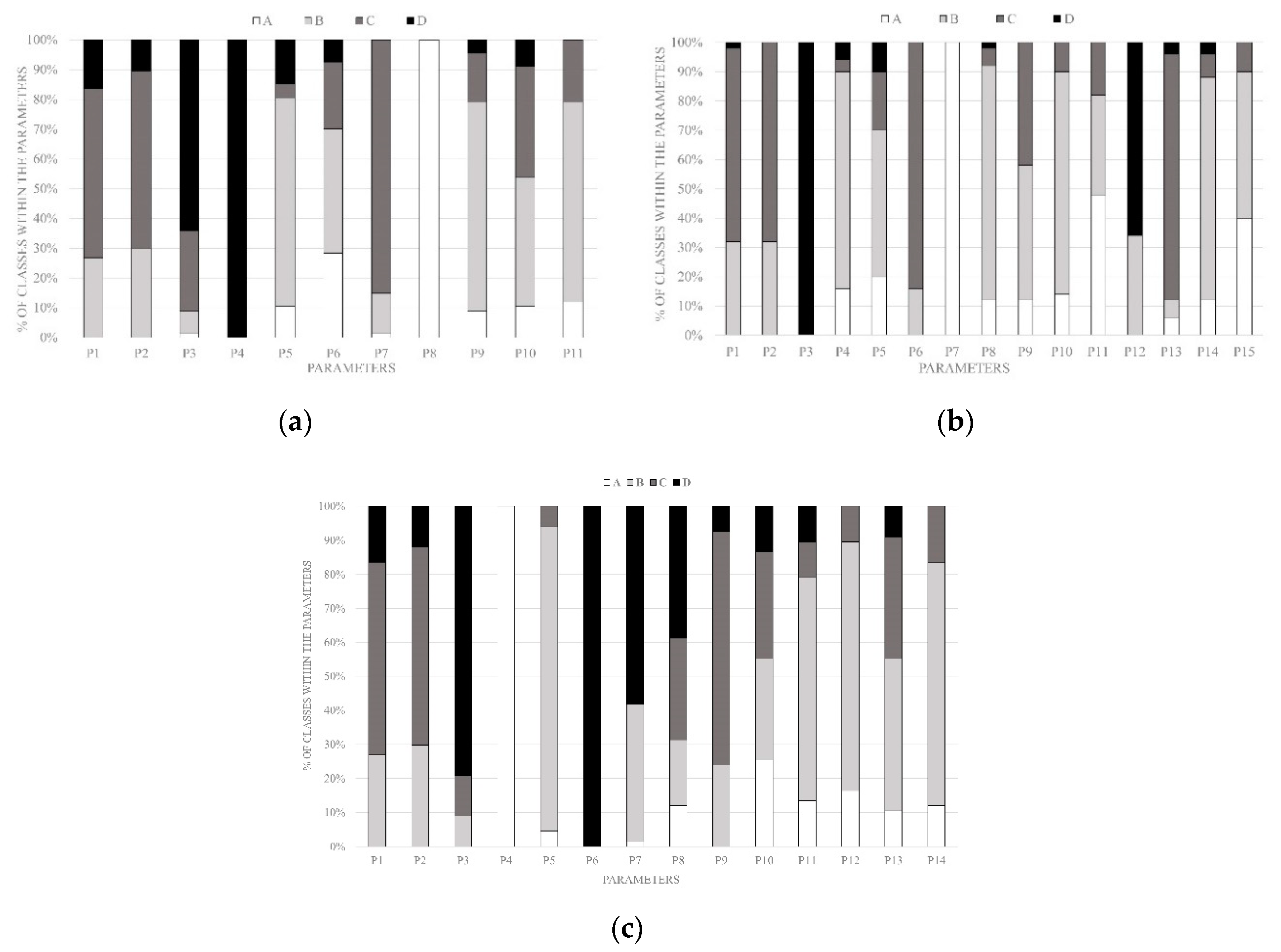
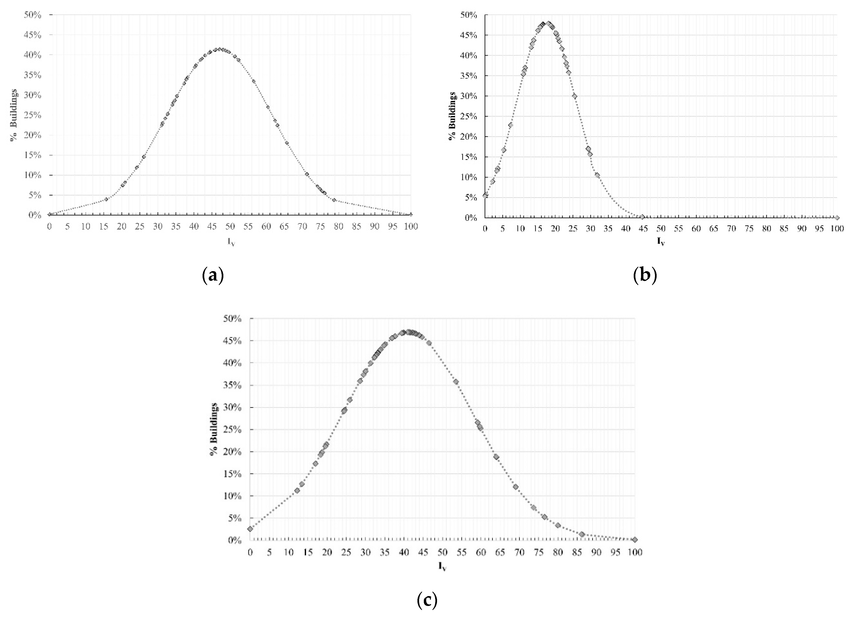
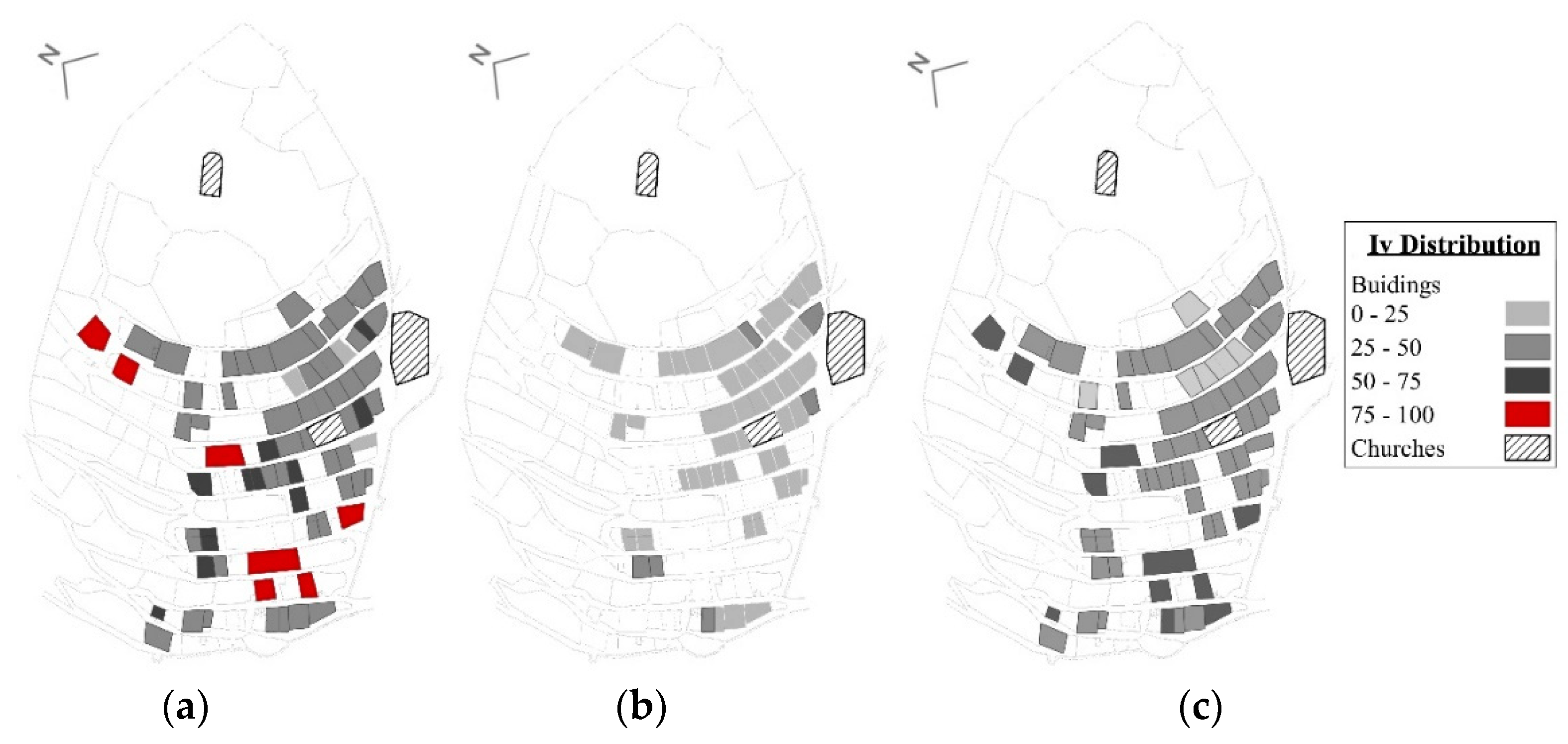
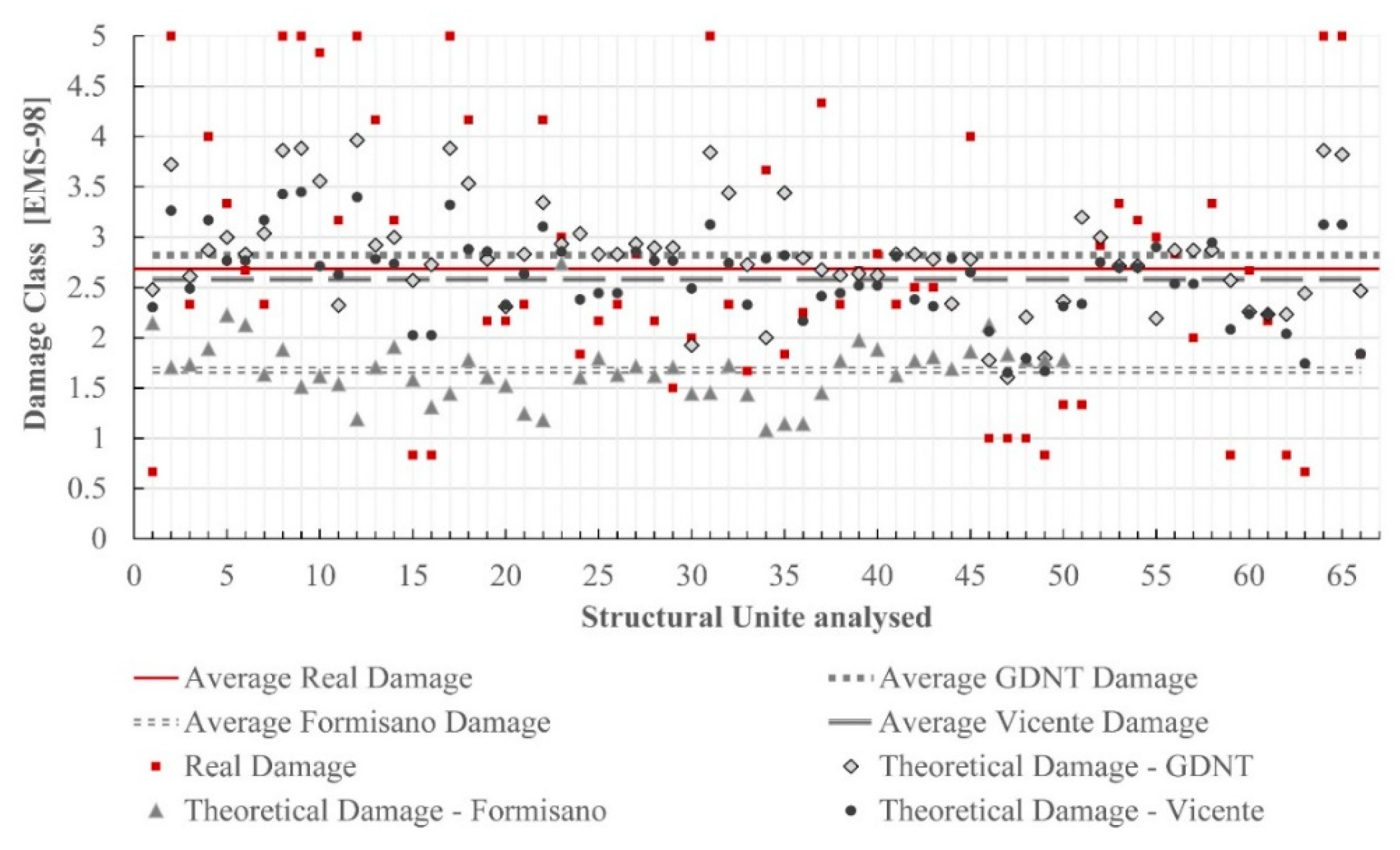
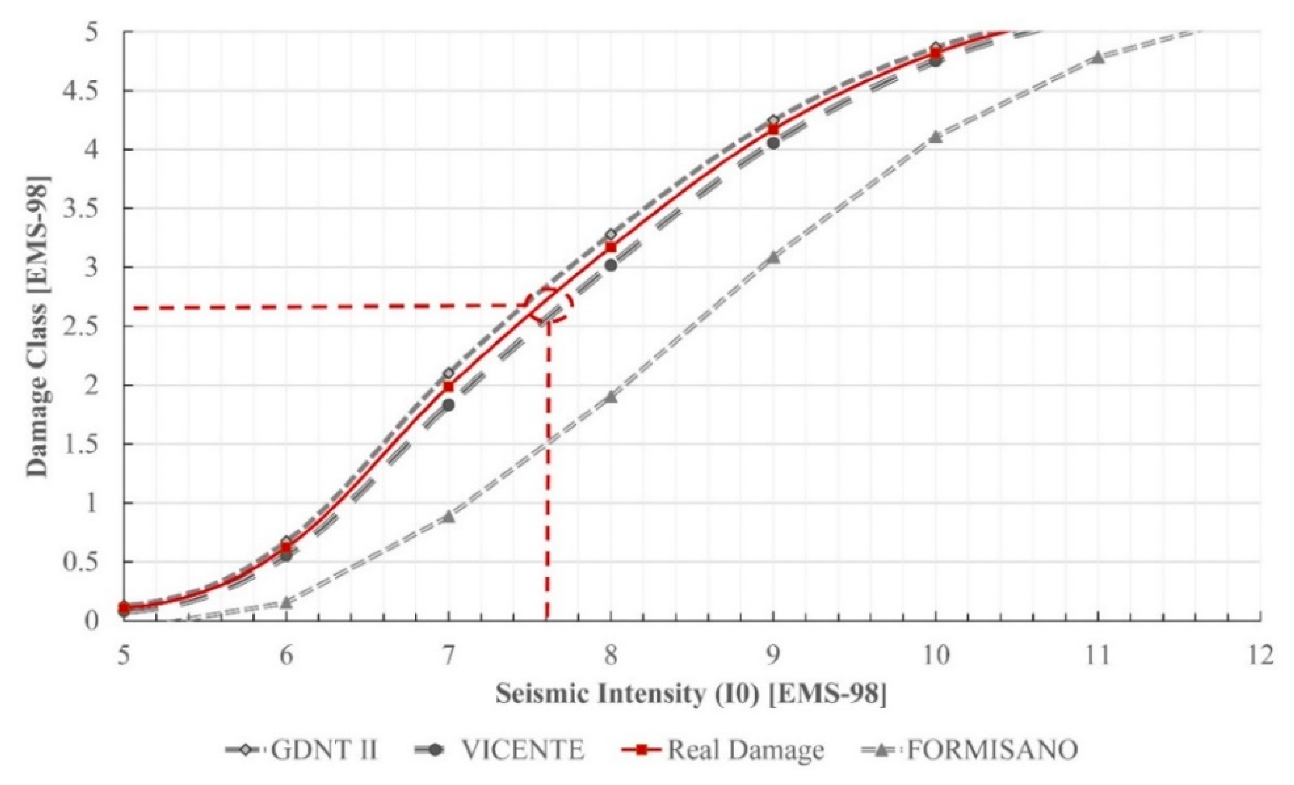
5.1. Application of Traditional Vulnerability Index (I_V) Methodologies and Results

The statistical approach used for the seismic vulnerability assessment of masonry buildings at urban scale is the vulnerability index method (I_V method), originally developed by [30] and later revisited by [31,32,33]. The method is based on defining the seismic vulnerability of an SU within an SA through the analysis of several parameters—selected in relation to the structural typology—provided by a “weight” and finally defining a vulnerability index (1). Resulting values are usually normalized in the range 0 ÷ 100 [34] (2). The I_V evaluation is performed based on a comprehensive survey of the building, where the relevance of each parameter, measured by its weight, is defined based on post-earthquake damage observation. Having determined the hazard level of the territory resorting to an intensity scale, it is possible to evaluate the expected damage scenarios of a specific area using semi-empirical methods [35].

$${\mathrm{I}}_{\mathrm{V}}^{*}=\sum {\mathrm{p}}_{\mathrm{i}}·{\mathrm{c}}_{\mathrm{i}}\mathrm{where}\{\begin{array}{c}{\mathrm{c}}_{\mathrm{i}}=\mathrm{vulnerability} \mathrm{class} “\mathrm{i}”\\ {\mathrm{p}}_{\mathrm{i}}=\mathrm{weight} \mathrm{i}\end{array}$$

(1)

$${\mathrm{I}}_{\mathrm{V}}={\mathrm{I}}_{\mathrm{V}}^{*}\mathrm{normalized}\mathrm{to}100\%$$

(2)

Current vulnerability index methodologies were developed and calibrated basing on specific constructions’ typologies, being then provided by good reliability for buildings belonging to those categories but decreasing their if relevant differences are present. In the present research work, three traditional approaches were used: the GNTD method [21], the Formisano method [22] and the Vicente approach [35], being more appropriate for the considered context.

The GDNT method [21] adopts for the I_V evaluation eleven parameters (namely P1 to P11) and four vulnerability classes (A to D, being A the best condition and D the worst one); the method was developed for isolated buildings, taking into account their geometry, structural and non-structural features, the floors and roof typologies, walls thickness and maintenance conditions. The maximum value of the achievable non-normalized I^*_V is equal to 382.5.

With the aim of improving the [21] procedure by considering the SA effect and the interaction among SUs, Formisano [22] introduced five additional parameters: the position of the SU in the aggregate, the percentage of openings in the façade walls, the presence of staggered slabs, the structural difference between adjoining SUs and the interaction of neighbouring SUs with different heights. Compared to the GDNT method, this approach disregarded, at least in an explicit manner, the qualitative resistance of the walls. Some of the weights were also redefined. Negative values were assigned with the aim of reducing the vulnerability. The maximum value of the achievable non-normalized I^*_V is equal to 515.25.

The Vicente method [35] introduced 4 macro-classes of parameters related to the structural building system (P1 to P4), to the irregularities and interaction (P7 to P10), to floor slabs and roof (P11 to P12), to conservation status and other elements (P13 to P14); 3 new parameters (P4, P6 and P7) were also introduced. The maximum value of the achievable non-normalized I^*_V is equal to 650.

Table 5. Summary table of vulnerability parameters adopted by the different methods.

Vulnerability Parameters			Short Description	Vulnerability Class				Weight
				A	B	C	D
GNDT (1994)	P1	Organization of vertical structures	Age of the construction and connection typology between the walls	0	5	20	45	1
	P2	Nature of vertical structures	Vertical element typology	0	5	25	45	0.25
	P3	Qualitative resistance	Walls’ shear strength assuming box behaviour	0	5	25	45	1.5
	P4	Location of building and type of foundation	Slope and quality of the foundation soil	0	5	25	45	0.75
	P5	Floor typology	Quality of floor type considering stiffness and connection with the walls	0	5	15	45	1
	P6	Plan regularity	Length/width ratio of the building plan	0	5	25	45	0.5
	P7	Height regularity	Mass variation in elevation and the presence of arcades or towers	0	5	25	45	1
	P8	Distribution of plan resisting elements	Spacing between walls	0	5	25	45	0.25
	P9	Roof typology	Weight and characteristics (thrust) of the roof	0	15	25	45	1
	P10	Non-structural elements	Presence, typology and connection to the building	0	0	25	45	0.25
	P11	Physical conditions	Masonry quality and cracking scenario	0	5	25	45	1
Formisano (2014)	P1	Organization of vertical structures	Age of the construction and connection typology between the walls	0	5	20	45	1
	P2	Nature of vertical structures	Vertical element typology	0	5	25	45	0.25
	P3	Location of building and type of foundation	Slope and quality of the foundation soil	0	5	25	45	0.75
	P4	Floor typology	Quality of floor type considering stiffness and connection with the walls	0	5	15	45	0.75
	P5	Plan regularity	Length/width ratio of the building plan	0	5	25	45	0.5
	P6	Height regularity	Mass variation in elevation and the presence of arcades or towers	0	5	25	45	1
	P7	Distribution of plan resisting elements	Spacing between walls	0	5	25	45	1.5
	P8	Roof typology	Weight and characteristics (thrust) of the roof	0	15	25	45	0.75
	P9	Non-structural elements	Presence, typology and connection to the building	0	0	25	45	0.25
	P10	Physical conditions	Masonry quality and cracking scenario	0	5	25	45	1
	P11	Misalignment of openings SU	% difference of openings in adjacent facades	−20	0	25	45	1
	P12	Masonry disconnections	Effect of structural or typological heterogeneity in adjacent SUs	−15	−10	0	45	1.2
	P1	Presence of adjacent buildings with different height	Location of the SU in the SA and height’s variation	−20	0	15	45	1
	P14	Position of the SU in the SA	Number of sides next to other SUs	−45	−25	−15	0	1.5
	P15	Presence and n° of staggered floors	Number of staggered floors in the SA	0	15	25	45	0.5
Vicente (2010)	P1	Type of resisting system	Construction age, quality of walls’ connection	0	5	20	50	0.75
	P2	Quality of the resisting system	Vertical Element Typology	0	5	20	50	1
	P3	Conventional strength	Walls’ shear strength assuming box behaviour	0	5	20	50	1.5
	P4	Maximum distance between walls	Spacing between walls	0	5	20	50	0.5
	P5	Number of floors	Number of floors in the building	0	5	20	50	1.5
	P6	Location of building and type of foundation	Slope and quality of the foundation soil	0	5	20	50	0.75
	P7	Aggregate position and interaction	Position of the SU in the SA	0	5	20	50	1.5
	P8	Plan configuration	Length/ width ratio of the building plan	0	5	20	50	0.75
	P9	Height regularity	Mass variation in elevation and the presence of arcades or towers	0	5	20	50	0.75
	P10	Wall façade openings and alignments	Influence of the misalignment	0	5	20	50	0.5
	P11	Horizontal diaphragms	Quality of floor type considering stiffness and connection with the walls	0	5	20	50	1
	P12	Roof typology	Weight and the roof typology (thrust)	0	5	20	50	1
	P13	Fragilities and conservation state	Masonry quality and cracking scenario	0	5	20	50	1
	P14	Non-structural elements	Type and characteristics of the non-structural elements	0	5	20	50	0.5

summarizes the parameters adopted in the different methods, vulnerability classes and weights associated. As visible, the three approaches have several common parameters even if the weight associated can slightly vary.

Figure 8 shows the vulnerability classes and the influence that every single parameter has in the overall seismic vulnerability assessment, considering the three different methods. The topography of settlement (P4 for GDNT, P3 for Formisano and P6 for Vicente) strongly penalizes the seismic vulnerability of the buildings, resulting in class D.

On the contrary, the small size of the buildings and the low spacing between walls have a positive impact on their vulnerability (P8 for GDNT, P7 for Formisano and P4 for Vicente), although relatively limited on the final I_V.

The application of the GNDT method to Campi Alto di Norcia results in an average I_V equal to 47 with standard deviation (SD) of 14 (Figure 9). The values of the normalized I_V—evaluated according to [2]—are between 20 and 30 for the 6% of the SUs analysed and between 30 and 40 for the 19% of the SUs. The remaining 43% shows I_V within the range 40–50, 9% in the range 50–60, 7% in the range 60–70 and, finally, 12% in the range 70–80. The remaining SUs present a seismic vulnerability index value lower than 20. The Formisano method [22] was used to account for aggregate effects within SUs: isolated buildings were then neglected, leading to the analysis of only 50 SUs. The achieved normalized I_V values [2] are between 0 and 10 for 13% of the SUs analysed and between 10 and 20, 20 and 30, respectively, for 44% and 35% of SUs. The remaining buildings show a seismic vulnerability equally distributed in the ranges 30–40% and 40–50%. As a general remark, the Formisano method [22] provides a lower vulnerability of SAs of Campi Alto di Norcia, with an average I_V value of 17 and a standard deviation (SD) equal to 9 (Figure 9). For the sake of comparison, considering the same 50 SUs, the GNDT indicates an average normalized I_V value of 43 and an SD of 10. Finally, the adoption of the Vicente method (2010) led to an average normalized I_V equal to 41 and a standard deviation (SD) of 11; in terms of distribution, 4% of the evaluated buildings shows an I_V index between 10 and 20, 12% between 20 and 30, 30% between 30 and 40, and, finally, the remaining 35% between 40 and 50 (Figure 9). Again, for the sake of completeness, considering only the 50 SUs in SAs used in the Formisano method, the average I_V value is 39 with an SD of 9. Figure 10 summarizes the I_V distribution in the case study of Campi Alto di Norcia.

Trying to summarize the achieved results in terms of normalized values, the GDNT procedure is the method providing the highest I_V, possible consequence of ignoring of the aggregate effect’s influence. Regarding the trend of the data, the Formisano approach is the one that focuses results around the average value; the Vicente method, considering different vulnerability indexes for multiple buildings, shows the highest SD.

The results well reflect the influence of the weights and the vulnerability scores in the seismic vulnerability assessment, e.g., the low vulnerability values obtained from the Formisano approach are caused by parameters P4 (position of the building in the masonry aggregate) and P1 (percentage of opening areas among adjacent facades) owning a positive effect on the vulnerability results. Similarly, parameter P7 (aggregate position and interaction) of the Vicente method decreases the seismic performance of the SUs located at the corners, improving otherwise significantly the behaviour of the SUs inside the SAs. Figure 11 shows the distribution of the Iv in the case study, assessed with the different methods. What is presented above, in a general way, indicates relevant differences in the adoption of different methods that were, as said, calibrated basing on different case studies.

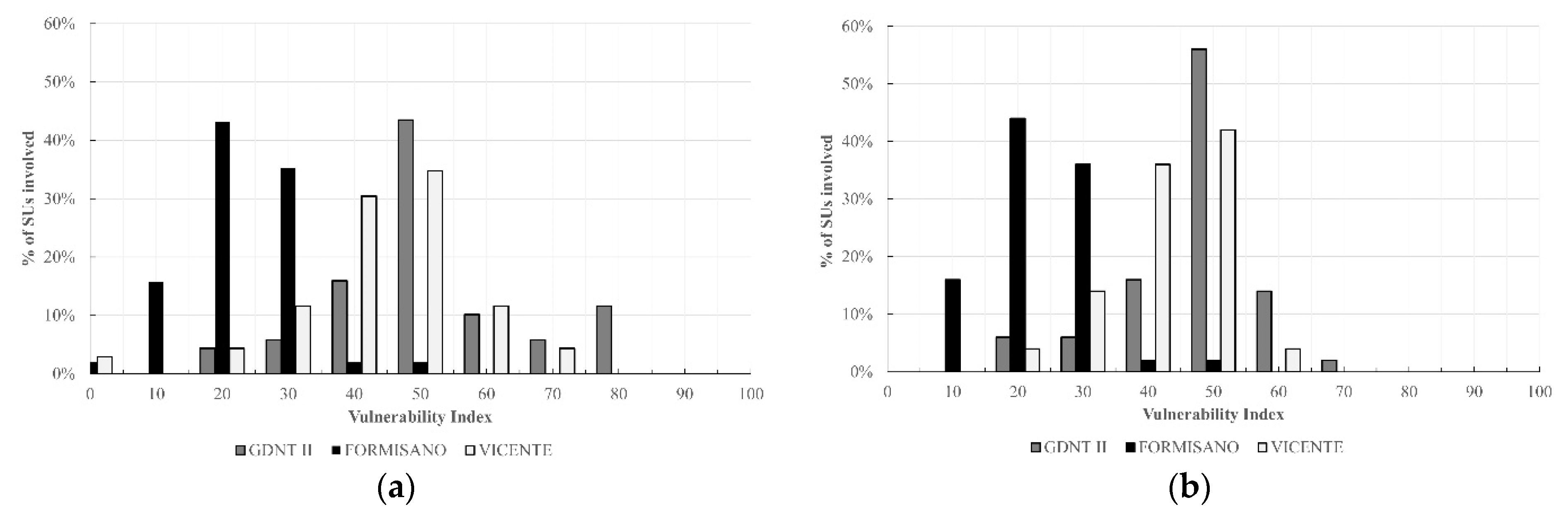
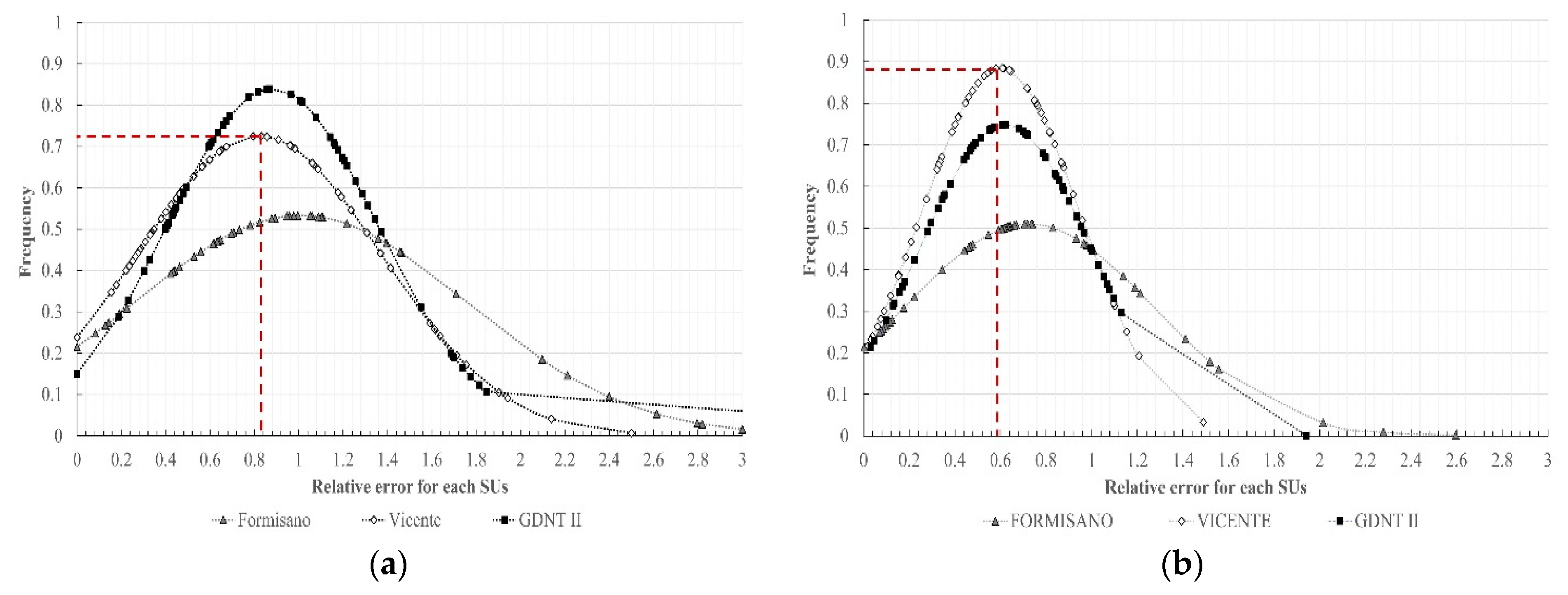
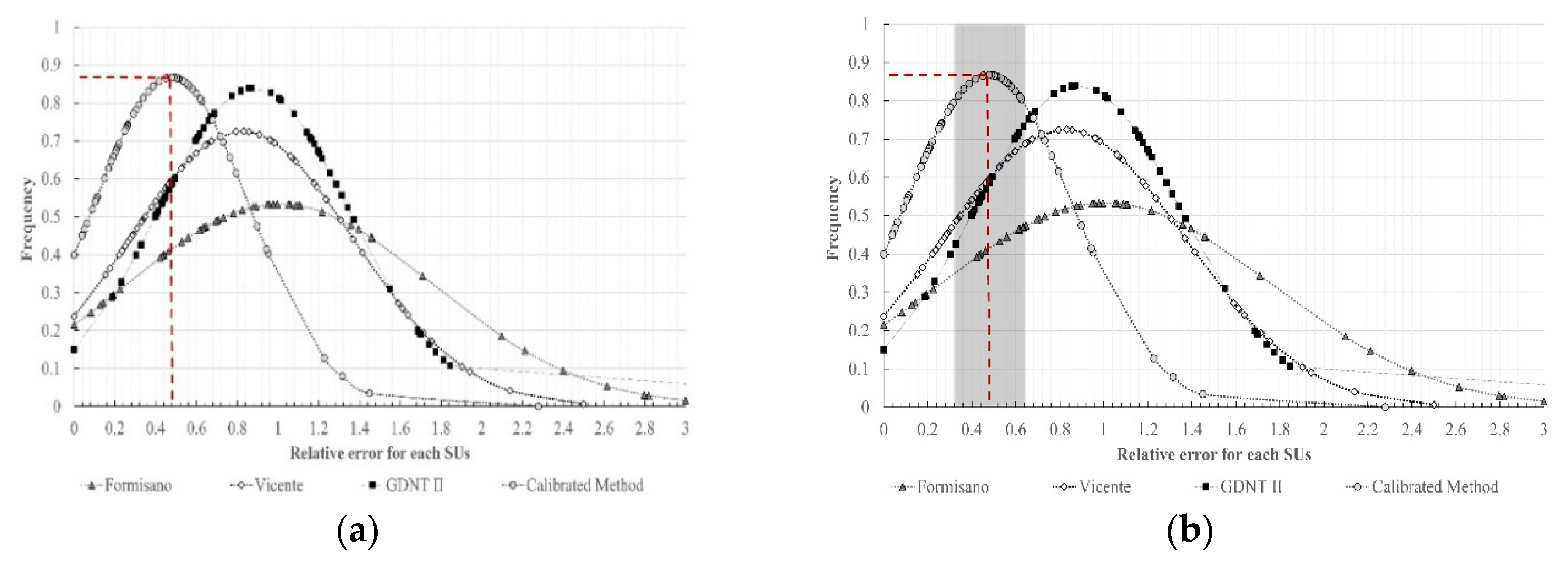
5.2. Reliability of the Seismic Vulnerability Methods

The reliability of the selected statistical methods for the buildings’ typologies of Campi Alto di Norcia was assessed by comparing the real damage data recorded after the 2016 earthquake sequence with theoretical damage scenarios evaluated through the above-presented I_V methods. For the evaluation of the theoretical damage connected to the different approaches, the formulation proposed by [31] was adopted:

$${\mathsf{\mu }}_{\mathrm{T}}=2.5+3·\tan \mathrm{h}\left(\frac{\mathrm{I}+6.25·\mathrm{V}-12.7}{\mathrm{Q}}\right)·\mathrm{f}\left(\mathrm{V},\mathrm{I}\right)$$

(3)

$$\mathrm{f}\left(\mathrm{V},\mathrm{I}\right)=\{\begin{array}{c}{\mathrm{e}}^{\frac{\mathrm{V}}{2}·\left(\mathrm{I}-7\right)} \mathrm{I}\le 7\\ 1 \mathrm{I}>7\end{array}$$

(4)

$$\mathrm{V}=0.56+0.0064·{\mathrm{I}}_{\mathrm{V}}$$

(5)

being V the vulnerability calculated from the I_V value, I the intensity using the European Macroseismic Scale 1998 (EMS98) using numbers between I (not felt) and XII (complete destruction) for the individual classification of earthquakes, Q the ductility factor and μ_T the damage value in the EMS98 scale, varying between 1 (negligible to slight damage) and 5 (destruction) according to [29]. Based on post-seismic damage evaluations of irregular brick masonry buildings and on [36], a ductility factor of 2.5 was adopted for masonry buildings with sufficient ductile behaviour.

To measure the strength of shaking produced by the 2016 earthquake at Campi Alto di Norcia in October 2016, the magnitude, as well as the accelerograms, of the Campi Station (Table 2) were transformed into a macroseismic intensity; the results were then compared with data collected by the technician, who surveyed the damages just after the seismic events [37]. Finally, an intensity I_MCS equal to 8.5, evaluated with the MCS scale, was assigned to the case study [38]. Since the damage assessment was performed, as already said in the previous paragraph, through the European Macroseismic Intensity, to correlate the two intensity measures the analytical expression provided by [39] was used:

$${\mathrm{I}}_{\mathrm{EMS}98}=0.734+0.814·{\mathrm{I}}_{\mathrm{MCS}}=7.65\approx 8.0$$

(6)

The relative error was evaluated as the difference between the theoretical and the observed damage in the case study after the seismic events of October 2016, then related to that specific seismic event’s intensity (6).

The I_v method reliability was calculated as the mean relative error of the values achieved for the whole building stock analysed. The uncertainties affecting the methods are both epistemic and aleatory, being related to the features characterizing each aggregate, to the classification of buildings into a vulnerability class or construction typology [40].

To overcome these issues and to control with more accuracy the reliability of the I_V method, the vulnerability of each building was evaluated not as a single value but as a range referred to the whole historical city centre. By this way, the upper and lower bounds of the I_V were defined for each SU, considering the SD of the vulnerability assessment of Campi Alto di Norcia. This procedure allows obtaining, for each I_V, the possible vulnerability variation by taking into account the different assessments performed in the historic centre for the construction typology analysed. The aim was to evaluate a range of possible results for the seismic vulnerability of each building, whose amplitude is defined by the dispersion of the data with respect to the sample space. Resorting to Equation (3), it was then possible to achieve a reliable and credible range for the expected damage.

The accuracy of each statistical method was then evaluated as the minimum relative error achieved considering the theoretical damage scenario defined with the reduced I_V and with the increased I_V, compared to the real/observed one in the case study. A range of the initial level of expected damage was then established to perform the parametric analysis of the seismic vulnerability of the considered construction typology, evaluating the influence of the I_V methods in the seismic response of the buildings. The reliability of the I_V method was assessed, considering two typologies of relative error:

-

at the individual building level (${\overline{Err}}_{mean,d}$) considering the difference of the theoretical damage ($\overline{{\mu }_T})$, evaluated with the direct measure of the Iv of the single building, with the real damage observed $({\mu }_R^{})$;

-

at a global level (${\overline{Err}}_{mean,r}$), considering the difference of the theoretical damage scenarios defined with the reduced I_V $({\mu }_T^{-})$ and with the increased I_V $({\mu }_T^{+})$, with the real damage observed $({\mu }_R^{})$.

The comparison of the results achieved with the ${\overline{Err}}_{mean,r}$ and ${\overline{Err}}_{mean,d}$ provide import information about the possibility of evaluating the I_V of each building within a range, rather than for a single value. The next expressions (7) and (8) try to clarify the procedure adopted for each building:

$${\mathrm{I}}_{\mathrm{v}}=\{\begin{array}{l}{\mathrm{I}}_{\mathrm{v}}^{-}=\overline{{\mathrm{I}}_{\mathrm{v}}}-SD\to {\mu }_T^{-}\hspace{1em}\left(lowerbound\right)\to Er{r}_{-}=\left|{\mu }_R-{\mu }_T^{-}\right|\\ \overline{{\mathrm{I}}_{\mathrm{v}}}\to \overline{{\mu }_T}\hspace{1em}\hspace{1em}\hspace{1em}\left(directmeasure\right)\to Err=\left|{\mu }_R-\overline{{\mu }_T}\right|\\ {\mathrm{I}}_{\mathrm{v}}^{+}=\overline{{\mathrm{I}}_{\mathrm{v}}}+SD\to {\mu }_T^{+}\hspace{1em}\left(upperbound\right)\to Er{r}_{+}=\left|{\mu }_R-{\mu }_T^{+}\right|\end{array}$$

(7)

$$\begin{array}{c}{\overline{Err}}_{mean,d}=\left(\frac{\sum Err}{n}\right)\\ {\overline{Err}}_{mean,r}=\left(\frac{\sum \min \left({Err}_{-};{Err}_{+}\right)}{n}\right)\end{array}$$

(8)

Being Err the error for a given building defined as the difference between theoretical and real damage detected in the case study in absolute value, n the number of buildings, and $Er{r}_{-}$ and $Er{r}_{+}$ the errors in a given building as the minimum difference between theoretical damage, considering the upper and lower bounds, and the real one of the case study in absolute value.

Figure 12 summarizes the procedure adopted for the reliability evaluation of the selected I_V methods in the case study considering the vulnerability range for each building. The process was applied to each of the three I_V methods adopted, comparing the results obtained and assessing the lowest relative error (

Table 6. Evaluation of the Iv method reliability in the case study analysed.

	IV Method Accuracy (Direct Measure)		IV Method Accuracy (Assuming a Range)
IV Methods	Average relative errors	Variance relative errors	Average relative errors	Variance relative errors
GDNT II	0.87	0.67	0.67	0.37
Formisano	1.13	0.72	0.72	0.55
Vicente	0.85	0.61	0.58	0.34

).

As visible, none of the methods was able to estimate the observed damage of Campi Alto di Norcia with high accuracy, resulting in differences between real and theoretical damage, evaluated for each building, higher than 0.85 for all procedures (Figure 13). Considering a probable theoretical damage range, the relative errors decreased, remaining otherwise higher than 0.58. As already said, results highlight the poor accuracy of the methods if used under very different conditions than those assumed in their calibration processes.

To check if the relative error is caused by an overestimation or underestimation of the real damage by the different methods, the whole analysis of the damage distribution within the case study is necessary. Considering the mean value of the I_V range for each building in the SA, it is possible to compare results of the different methods at single building and urban scale levels. Figure 14 shows the comparison between theoretical and real damage distribution in Campi Alto di Norcia, carried out at building scale by evaluating, for each SU, the distance between the real and expected damage.

As visible, while real damage values are quite scattered, the distribution of the estimated damage is concentrated around the average values: this indicates the limits connected to the adoption of Equation (3) when estimating high or low damage classes for different vulnerability values.

Figure 15 shows otherwise the comparison between real and theoretical damage for Campi Alto di Norcia using the different vulnerability methods previously presented. Some preliminary conclusions can be drafted: the Formisano method [22] provides less conservative vulnerability values, with underestimation of the real damage; the average value of the real damage lies in the middle between the GDNT [21] and the Vicente [35] methods, showing how the latter can better catch the influence of the aggregate effect for the present case study.

What is herein presented concerns the comparison between real/theoretical damage for the different methodologies applied to the case study related to the specific seismic event of 2016 and, therefore, to its specific intensity. Extensions are otherwise needed to provide a general overview of the effective vulnerability of the case study.

By considering the average vulnerability values obtained for the different approaches and changing the macroseismic intensity, it is possible to numerically develop various damage scenarios for the urban centre of the case study analysed, following Equation (3). The vulnerability curves presented in Figure 16 show how these methods overestimate or underestimate the real damage even for different macroseismic intensities. The curve representing the real damage of the case study for different seismic intensity is a simple forecast, achieved through the average vulnerability value obtained from the real damage detected through Equation (3).

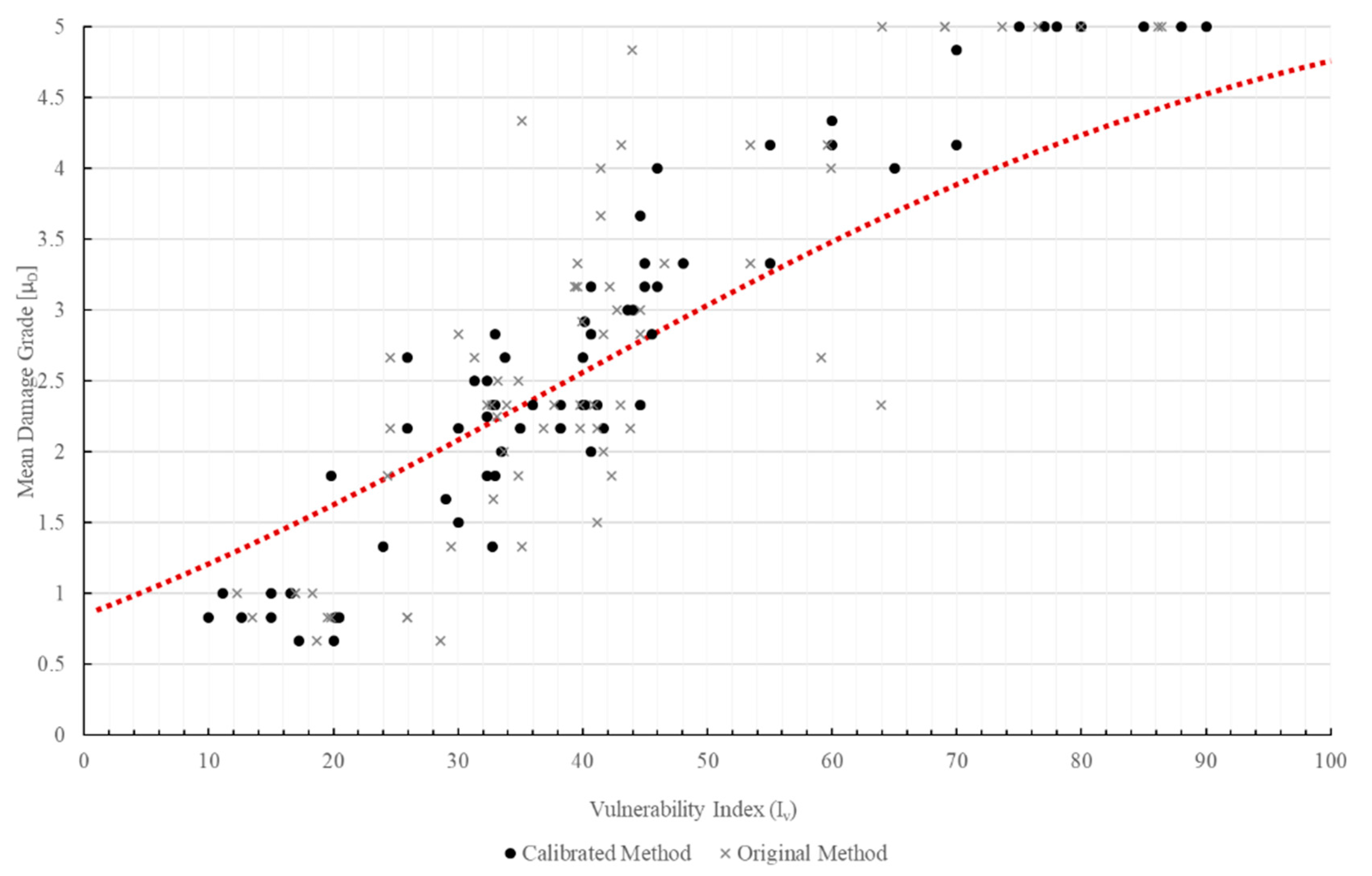
6. Calibration of the Vicente I_V Method for Campi Alto di Norcia

Stating the results previously presented, the Vicente method is the one showing more performing results and, besides, including aggregate considerations; with the aim of achieving an I_V method suitable for damage prediction in Campi Alto di Norcia, a calibration procedure was performed to opportunely modify the weights associated to the different parameters achieving a good agreement between observed and theoretical damage scenario. The issue consisted of relating the distribution of real/observed damages to the vulnerability assessments carried out using parameters with fixed weights and classes, translating—in this specific application—to a problem with 67 linearly independent equations (representing the damage of the buildings surveyed) and 14 unknown variables (the weights used for each building) that cannot be solved at a deterministic level but require a statistical approach where the evidence of a true state (i.e., damage detected) is expressed in terms of degrees of probability.

A Bayesian linear regression was therefore adopted. The calibration of an I_V method was tackled as an inference problem; the probability of having a particular event E (the damage) given the occurrence of A (the vulnerability) was expressed by Equation (9), representing the basic idea used for this calibration.

$$\mathrm{P}({\mathrm{E}}_{\mathrm{i}}|\mathrm{A})=\frac{\mathrm{P}(\mathrm{A}|{\mathrm{E}}_{\mathrm{i}})·\mathrm{P}\left({\mathrm{E}}_{\mathrm{i}}\right)}{\mathrm{P}\left(\mathrm{A}\right)}$$

(9)

The statistical model combined some a priori knowledge of the weights with the observed data points through Equation (10). The weights (θ) were considered as a random vector, following the so-called prior distribution π. After checking the reliability of the first distribution, a posterior distribution π(θ|y) was evaluated through a likelihood function π (y|θ), representing the probability of observing the data (y) given a certain set of weights theta (θ) [41].

$$\mathsf{\pi }\left(\mathsf{\theta }|\mathrm{x}\right)=\frac{\mathsf{\pi }\left(\mathrm{x}|\mathsf{\theta }\right)\mathsf{\pi }\left(\mathsf{\theta }\right)}{\mathsf{\pi }\left(\mathrm{x}\right)}$$

(10)

The posterior distribution represented then an update of the prior one correcting the initial estimation. The Markov Chain Monte Carlo simulation sampling method (MCMC) was used for computing the solution. According to an iterative process, a proposed new distribution was accepted or rejected until the solution converged within a given probability [42]. Figure 17 summarizes the procedure followed to define the weight distribution describing the real damage scenario detected in the case study.

The analysis of the correlation between the weight distributions and the real damage detected, and its subsequent improvement, was made using MATLAB-based software framework called UQLab [43].

Figure 18 and

Table 7. New calibrated weights for Vicente method.

Calibrated Weight for the Parameters of the Vicente Method Based on Damage Survey in Campi Alto di Norcia
Parameters		Not Calibrated	Calibrated
P1	Type of resisting system	0.75	0.50
P2	Quality of resisting system	1.00	2.25
P3	Conventional strength	1.50	2.00
P4	Maximum distance between walls	0.50	0.50
P5	Number of floors	1.50	0.50
P6	Location of the building and type foundation	0.75	0.50
P7	Aggregate position and interaction	1.50	1.25
P8	Plan regularity	0.75	0.50
P9	Height regularity	0.75	0.50
P10	Wall facade openings and alignments	0.50	2.25
P11	Horizontal diaphragms	1.00	2.00
P12	Roof type	1.00	0.50
P13	Fragilities and conservation state	1.00	1.25
P14	Non-structural elements	0.50	0.75

compare the calibrated and non-calibrated weights used in the Vicente method for vulnerability assessment and damage scenario evaluation. The reliability of the I_V method was improved, reducing the mean relative error between real and theoretical damage from 0.85 to 0.49, considering the direct measure (i.e., each SU individually with no uncertainty). Considering the full sample range of the calibrated vulnerability assessment, the mean relative error between real and theoretical damage shifted from 0.58 to 0.53. Since the calibrated Iv values were less concentrated around an average value and more distributed along the damage curve, the SD did not suffer for strong modifications.

The weights’ calibration was performed through the damage scenario of a case study hit by a seismic event with a specific intensity (I_EMS98 = 7.65 ≈ 8.0): this means that the vulnerability assessment of a historical centre was carried out with the calibrated weights only with a seismic intensity similar to that used. On the other hand, mathematical methods [31] can be applied with the aim of extending the achieved results through the adoption of the calibrated model. In this way, vulnerability curves for this construction typology can be developed for different seismic intensities. It is noted that this process is inevitably affected by uncertainties related to the theoretical estimation of the damage scenarios with a mathematical expression, not compared with the real damage.

A more robust calibration of the weights can be also developed for different seismic intensities, using the same calibration process with a bigger sample space, based on post-earthquake damage data of the same construction typology, hit by different earthquakes [44].

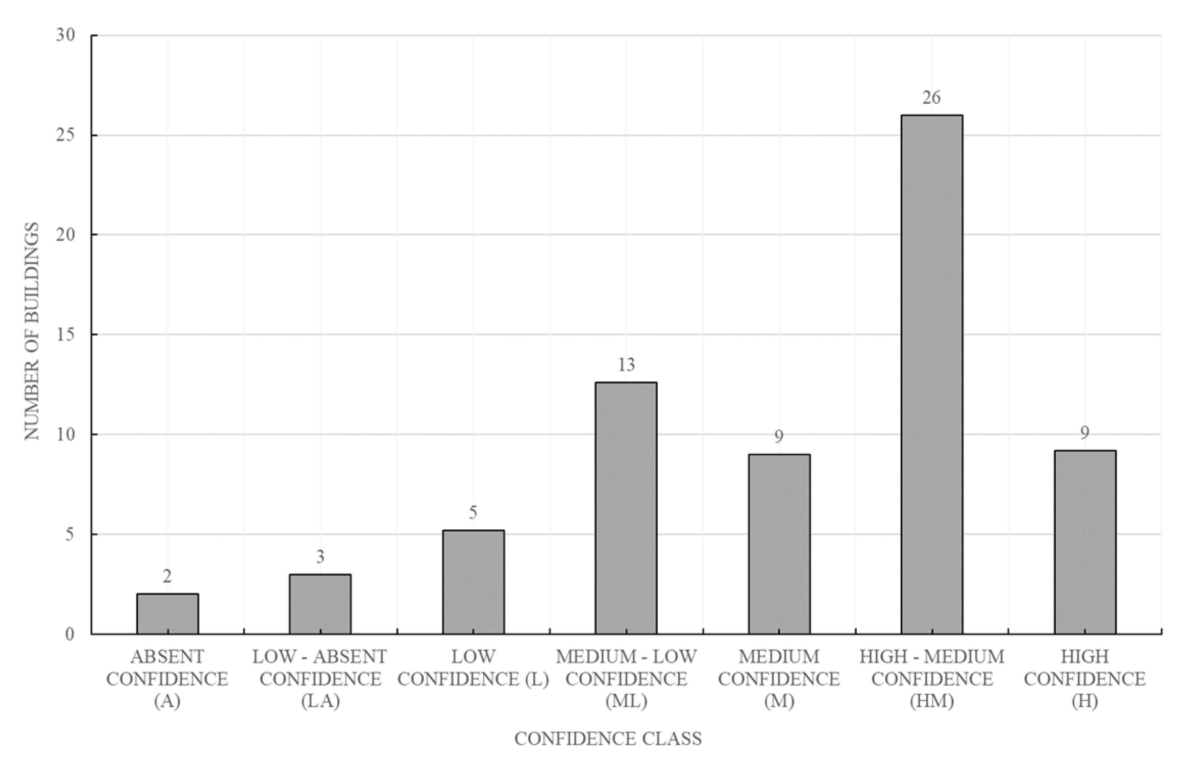
7. Introduction of the Information Quality (IQ) Index

The individual building’s vulnerability is influenced by the knowledge of the uncertainties related to considered parameters; the procedure before presented was therefore repeated introducing an Information Quality (IQ) index accounting for confidence level (CL) classes defined for the different parameters used in the I_V method. A 4-level confidence scale was developed based on the experience gained during the damage survey:

-

High confidence level (H): high information quality coming from complete (internal and external) surveys and direct measures on buildings including structures, materials, details, etc. High confidence in achieved data.

-

Medium confidence level (M): medium information quality, coming from external surveys on buildings and information rescued from historical/critical analysis or visual inspections. Medium confidence in achieved data resulted from direct/indirect measurements.

-

Low confidence level (L): external geometrical survey of the construction through satellite images integrated with considerations coming from buildings of similar typologies. Very low confidence in achieved data resulted from hypotheses not verified for the building or the urban setting.

Absent confidence level (A): information adopted with limited confidence or by random choice. The parameters’ class attribution is only indicative.

Three additional intermediate categories were introduced, with the aim of reducing the arbitrary choices of a class and providing an improved score assignment [45]: high-medium (HM), medium-low (ML) and low-absent (LA). The definition of a large number of confidence classes was related to the specific features of the constructions, characterized by high variability, and by the experience of the surveyor, that—as said—highly influences the outputs of I_V methods. Figure 19 shows the distribution of the CL in the case study; thanks to the different information collected and inspections carried out, more than 66% of the parameters resulted in a high-medium CL. In relation to assessed CL, a coefficient accounting for related uncertainties (UL) was determined (

Table 8. Uncertainty ranges and definition of the confidence classes.

Confidence Level (CL)	Percentage of Uncertainty (UL)
High Confidence (H)	0.0%
High-Medium Confidence (HM)	10.0%
Medium Confidence (M)	20.0%
Medium-Low Confidence (ML)	30.0%
Low Confidence (L)	40.0%
Low-No Confidence (LA)	50.0%
No Confidence (A)	60.0%

). The final CL for each class then resulted from the weighted average of the different CL ranges assigned to the buildings, neglecting the extreme cases with damage equal to D0–D1 or D5 according to EMS98 classification.

The level of uncertainty (UL) was applied to the weight of each parameter, determining the relevance (Δ) of the parameter for the seismic behaviour of the building, Equation (11).

$$\Delta =\frac{\sum {\mathrm{p}}_{\mathrm{i}}·\mathrm{UL}}{\sum {\mathrm{p}}_{\mathrm{i}}}$$

(11)

being p_i the weight of the i-th parameter and UL the corresponding uncertainty in relation to Table 8. The Δ value was used to increase or reduce the I_V defining a range where the vulnerability index expresses a correct result (11). These bounds can be seen as the transposition of the percentage of uncertainty coming from the evaluation of the parameters determining the I_V.

The range of numbers associated to each class was evaluated by checking whether the average of the damage detected $\left(\overline{{\mu }_R}\right)$ was within the upper $\left({\mu }_T^{+}\right)$ and lower bound $\left({\mu }_T^{-}\right)$ of the theoretical damage, assessed by increasing and reducing the I_V. The definition of the CL to be assigned to each class was defined through a step-by-step procedure, in which the uncertainty interval was calculated after assessing the vulnerability of each building (Figure 20).

$${\mathrm{I}}_{\mathrm{v}}=\{\begin{array}{c}\begin{array}{l}{\mathrm{I}}_{\mathrm{v}}^{-}=\sum {\mathrm{p}}_{\mathrm{i}}\left(1-\Delta \right)·{\mathrm{c}}_{\mathrm{i}}\to {\mathsf{\mu }}_{\mathrm{T}}^{-}\hspace{1em}\hspace{1em}\left(\mathrm{lower}\mathrm{bound}\right)\\ \hspace{1em}\hspace{1em}\overline{{\mathrm{I}}_{\mathrm{v}}}=\sum {\mathrm{p}}_{\mathrm{i}}·{\mathrm{c}}_{\mathrm{i}}\to \overline{{\mathsf{\mu }}_{\mathrm{T}}}\\ {\mathrm{I}}_{\mathrm{v}}^{+}=\sum {\mathrm{p}}_{\mathrm{i}}\left(1+\Delta \right)·{\mathrm{c}}_{\mathrm{i}}\to {\mathsf{\mu }}_{\mathrm{T}}^{+}\hspace{1em}\hspace{1em}\left(\mathrm{upper}\mathrm{bound}\right)\end{array}\end{array}$$

(12)

The use of the IQ index in the assessment of seismic vulnerability provided a range of possible values of I_V for each masonry building analysed. In this case study, the uncertainty classes used to describe the knowledge of the different Iv parameters, belong, on average, to the medium confidence class. When considering the upper and the lower bound I_V values, a new damage scenario was defined for the case study hit by the seismic intensity I_EMS98 = 7.65 ≈ 8.0 (Figure 21 and Figure 22). The line defining the average of the real damage overlapped the line of the mean theoretical damage “average calibrated”, thanks to the implemented weights’ calibration procedure. In this sense, the upper and lower bound allowed to better evaluate the expected damage of the single SU, while on average define the possible damage scenarios of the case study according to the EMS98 scale. Additionally in this case, the limitation of the mean damage formulation, Equation (3), in estimating high or low damage classes for different vulnerability values was evident: while real damage values are more scattered, the distribution of the estimated damage is concentrated around the average values. Figure 23 shows the relative error distribution considering all methods used, as well as the calibrated methods with and without the IQ index. The mean relative error between real and theoretical damage shifted from 0.49 (calibrated method) to 0.31 (calibrated method with IQ index).

8. Conclusions

Seismic vulnerability assessment methods, or Iv methods, based on statistical evaluations and damage observations are suitable tools for urban scale analysis; exploiting limited information and resources, they provide a first screening on the fragility of the area for a given seismic scenario. In this research, several well-accepted vulnerability index methods were studied and compared to verify their reliability in the estimation of damage scenarios, using as reference a case study hit by the recent 2016 Central Italy earthquake.

Results revealed the main limitations of these methods, and, as a whole, of statistical methods, i.e., their high dependence on the building characteristics and on the seismic scenario(s) originally used to calibrate and validate them. Another limitation is related to the definition of a single value for the vulnerability, which can potentially increase the difference between the real and expected/analytical damage.

The uncertainties related to the information quality of the survey were accounted for through a new parameter, the IQ index, analysing its influence on the variation of the I_V value. The obtained results revealed a difficulty in integrating this vulnerability assessment technique into a macroseismic method for the development of damage scenarios. It is important to note that a vulnerability assessment extended by two limiting conditions provides a greater awareness of the expected damage scenarios: if the results are distributed in a wide range, the survey has to be improved, giving a practical perspective to the IQ index. In this sense, the relative error between the theoretical and real damage has to be considered critically, paying attention to the reduction or increase of the damage level compared to the original data.

The estimated damage distribution is concentrated around the middle classes of the EMS98 scale, not allowing to consider low (D0) or high (D5) damage classes, even for very low or high vulnerabilities. This leads to an increase of the relative error between the theoretical and real damage, resulting from a sort of incorrect estimation of Bernardini’s formulation [31] and not by the vulnerability estimation itself. It shall also be underlined that the weights’ calibration is performed for a specific seismic intensity (I_EMS98 = 7.65 ≈ 8.0); the calibrated method is reliable for historical centres with the same construction typology, which, on average, is defined by a specific seismic vulnerability and hit by high seismic intensity (I_EMS98 ≈ 8.0). Most of the historical centres located in Central Italy, such as for example Assisi, L’Aquila [46] and Castelluccio di Norcia [47], present settlement configurations and building typologies similar to the case study. Their level of seismic hazard is also higher than the one in the case study analysed herein. Still, mathematical models can be a valid tool, when calibrated basing on real data, to achieve correct predictions.

As a final note, it is worth listing a few possibilities of future improvement of seismic vulnerability assessment approaches, namely by increasing the sample space of the data used for the statistical analysis, particularly in order to consider further seismic intensities and to consider other formulations for the definition of damage scenarios. In this sense, considering a large amount of data available, the Bayesian Linear Regression can be implemented in an artificial neural network (ANN) model [48]. For this application, the ANN must be trained to accurately understand the relationship between the damage level and the specific vulnerability index. According to the results achieved, a new analytical expression can be developed for the forecast of damage scenarios, and the issues related to the Bernardini et al. (2007) formulation [31] can be overcome.

References

1. Caprili, S.; Mangini, F.; Mussini, N.; Salvatore, W. Palazzo la sapienza in pisa: Structural assessment and retrofit of an historical masonry building in Italy. In ECCOMAS Congress 2016—Proceedings of the 7th European Congress on Computational Methods in Applied Sciences and Engineering; National Technical University of Athens: Athens, Greece, 2016; Volume 3, pp. 5230–5247. [Google Scholar]
2. Nazionale di Geofisica e Vulcanologia INGV. Archivio Storico Macrosismico Italiano (ASMI). 2019. Available online: https://emidius.mi.ingv.it/ASMI/ (accessed on 12 March 2020).
3. Dolce, M.; Masi, A.; Samela, C.; Santarsiero, G.; Vona, M.; Zuccaro, G.; Cacace, F.; Papa, F. Examination of typological and damaging characteristics of the built heritage of San Giuliano di Puglia (in Italian). In Proceedings of the XI Italian Congress “L’Ingegneria Sismica in Italia” (ANIDIS), Genova (Palazzo Ducale), Italy, 25–29 January 2004. [Google Scholar]
4. Formisano, A.; Grippa, M.R.; Di Feo, P. L’Aquila earthquake: A survey in the historical centre of Castelvecchio Subequo. In Proceedings of the COST ACTION C26: Urban Habitat Constructions under Catastrophic Events, Neaples, Italy, 16–18 September 2010; pp. 371–376. [Google Scholar]
5. Borghini, A.; Del Monte, E.; Ortolani, B.; Vignoli, A. Studio del danno causato dal sisma del 06/04/2009 alla frazione di Castelnuovo Comune di San Pio delle Camere (Aq). In Proceedings of the XIV Convegno Nazionale Anidis L’Ingegneria Sismica In Italia, Bari, Italy, 18–22 September 2011. [Google Scholar]
6. Borri, A.; Sisti, R.; Zaroli, A.; Prota, A.; Di Ludovico, M.; De Maria, A. Gli edifici di Campi Alto di Norcia nel sisma del 2016. Diversità nella risposta sismica di costruzioni consolidate in anni recenti. Structural 200 2018, 218, 1–27. [Google Scholar]
7. MIBACT. Linee Guida per la Valutazione e Riduzione del Rischio Sismico del Patrimonio Culturale Allineate alle Nuove Norme Tecniche per le Costruzioni; Gangemi: Roma, Italy, 2010. [Google Scholar]
8. Cattari, S.; Frumento, S.; Lagomarsino, S.; Resemini, S. Multi-level procedure for the seismic vulnerability assessment of masonry buildings: The case of Sanremo (north-western italy). In Proceedings of the First European Conference on Earthquake Engineering and Seismology, Geneve, Switzerland, 3–8 September 2006. [Google Scholar]
9. Ortega, J.; Vasconcelos, G.; Rodrigues, H.; Correia, M.; Ferreira, T.M.; Vicente, R. Use of post-earthquake damage data to calibrate, validate and compare two seismic vulnerability assessment methods for vernacular architecture. Int. J. Disaster Risk Reduct. 2019, 39, 101242. [Google Scholar] [CrossRef]
10. D’Ayala, D.; Spence, R.; Oliveira, C.; Pomonis, A. Earthquake loss estimation for Europe’s historic town centres. Earthq. Spectra 1997, 13, 773–793. [Google Scholar] [CrossRef]
11. Cattari, S.; Curti, E.; Giovinazzi, S.; Lagomarsino, S.; Parodi, S.; Penna, A. Un modello meccanico per l’analisi di vulnerabilità del costruito in muratura a scala urbana. In Proceedings of the XI Congresso ANIDIS “L’Ingegneria Sismica in Italia”, Genova (Palazzo Ducale), Italy, 25–29 January 2004. [Google Scholar]
12. Ferreira, T.M.; Maio, R.; Vicente, R. Analysis of the impact of large scale seismic retrofitting strategies through the application of a vulnerability-based approach on traditional masonry buildings. Earthq. Eng. Eng. Vib. 2017, 16, 329–348. [Google Scholar] [CrossRef]
13. Novelli, V.I.; D’Ayala, D.; Makhloufi, N.; Benouar, D.; Zekagh, A. A procedure for the identification of the seismic vulnerability at territorial scale. Application to the Casbah of Algiers. Bull. Earthq. Eng. 2015, 13, 177–202. [Google Scholar] [CrossRef] [Green Version]
14. Blyth, A.; Di Napoli, B.; Parisse, F.; Namourah, Z.; Anglade, E.; Giatreli, A.M.; Rodrigues, H.; Ferreira, T.M. Assessment and mitigation of seismic risk at the urban scale: An application to the historic city center of Leiria, Portugal. Bull. Earthq. Eng. 2020, 18, 2607–2634. [Google Scholar] [CrossRef]
15. Ramos, L.F.; Lourenço, P.B. Modeling and vulnerability of historical city centers in seismic areas: A case study in Lisbon. Eng. Struct. 2004, 26, 1295–1310. [Google Scholar] [CrossRef] [Green Version]
16. Lagomarsino, S.; Penna, A.; Galasco, A.; Cattari, S. TREMURI program: An equivalent frame model for the nonlinear seismic analysis of masonry buildings. Eng. Struct. 2013, 56, 1787–1799. [Google Scholar] [CrossRef]
17. AIMS. “SERA TA Project # 19”. 2019. Available online: https://sera-ta.eucentre.it/sera-ta-project-19/ (accessed on 20 August 2020).
18. Calvi, G.M.; Pinho, R.; Magenes, G.; Bommer, J.J.; Restrepo-Vélez, L.F.; Crowley, H. Development of Seismic Vulnerability Assessment Methodologies over the Past 30 Years. ISET J. Earthquake Technol. 2006, 43, 75–104. [Google Scholar]
19. Kassem, M.M.; Mohamed Nazri, F.; Noroozinejad Farsangi, E. The seismic vulnerability assessment methodologies: A state-of-the-art review. Ain Shams Eng. J. 2020. [Google Scholar] [CrossRef]
20. Fajfar, P. Capacity spectrum method based on inelastic demand spectra. Earthq. Eng. Struct. Dyn. 1999, 28, 979–993. [Google Scholar] [CrossRef]
21. GDNT. Manuale per il Rilevamento della Vulnerabilità Sismica Degli Edifici; Dipartimento Protezione Civile. Available online: http://gndt.ingv.it/Strumenti/Schede/Schede_vulnerabilita/scheda_secondo_livello_mur.pdf (accessed on 29 October 2020).
22. Formisano, A.; Landolfo, R.; Mazzolani, F.M.; Gilda, F. A quick methodology for seismic vulnerability assessment of historical masonry aggregates. In Proceedings of the COST C26_Final Conference “Urban Habitat Constructions under Catastrophic, Neaples, Italy, 26 October 2014. [Google Scholar]
23. Ferreira, T.M.; Vicente, R.; Varum, H. Vulnerability assessment of building aggregates: Macroseimic A macroseimic approach. In Proceedings of the 15th World Conference on Earthquake Engineering, Lisboa, Portugal, 24–28 September 2012. [Google Scholar]
24. Carlin, B.B.P.; Louis, T.A. Bayesian Data Analysis By A. Gelman, J. B. Carlin, H. S. Stern, and D. B. Rubin. Am. J. Epidemiol. 1997, 146, 21–24. [Google Scholar]
25. INGV. Sequenza Sismica tra le Province di Rieti, Ascoli P., Perugia, Teramo e L’Aquila. INGV—Terremoti. 2016. Available online: https://web.archive.org/web/20160827124928/http://terremoti.ingv.it/it/ultimi-eventi/1001-evento-sismico-tra-le-province-di-rieti-e-ascoli-p-m-6-0-24-agosto.html (accessed on 2 September 2020).
26. INGV. Sequenza Sismica in Italia Centrale: Nuovo Evento di Magnitudo 6.5, 30 ottobre 2016, ore 07:40. INGV—Terremoti. 2016. Available online: https://ingvterremoti.com/2016/10/30/sequenza-sismica-in-italia-centrale-nuovo-evento-di-magnitudo-6-5-30-ottobre-2016-ore-0740/ (accessed on 2 September 2020).
27. Meletti, C.; Visini, F.; D’Amico, V.; Rovida, A. Seismic hazard in Central Italy and the 2016 amatrice earthquake. Ann. Geophys. 2016, 59. [Google Scholar] [CrossRef]
28. Baggio, C.; Bernardini, A.; Livio, R.C.; Bella, M.; Pasquale, G.D.; Agostino, M.D.; Giampiero, A.M.; Zuccaro, G. Field Manual for Post-Earthquake Damage and Safety Assessment and Short Term Countermeasures (AeDES); Office for Official Publications of the European Communities: Bruxelles, Belgium, 2007. [Google Scholar]
29. Grünthal, G. European Macroseismic Scale 1998 EMS-98 Editor; European Centre for Geodynamics and Seismology: Luxembourg, 1998. [Google Scholar]
30. Benedetti, D.; Petrini, V. Sulla vulnerabilita sismica di edifici in muratura: Un metodo di valutazione. A method for evaluating the seismic vulnerability of masonry buildings. L’industria Costr. 1984, 149, 66–74. [Google Scholar]
31. Bernardini, A.; Giovinazzi, S.; Lagomarsino, S.; Parodi, S. Vulnerabilità e previsione di danno a scala terri- toriale secondo una metodologia macrosismica coerente con la scala EMS-98. In Proceedings of the XII Congresso ANIDIS “L’ingegneria Sismica in Italia”, Pisa, Italy, 10–14 June 2007. [Google Scholar]
32. Barbat, A.H.; Pujades, L.G.; Lantada, N. Seismic damage evaluation in urban areas using the capacity spectrum method: Application to Barcelona. Soil Dyn. Earthq. Eng. 2008, 28, 851–865. [Google Scholar] [CrossRef]
33. Vicente, R.; Parodi, S.; Lagomarsino, S.; Varum, H.; Silva, J.A.R.M. Seismic vulnerability and risk assessment: Case study of the historic city centre of Coimbra, Portugal. Bull. Earthq. Eng. 2011, 9, 1067–1096. [Google Scholar] [CrossRef]
34. Cherubini, A.; Corazza, L.; Di Pasquale, G.; Dolce, M.; Martinelli, A.; Petrini, V. Censimento di Vulnerabilità degli Edifici Pubblici, Strategici e Speciali nelle Regioni Abruzzo, Basilicata, Calabria, Campania, Molise, Puglia e Sicilia—Cap. 4: Risultati del Progetto; Protezione Civile, D., Ed.; Cap.4. Rom.; ROMA: Rome, Italty, 1999. [Google Scholar]
35. Vicente, R. Strategies and Methodologies for Urban Rahabilitation Interventions; University of Aveiro, University Press: Aveiro, Portugal, 2010. [Google Scholar]
36. Sandi, H.; Floricel, I. Analysis of the seismic risk affecting the existing IX building stock. In Proceedings of the 10th European Conference on Earthquake Engineering, Vienna, Austria, 28 August–2 September 1995; Volume 3, pp. 1105–1110. [Google Scholar]
37. Galli, P.; Castenetto, S.; Peronace, E. Rapporto Sugli Effetti Macrosismici del Terremoto del 30 Ottobre 2016 (Monti Sibillini) in Scala MCS. Available online: https://emidius.mi.ingv.it/ASMI/study/GALAL016a (accessed on 29 October 2020).
38. Musson, R.M.W.; Cecić, I. Chapter 12 Intensity and Intensity Scales; Helmholtz Zentrum: Potsdam, Germany, 2011. [Google Scholar] [CrossRef]
39. Margottini, C.; Molin, D.; Serva, L. Intensity versus ground motion: A new approach using Italian data. Eng. Geol. 1992, 33, 45–58. [Google Scholar] [CrossRef]
40. Spence, R.; Bommer, J.; Del Re, D.; Bird, J.; Aydinoǧlu, N.; Tabuchi, S. Comparing loss estimation with observed damage: A study of the 1999 Kocaeli earthquake in Turkey. Bull. Earthq. Eng. 2003, 1, 83–113. [Google Scholar] [CrossRef]
41. Lancaster, T. An Introduction to Modern Bayesian Econometrics; Blackwell Pub.: Hoboken, NJ, USA, 2004; ISBN 9781405117203. [Google Scholar]
42. Haario, H.; Saksman, E.; Tamminen, J. Adaptive proposal distribution for random walk Metropolis algorithm. Comput. Stat. 1999, 14, 375–395. [Google Scholar] [CrossRef]
43. Marelli, S.; Sudret, B. UQLab: A Framework for Uncertainty Quantification in Matlab. In Proceedings of the Second International Conference on Vulnerability and Risk Analysis and Management (ICVRAM) and the Sixth International Symposium on Uncertainty, and Analysis (ISUMA), Modeling, Liverpool, 13–16 July 2014. [Google Scholar]
44. Ferreira, T.M.; Maio, R.; Costa, A.A.; Vicente, R. Seismic vulnerability assessment of stone masonry façade walls: Calibration using fragility-based results and observed damage. Soil Dyn. Earthq. Eng. 2017, 103, 21–37. [Google Scholar] [CrossRef]
45. Ferreira, T.M.; Rodrigues, H.; Vicente, R. Seismic Vulnerability Assessment of Existing Reinforced Concrete Buildings in Urban Centers. Sustainability 2020, 12, 1996. [Google Scholar] [CrossRef] [Green Version]
46. Indirli, M.; Kouris, L.A.S.; Formisano, A.; Borg, R.P.; Mazzolani, F.M. Seismic Damage Assessment of Unreinforced Masonry Structures After The Abruzzo 2009 Earthquake: The Case Study of the Historical Centers of L’Aquila and Castelvecchio Subequo. Int. J. Archit. Herit. 2013, 7, 536–578. [Google Scholar] [CrossRef]
47. Marchetti, L. Vulnerability of Historic Centres and Cultural Heritage. Available online: https://emidius.mi.ingv.it/GNDT2/Att_scient/Pe2001_RelAnn/Marchetti/PE2001_RelAnn_Marchetti_eng (accessed on 29 October 2020).
48. Ferreira, T.M.; Estêvão, J.; Maio, R.; Vicente, R. The use of Artificial Neural Networks to estimate seismic damage and derive vulnerability functions for traditional masonry. Front. Struct. Civ. Eng. 2020, 14, 609–622. [Google Scholar] [CrossRef]
Figure 1. Methodological framework adopted in the present work.
Applsci 11 00849 g001
Figure 2. (a) View of Campi Alto di Norcia after the 2016 earthquakes; (b) identification of structural units, highlighted in red and identified with different IDs, within Campi.
Applsci 11 00849 g002
Figure 3. Schematic representation of a typical structural aggregate (SA25 is shown) in Campi Alto di Norcia.
Applsci 11 00849 g003
Figure 4. Histogram (a) and map (b) of the distribution of the floor number for each SU in Campi Alto di Norcia. Horizontal storeys and roof typologies.
Applsci 11 00849 g004
Figure 5. (a) Distribution of floor’s typology; (b) distribution of the roof typology.
Applsci 11 00849 g005
Figure 6. Mapping of the damage observed in Campi Alto di Norcia, according to the European Macroseismic Scale (EMS)98.
Applsci 11 00849 g006
Figure 7. Comparison between the damage level and different retrofit typologies carried out before the seismic.
Applsci 11 00849 g007
Figure 8. Vulnerability classes distribution of the different parameters, according to (a) the GDNT method, (b) the Formisano method and (c) the Vicente method.
Applsci 11 00849 g008
Figure 9. IV distribution in the case study according to (a) the GDNT method, (b) the Formisano method and (c) the Vicente method.
Applsci 11 00849 g009
Figure 10. Normalized IV distribution in the case study of Campi Alto di Norcia, according to (a) the GDNT method, (b) the Formisano method and (c) the Vicente method.
Applsci 11 00849 g010
Figure 11. (a) Distribution of the IV through the different methods for 67 SUs; (b) distribution of the IV through the different methods for 50 SUs in the aggregate.
Applsci 11 00849 g011
Figure 12. Procedure adopted to evaluate the reliability of vulnerability assessment methods.
Applsci 11 00849 g012
Figure 13. Relative error distribution of the IV methods obtained from (a) the direct measure and (b) the full sample range, where in red the reliability of the Vicente method is highlighted.
Applsci 11 00849 g013
Figure 14. Comparison between the real damage detected in the case study and the theoretical damage evaluated through different vulnerability methodologies for each SU.
Applsci 11 00849 g014
Figure 15. Comparison between the real damage detected in the case study (a) and the theoretical damage scenarios evaluated through (b) the GDNT, (c) the Vicente and (d) the Formisano method for each SU.
Applsci 11 00849 g015
Figure 16. Vulnerability curves of the case study for different seismic intensities using the IV methods selected; the damage and the intensity of the seismic events of October 2016 are highlighted in red, through the damage detected after the seismic emergency. Starting from the latter, the real damage is extended to other seismic intensities through the Bernardini et al. (2007) formulation [31].
Applsci 11 00849 g016
Figure 17. Procedure followed for the identification of the weight distribution.
Applsci 11 00849 g017
Figure 18. Comparison between the original and the calibrated results.
Applsci 11 00849 g018
Figure 19. Distribution of the confidence classes in the case study.
Applsci 11 00849 g019
Figure 20. Step by step procedure for the LC definition of each confidence class.
Applsci 11 00849 g020
Figure 21. Comparison between real damage and the theoretical damage evaluated through the calibrated method considering the Information Quality (IQ) index. The grey area defines in average the possible damage scenarios of the case study according to the EMS98 scale.
Applsci 11 00849 g021
Figure 22. Comparison between (a) the damage scenarios of the case study detected after the 2016 seismic events, (b) the damage scenarios evaluated with the Vicente method and (c) with the calibrated method, considering the IQ index.
Applsci 11 00849 g022
Figure 23. Relative error distribution of the IV methods obtained from the direct measure considering (a) the calibrated method and (b) the calibrated method with the IQ index. The grey area defines the confidence bounds for expected damage scenarios, i.e., the range of the relative error of the building stock analysed is on average between 0.3 and 0.7.
Applsci 11 00849 g023