Abstract
In the non-free-field, with the effect of reflection sounds from the reflection boundary, the vibration character of a submerged structure often changes, which may have significant influences on the measurement system configurations. To reduce the engineering cost in low-frequency sound prediction of a submerged structure with finite depth, two methods based on the theory of acoustic radiation mode (ARM) are proposed. One is called the vibration reconstruction equivalent source method (VR-ESM), which utilizes the ARM to reconstruct the total vibration of the structure, and the sound prediction is completed with the equivalent source method (ESM); the other is called the compressed modal equivalent source method (CMESM), which utilizes the theory of compressive sensing (CS) and the ARM to reinforce the sparsity of source strengths. The sound field separation (SFS) technology is combined with the above two methods for constructing the ARMs accurately in the non-free field. Simulations show that both methods are efficient. Compared with the traditional method based on the structural modal analysis, the methods based on the ARM could efficiently reduce the scale of the measurement system. However, the measurement point arrangement should be optimized to keep the prediction results accurate. In this paper, the optimization process is completed with the efficient independence (EFI) method. In addition, some factors that may affect the prediction accuracy are also analyzed in this paper. When the submerge depth is large enough, the process of contrasting ARMs could be further simplified. The results of the paper could help in saving engineering costs to predict the low-frequency sound radiation of submerged structures in the future.
1. Introduction
The sound prediction method of underwater structures has been widely concerned by scholars in various countries as it could provide important prior information for self-noise monitoring and active noise controlling of submerged vehicles. Especially, the sound radiation of underwater vehicles does not often satisfy the free-field condition, which means that the reflection sounds from boundaries and scattering sounds could make a significant contribution to the sound radiation, according to the study of Chen [1]. As analytical methods could hardly be applied for complex structures and acoustical environments, several numerical calculation methods have been developed to be applied for the sound prediction in non-free fields, such as the finite element method (FEM), the boundary element method (BEM), the combination of FEM and BEM (FEM–BEM), and the element radiation superposition method (ERSM) [2,3,4,5,6]. However, the methods have their own disadvantages, which are analyzed sufficiently in the study of Wang [7]. For example, the details of excitation force are required in advance for FEM and FEM–BEM, which is impractical in engineering applications. Though BEM could accomplish the prediction with measurement data, the singular integrals could be an obstacle for fast prediction. Though ERSM has an obvious advantage in computational efficiency, its usage could hardly be flexible in complex acoustic environments.
Koopmann et al. first proposed the equivalent source method (ESM) to calculate the sound radiation of structure [8]. Li and Huang et al. analyzed the stability of the equivalent source method and the factors affecting the calculation accuracy of ESM and found that ESM not only avoids the problem of singular integral, but also has higher computational efficiency compared with the commonly used numerical methods such as BEM [9,10]. Using the complex vector radius method, Xiang et al. found that the non-uniqueness of the solution of ESM at singular frequencies could be avoided, which broadens the application of ESM [11]. Moreover, by modifying the transfer function, scholars have studied the sound field prediction of structures in the non-free field, and obtained many significant conclusions [12,13,14]. When ESM is used to predict the sound field of structure, the input is often chosen to be the vibration of the structure surface. In the study of [15], Shang combined ESM with FEM to solve the difficulty of obtaining the vibration of the structure in a complex environment, and the sound prediction of an elastic cylindrical shell in idealized waveguide is completed. However, there was no further study on the measurement point arrangement in the above research. Most previous studies chose uniform measurement point arrangement for convenience. The denser the measurement points, the higher the prediction accuracy and the computational cost [7]. In the studies of Wang and Tao et al., they found that the measurement point arrangements are closely linked with the structural vibration mode (SVM) [7,16]. Zhang proposed a method based on the dominantly radiated structural mode (DRSM) to calculate the sound power of a cylindrical shell [17]. As the mutual coupling among the modes at low frequencies could be ignored, the number of measurement points could be reduced. However, the method is only efficient in predicting the sound power of the structure. Meanwhile, for a structure with a complex shape or big size, the structural vibration mode could be quite complex, which limits the application of SVM.
Photiadis and Borgiotti put forward the concept of the acoustic radiation mode (ARM) [18,19]. From the perspective of sound power, the sound pressure in the sound field is expressed as a set of orthogonal basis functions. Each order of ARM is independent, without coupling among SVMs. Therefore, the control and calculation of sound power could be very simple. In the studies of [20,21,22,23,24], scholars designed a series of basis functions of ARMs using the radiated sound power matrix and completed the calculation of ARMs and the reconstruction of the sound field. Nie and Zhan et al. introduced ESM into the application of ARM and conquered the difficulty of solving the radiation sound impedance on the vibrating bodies [25,26]. The theory of ARM is widely used in the nearfield acoustic holography (NAH), source localization, and sound field reconstruction. Efren, Bi, and Jᴓrgen et al. have proven that the expansion coefficients of the orthogonal bases may have high sparsity when combining ARM with ESM [27,28,29]. Based on the theory of compressed sensing (CS), the sound field reconstruction of structural sound source can be accomplished with sparse measurement points. Li, Su, and Mao et al. discussed the optimization methods of measurement systems based on ARM and found that, with non-uniform distribution of measurement points, the accuracy of sound reconstruction could be higher [30,31,32]. However, all the above studies were carried out in the free field. The studies in the non-free-field deserve more attention. With the maturity of the sound field separation technology (SFS), the sound reconstruction and prediction in the non-free-field are more convenient. In the NAH theory based on ESM, several methods could be applied to separate the real sources from the disturbed sources such as the double-layer sound pressure measurement method, double-layer particle velocity measurement method, and single-layer sound pressure-particle velocity measurement method. In fact, in the non-free-field, the strengths of real sources could also be obtained with SFS based on the structural vibration [1,33]. Thus, the discussion about the optimization of measurement system in non-free-field could be completed.
In this paper, two methods based on the theory of ARM are proposed to predict the sound radiation of an elastic structure with finite submerge depth. SFS is used to construct the ARMs accurately when the reflection sounds have a significant influence on the structural vibration. Generally, the measurement point arrangement should change as the existence of the reflection sounds changes the details of SVM. Regretfully, the quantity of measurement points still is limited by the Nyquist sampling rule. However, according to the good convergence of ARM, the quantity of measurement points could be invariant and further reduced. In spite of this, the ill-condition problem of the sensing matrices may lead to large prediction errors and should be avoided. With the help of EFI, the measurement point arrangement could be optimized by reducing the condition numbers of the sensing matrices and the accuracy of prediction could be improved. Furthermore, some other factors such as the frequency, the signal–noise ratio (SNR), and the submerged depth, which may affect the prediction accuracy, are analyzed in the paper. When the submerged depth is large enough, the process of prediction could be simplified with a ‘quick case’ because the effect of reflection sounds on the structural vibration could be neglected. In order to illustrate the paper more clearly, a flowchart is given out as Figure 1.
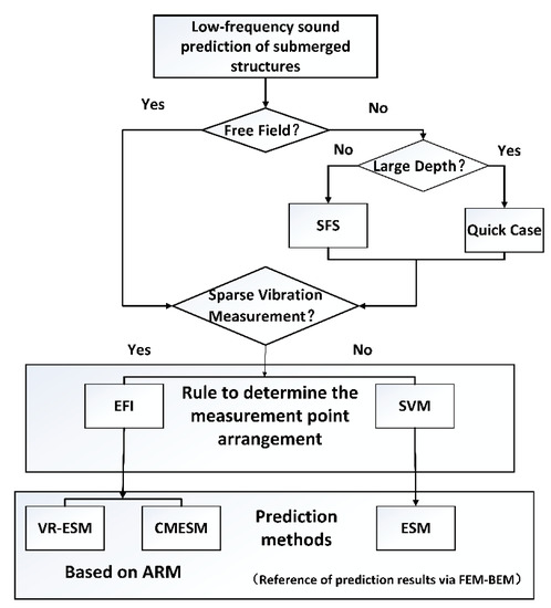
Figure 1.
The flowchart illustrating the methodology of the paper. SFS, sound field separation; EFI, efficient independence; SVM, structural vibration mode; VR-ESM, vibration reconstruction equivalent source method; CMESM, compressed modal ESM; ARM, acoustic radiation mode; FEM, finite element method; BEM, boundary element method.
In Section 2, the theoretical bases of the prediction methods such as ESM, CMESM, and VR-ESM will be presented. The method of SFS will also be introduced to apply for the sound prediction in the half-space. Then, in Section 3, some numerical simulations will be carried out to manifest the efficiency of CMESM and VR-ESM. The results of ESM are regarded as the references to highlight the advantages of CMESM and VR-ESM to enhance the sparsity of the measurement system. Meanwhile, the necessity of EFI to optimize the measurement system will be confirmed. In Section 4, some factors that could affect the prediction results will be discussed briefly. Finally, the conclusions of the paper will be given out in Section 5.
2. Theoretical Basis
2.1. Equivalent Source Method (ESM)
Considering an arbitrarily-shaped complex structure submerged in homogenous fluid medium, the pressure and the particle velocity at any field point could be represented as the superposition of sound field generated by a series of point sources distributed on a virtual surface inside the structure [8]:
where is the density of the medium; , is the angular frequency; is the number of equivalent sources; and is the strength of the th equivalent source, which is located at the position of . Xiang et al. indicated that the form of a single equivalent source could be various, such as monopole, dipole, or the combination of monopole and dipole [11]. However, using monopole as the form of equivalent source has an obvious advantage because the transfer function could be obtained easily even in a non-free field. is the transfer function (Green’s function), given by the following:
where is the wavenumber. If the structure is submerged in the water with finite depth, the reflection sounds from the water–air boundary should not be ignored. Thus, the expression of could be rewritten as follows:
where is the reflection coefficient of the boundary and is the mirror of the equivalent source located at the position of . Generally, the water–air boundary is regarded as a soft boundary and . Moreover, the normal velocity on the surface of the structure could be reconstructed by the equivalent sources:
where is the normal vector on the surface node located at . The matrix expression of Equation (4) is as follows:
where is referred to as the dipole matrix, . Given that there are measurement points on the surface of the structure, is the column vector that contains the normal velocities at the measurement points, and is the column vector that contains the equivalent source strengths. is not a square matrix and is satisfied in ESM. Thus, the Moore–Penrose pseudoinverse is necessary to perform the matrix inversion. Once the equivalent sources are configured, the strength of equivalent sources could be obtained with Equation (5).
where the superscript ‘+’ denotes the Moore–Penrose pseudoinverse, , and the superscript ‘H’ denotes the Hermite transposition. Equation (6) describes the solution of overdetermined equations. Thus, the approximate solution of the unknown source strength vector is often solved with minimum -norm via the minimization problem [34]:
When the interference of noise could not be ignored, the Tikhonov regularization is usually chosen to avoid the ill-posed inverse problem, which is caused by the poorly conditioned dipole matrix [35]. Thus, Equation (7) could be rewritten as follows:
where is the regularization parameter. It is essential to acquire accurate equivalent source strengths for sound prediction with high efficiency. Particularly, the reflection sounds could make a significant contribution to the structural vibration in the non-free-field, which makes the solution of equivalent source strengths computationally costly [36]. In the work [1], Chen proposed a method to separate the normal velocity on the surface of the structure, which could make a contribution to the radiation sound field. With the method, the ‘useful’ strength of equivalent sources could be calculated with the normal derivative of free Green’s function, which simplifies the computation.
2.2. Sound Field Separation Technology Based on Vibration Measurement
When a structure is located in the non-free-field, the reflection sounds could change the vibration of the structure. In NAH based on ESM, the interference of the reflection sounds must be excluded to obtain the ‘useful’ strength of equivalent sources in the free field. Most relevant studies chose double sound pressure holographic layers, double particle velocity holographic layers, or single sound pressure-particle velocity holographic layer to complete the process of SFS [36,37,38]. However, with the above methods, the scale of the measurement system would be quite enormous. In this section, the separation of normal velocity on the structural surface based on SFS will be introduced [1].
Suppose that the structure is submerged in the water with a finite depth. In that case, only the reflection sounds from the water–air boundary need to be considered. The schematic diagram of the ESM in half-space could be shown in Figure 2.
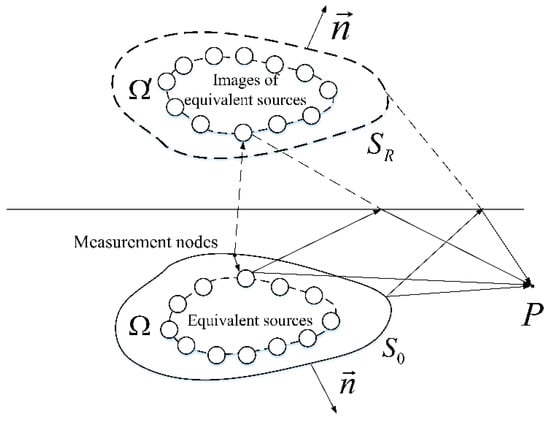
Figure 2.
The schematic diagram of the equivalent source method in half-space.
In the figure, is the surface of the structure, SR is the ‘image surface’ of the virtual structure, is the surface of equivalent sources, while is the surface of image equivalent sources. The measured normal velocity on the structural surface consists of three parts: the normal velocity in the free field , the normal velocity caused by reflection sounds , and the normal velocity related to the scattering sounds :
Obviously, the radiated sounds and scattering sounds are the components that radiate outwards, while the reflection sounds radiate inwards. The strength of equivalent sources could be also divided into three parts, which are related to the above three vibration components: ,, and. As ESM is based on the Huygens’ principle, which has been proven to be equivalent to the Helmholtz integral Equation [7], it could be easily concluded that does not make contribution to the radiated sound field:
where is the location of the node on and is the sound pressure variation caused by reflection sounds on . Thus, to precisely predict the radiated sound of a structure in half-space, should be separated from the measured normal velocity . For simplicity, the normal derivative is rewritten as . With Equations (5) and (9), the vibration components could be written as follows:
The relationship between and is as follows:
Then, the ‘useful’ normal velocity could be separated from to calculate the strength of the equivalent sources:
where is an identity matrix with dimensions. With the technology of SFS, it is not necessary to solve the normal derivative of non-free Green’s function to obtain the ‘useful strength’ of equivalent sources . Thus, the process of calculation could be simplified.
2.3. The Sound Prediction Based on ARM
From Equation (7), it could be seen that, when calculating the equivalent source strength in the ESM, the measurement points should not be less than the equivalent sources. Considering the engineering cost, it is important to reduce the quantity of measurement points for the sound prediction. As the ARM has been proven to have good convergence with the increase of ARM order, it offers possibility to reduce the scale of the measurement system [31]. Based on the theory of ARM, two methods could be designed to apply for the sound prediction. One is combined with the theory of compressed sensing (CS), which is called the CMESM [28]. The other is combined with the reconstruction of structural vibration, which is called the VR-ESM for convenience. Both methods are modified with the SFS to construct the ARMs more accurately when the influences of reflection sounds on the structural vibration could not be neglected.
Firstly, the theory of ARM should be introduced briefly. ARM explain the sound radiation of a structure from the perspective of sound power . In the work [38], Liu gave out the relationship between the sound power and the equivalent source strengths:
where is the power resistance matrix and the expression of in free field is as follows:
where is the sinc function and , is the distance between the ith and the jth equivalent sources. Obviously, is a real symmetric matrix. Using the eigenvalue decomposition, could be expressed as follows:
where is a real diagonal matrix of the eigenvalues that are listed in descending order, and is an orthogonal matrix composed of eigenvectors that contains an orthogonal basis of -dimensional space. The column vectors of are regarded as the equivalent source ARMs. Bi proposed the CMESM to reduce the scale of the measurement system on the holographic surface [28]. The usage of ARM in the theory of CMESM enhances the sparsity of equivalent source strengths and makes the sparsity of measurement points possible. Still, it could break through the limit of Nyquist sampling law. CMESM is able to reconstruct the sound field generated by a sound source with arbitrary shape and has less limitation to the sparsity of true source distribution.
The power resistance could be different for the half-space from the free field when the effect of reflection sounds could not be neglected. As derives from the interactions among the equivalent sources [25], it could fall to three categories: the power resistance related to the equivalent sources inside the real structure , the power resistance related to the image equivalent sources inside the virtual structure , and the mutual power resistance related to the interactions among the equivalent sources and their mirrors . Thus, the total radiated sound power consists of four components:
where is the sound power derived from the equivalent sources inside the structure, is the sound power derived from the image equivalent sources inside the virtual structure, and and are the sound power components derived from the interactions among the equivalent sources and their images. According to the Helmholtz integral, when the sound source is not inside a closed surface, the integral of the source strength on the surface makes no contribution to the total sound field [1]. It is easy to find that, in Equation (17), and are the components that make no contribution to the sound radiation. Therefore, when reconstructing or predicting the sound field, only and need to be considered. Meanwhile, is equal to because of the mirror–image relationship. The strength of equivalent sources could be expanded by the orthogonal basis:
where the vector is the th equivalent source ARM and and are the expansion coefficients for the th ARM. When the measurement points are sparse, Equation (18) could be solved with the minimum -norm [28]:
where is the sensing matrix with the dimension of , and it is possible that . Equation (19) is the basic formulation of CMESM; the sparse basis is used here to compress the equivalent source strengths for reinforcing the sparsity of the solution. Thus, the measurement points could be far less than the equivalent sources. In the study [39], Chardon defined as a function of the hologram norm, and , and the optimal value of is determined by the cross-validation method.
If the structure is located in the half-space, according to the SFS, could be separated into two parts: , which is related to the equivalent sources inside the structure, and , which is related to the mirror equivalent sources. Equation (19) could be rewritten as below:
where . Equation (20) is a convex optimization problem solved with the CVX package in this paper [40] and is a parameter related to the sound–noise ratio. The sound pressure in the sound field could be expressed by the ARMs [25]:
It should be noted that the ill-condition problem of and could be quite severe, which may lead to the ill-condition problem of the sensing matrices. Therefore, even a tiny change of could lead to obvious variation to the solution of . Bi solved the problem by arranging the measurement randomly, where blindness exists in engineering applications. Moreover, the ill-condition problem could be improved by increasing the quantity of measurement points, which weakens the advantage of the method [28]. Thus, when the quantity of measurement points is fixed, the measurement arrangement should be optimized to avoid the ill-condition problem of sensing matrices. As the CMESM is not able to present the ARM form of the normal velocities, the VR-ESM is put into effect for establishing the ARMs of normal velocity. Meanwhile, the EFI is used for optimization of the measurement system.
With Equations (5) and (14), the sound power of could be rewritten as follows:
where . For the half-space, the expression of is as follows:
where is a positive definite Hermite matrix whose real part is a real symmetric matrix, which could be expressed as the form of eigenvalue decomposition according to the study of Zhan et al. [26], . Unitary matrix is composed of a series of orthogonal column vectors, which are regarded as velocity ARMs and sorted by the eigenvalues. Therefore, could be expressed as follows:
where is the expansion coefficient column vector of ARMs. As Equation (24) has good convergence with the increase of ARM order, it could be rewritten as follows: , where is the ARM truncation number. In the process, should be guaranteed. Suppose that only points could be regarded as measurement points from the measurement points to be selected, the normal velocities at these points could be expressed as follows: . Generally, the quantity of measurement points should not be less than the truncation number, . Thus, the relationship between and could be written as follows:
It should be noted that the column vectors of are not orthogonal any more. Equation (25) means that total vibration of the structure could be reconstructed by the vibration measured at sparse points. If the total vibration is reconstructed accurately enough, the prediction of sound field is also accurate with the ESM. However, Equation (20) is an inverse problem and the condition number of the sensing matrix should be limited to avoid the ill-condition problem. Su proposed a method based on the EFI to optimize the measurement point arrangement [31]. A matrix for measuring the linear-independence contribution of the measurement points to the sensing matrix is defined as follows:
Each diagonal entity of ED is related to a measurement point on the structural surface. For selecting the optimum locations for measurement points from a set of candidate points to maximize the orthogonality property of , an iterative process is established. Within each iteration, ED is computed, the measurement point that corresponds to the lowest diagonal value is eliminated from the candidate set, and the corresponding row of is eliminated. The elimination process continues until the number of the remaining measurement points is equal to number of points requested to be identified by the optimum search process. In the above process, it could be found that the selection of measurement points does not depend on the actual normal velocity distribution on the structural surface, as v does not enter into the computations associated with the derivation of the dipole matrices and the power resistance matrix. Regularization methods are applied for Equations (23) and (25) to keep the computation processes stable.
It is worth mentioning that the truncation number of ARMs L1 should be selected carefully as it could have a significant influence on the prediction accuracy. When L1 is too small, the computation may not reach the convergence. On the contrary, with the increase of L1,the condition number of the sensing matrix also increases, which could reinforce the prediction errors. In the study [31], Su proposed a method to select the optimal L1, which could be given as below. Choose measurement points as the test points from the measurement points to be selected. Add the test points to the original measurement group and the velocities at these points will be reconstructed with the target points. Then, update from 1 to . During every time of iteration, obtain the reconstruction error at the test points, where is the reconstructed velocity and is the reference velocity. When the reconstruction error comes to the minimum, the corresponding is regarded as the optimal value. Moreover, the method could be applied for the determination of the ARM truncation number in CMESM.
3. Numerical Simulations
The acoustic information of the structure such as sound pressures and normal velocities are acquired in the simulations, and the process could be accomplished in COMSOL Multiphysics (a commercial software based on FEM). The sound radiation model for a structure in the free field and half-space are shown in Figure 3. The non-reflecting boundary condition is simulated by the technology of the perfect matched layer (PML), and the thickness of every layer should not be larger than 1/15 of the wavelength.
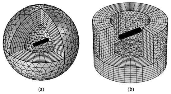
Figure 3.
The sound radiation model for a structure: (a) free field and (b) half-space.
The vibration of the structure should be acquired in advance as the input of the prediction methods. Meanwhile, the vibration information of the structure could be regarded as the references of vibration reconstruction in VR-ESM. However, it is often difficult to obtain the vibration of a structure in the fluid, especially when reflection boundaries exist to reinforce the acoustic–solid coupling effect. Luckily, in COMSOL, it is convenient to solve the problem as the FEM algorithm is the basic of the software. Especially, at low frequencies, the vibration could be obtained via FEM with a tiny computational cost.
To acquire the vibration of the structure when the parameters of the fluid, the structure, and the excitations are given out in advance, the structural FEM equation and the acoustical FEM equation should be solved simultaneously. The coupling relationship between the two equations is expressed by the continuity of the structural normal velocity and the particle velocity of the fluid on the structural surface. Then, the structural vibration and the sound field could be computed easily in the solution domain as all the computational processes are completed inside the software. Moreover, the structural modal analysis could also be carried out with FEM. The development of the method is introduced in detail in the study [15].
As FEM–BEM is a mature algorithm for sound prediction, the prediction results of FEM–BEM are considered as the references of the other prediction methods in the following extent. The computational process of FEM relies on the meshing of structure and the fluid domain, making it computational costly to complete the sound prediction at a long distance with FEM. Therefore, scholars take advantage of BEM in saving computation to complete the sound prediction at arbitrary positions in the sound field [7]. BEM is based on the Helmholtz integral equation as Equation (27):
where is a coefficient that is related to the position with the sound field point . When is outside the structure, . represents the integral points on the structural surface and is the normal velocity at [3]. It could be found that and has been obtained in the process of FEM. Thus, the computation of BEM could be completed. From the above introductions, FEM could be combined with BEM to utilize the advantages of the two methods. As the acoustical input of the other prediction methods such as ESM, CMESM, and VR-ESM is the normal velocities on the structure, the operation is the same as the abovementioned introduction.
3.1. The Measurement Point Arrangement Determined by SVM
When designing the measurement points on the surface of the structure, the measurement points are usually distributed on the structural surface uniformly in conventional strategies. In the theory of BEM, the interval between two adjacent measurement points should not be larger than one-sixth of the wavelength [16]. However, the criterion is not universal, especially when the frequency is quite low. Because the sound radiation at low frequencies is more of a concern in this paper, the theory of SVM should be adopted to be the guidance. In the work [7], Wang pointed out that the vibration sampling interval is closely linked with the structural wavenumber, orientations of the observation points, and the target prediction error. Take a cylindrical shell with finite length as the example, the numbers of vibration sampling points along the axial direction and the circumferential direction obey different rules. It could be mainly summed up that, for most observation points in the sound field, no matter whether along the axial direction or the circumferential direction, the vibration sampling points should at least satisfy the Nyquist sampling law, and the number of measurement points should not be less than twice the modal order in this direction. Especially in the axial direction, the measurement points are usually denser. The number of axial measurement points is nearly directly proportional to the axial modal order, . is the axial measurement points and is the axial modal order. is a coefficient related to the level of intended prediction error and is given in Table 1.

Table 1.
Values of with respect to the intended prediction errors.
According to the study of Wu [37], the value of is usually chosen to be 3~4 in engineering to ensure the accuracy of sound prediction.
Suppose that the structure is a cylindrical shell with fixed ends. The length of the cylindrical shell is , the radius is , and the thickness is . The material of the shell is steel, with a density of , Young’s modulus of , and Poisson’s ratio of 0.3. The detail of structural modes could be calculated by COMSOL Multiphysics. When at different frequencies, the modal response could be extremely different. Even with the same excitation frequency, the existence of the reflection boundary could change the added mass of water to the structure. Thus, the natural frequency of the structure for every structural mode may change, which means that the modal response could change. Some modes are given out in Table 2. In the pictures, a dark color corresponds to a large displacement. In the study [17], Zhang pointed out that the low-order modes have an obvious characteristic of overall vibration in a large area, which leads to their higher sound radiation efficiency. However, in Table 2, it could be found that, at higher-order modes, the radiation efficiency could still not be neglected as the large displacement areas occupy most of the radiation surface. According to the theory of modal superposition, the displacement of the shell could be expressed in the form of modal superposition. In order to complete the sound prediction accurately, all the vibration modes should be collected with the measurement system. Therefore, the mode with the highest order determines the criterion of vibration sampling, which means that the intervals between two adjacent measurement points depend on the structural wavenumbers along the certain directions.
Table 2.
Some low-order modes and modal natural frequencies in different acoustical environments.
In Table 2, is the submerged depth of the structure. The modal natural frequency is and the order of structural mode is . It could be seen that, with the existence of reflection boundary, the modal natural frequency of every mode could change. When the structure is quite close to the boundary that is considered to be ‘soft’, the modal natural frequency for the certain mode increases because the added mass of water decreases. Conversely, the modal natural frequency is close to the free-field-case when the structure is not close to the boundary. For example, when and the excitation frequency is 31.4 Hz, mode is not included. However, in the free field, mode should be included in the total modes. In other words, when in the half-space and the submerged depth is quite small, the variations of SVM details make it necessary to adjust the measurement point arrangement to meet the practical requirements.
The sound prediction is accomplished with ESM. The quantities of equivalent sources and the measurement points are determined with the rule presented in the study [13]. The equivalent source surface and the structure are conformal and the Recess ratio of the equivalent source is chosen to be 0.6~0.8 to avoid the ill-condition problem of the dipole matrix [9]. The coordinate system and the measurement points on the structure are shown in Figure 4.
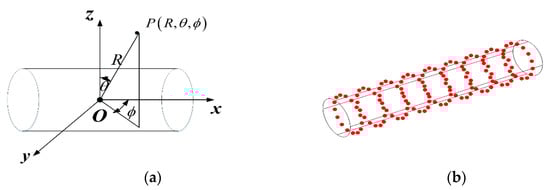
Figure 4.
(a) The coordinate system for the structure; (b) the measurement points on the structural surface.
Define as the excitation frequency. For example, when , if the structure is in free field, the highest order for the axial mode is 6, while it is 7 for the circumferential mode. However, when , the highest order for both the axial mode and the circumferential mode is 6. In other words, with the effect of reflection boundary, the highest circumferential mode changes. According to the theory of SVM, the vibration measurement along the circumferential direction should change with the modal variation.
To verify the theory of SVM, a prediction plane composed of observation points is set. The coordinates of the observation points are defined as follows: , , and (the interval between two adjacent points is 0.2 m). In the predictions of FEM–BEM, the measurement points are sufficiently dense (axial: 80; circumferential: 80) to ensure the accuracy of sound prediction. In order to quantitively evaluate the performance of the prediction methods, the prediction error of sound pressure amplitude is defined as , the prediction error of sound pressure phase is defined as , and are prediction results of sound pressure amplitude and phase, and and are the references of sound pressure amplitude and phase computed by FEM–BEM.
The prediction errors by ESM with sparse measurement points are shown in Figure 5 when the structure is in the free field. The number of measurement points is 270 (axial: 18; circumferential: 15), which has been proven to not be able to be reduced in either direction. The shell is excited with a point force of 50 N, which is located at (0,1,0) in Cartesian coordinates. Random noise with a signal–noise ratio (SNR) of 30 dB is added to the measured normal velocity to simulate the actual measurement. The medium is homogenous, with the density of and sound speed of .
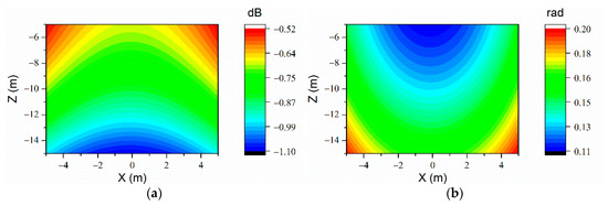
Figure 5.
The sound prediction errors of ESM on the prediction plane in the free field at the frequency of 71 Hz (270uniform arranged measurement points determined by SVM). (a) and (b) .
It could be seen in Figure 5 that, with the measurement points determined by SVM, using ESM, the prediction results could still be precise as the error of sound pressure level is always lower than 2 dB, while the error of sound pressure phase is always lower than . Prediction errors with the levels are quite low such that they could meet the engineering requests.
When the reflection boundary exists, the number of measurement points turns out to be 234 (axial: 18; circumferential: 13). The prediction results are shown in Figure 6. It could be seen that, with a tiny amount of measurement points, the sound prediction result in the half-space could also be accurate enough on the whole prediction plane. When the reflection boundary exists, the quantity of measurement points may change with the modal variation.
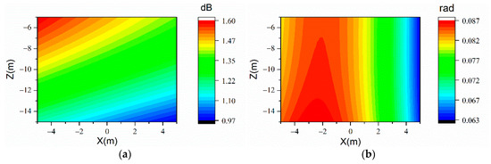
Figure 6.
The sound prediction errors of ESM on the prediction plane when at the frequency of 71 Hz (234 uniform arranged measurement points determined by SVM). (a) and (b) .
Thus, it could be seen that, if the detail of vibration modes could be obtained in advance, SVM could be an effective guidance to the design of the measurement system. The above simulations confirmed the possibility of sound prediction with a small-scale measurement system. However, it is difficult to acquire the exact detail of SVM in engineering via vibration measurement. Instead, the vibration modes could only be analyzed with numerical methods. Thus, it is often computationally costly to design the measurement system. Moreover, when the size of the structure is quite large or the excitation is complex, the details of structural vibration could be very complex, which means that an enormous quantity of measurement points are in need according to the theory of SVM [7]. Therefore, the method based on SVM could hardly be regarded as the optimal strategy of the measurement point arrangement.
3.2. The Sparse Measurement Point Arrangement Based on the Theory of ARM
A. The Results of CMESM
To illustrate the good convergence of ARM with the increase of order, the attenuation curves of ARM eigenvalues with the increase of the ARM order at different excitation frequencies are shown in Figure 7a. According to Section 2.3, a set of orthogonal basis is presented to give another expression of the equivalent source strengths. To verify that CMESM could enhance the sparsity of the equivalent source strengths, the normalized modal expansion coefficients with CMESM and ESM are shown in Figure 7b. In the simulation, the quantity of equivalent sources is 168. Meanwhile, 135 measurement points are uniformly distributed on the surface of the cylindrical shell in Section 3.1 (axial: 9; circumferential: 15).
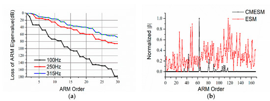
Figure 7.
(a). Attenuation curves of ARM eigenvalues with the increase of the ARM order at different frequencies (unit: dB); (b) comparison of the normalized modal expansion coefficient sparsity between ESM and CMESM at the frequency of 100 Hz.
It could be seen in Figure 7a that the eigenvalues of ARMs decrease rapidly with the increase of ARM order. At the higher excitation frequency, the eigenvalues decrease more slowly. Still, the big losses of ARM eigenvalues indicate that only the first few orders of ARMs contribute to the sound field. In Figure 7b, it could be seen that, compared with ESM, the modal expansion coefficients for CMESM are much sparser. Thus, though equivalent source strengths for the structure may not be sparse enough, the modal expansion coefficients of ARMs could be quite sparse, which allows sparse vibration measurement. Before the sound prediction, the sparsity of the modal expansion coefficient vector should be guaranteed to keep the prediction result accurate.
Repeat the simulations in Section 3.1. The quantity of measurement points is reduced to 90 (axial: 6, circumferential: 15), which is far less than in Section 3.1. Define as the condition number of the sensing matrix, . The variation of versus the ARM order is shown in Figure 8. The prediction results are shown in Figure 9. Several values of at different orders are given in Table 3. According to the study of Li [30], it is essential to reduce the value of for computing ARMs more stably. Otherwise, the poorly conditioned sensing matrix will give rise to large prediction errors.
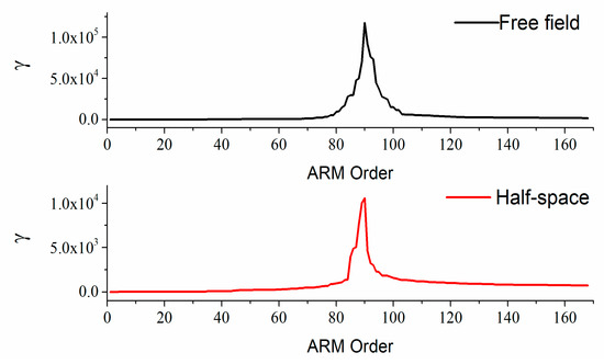
Figure 8.
The variation of with the increase of ARM order when 90 uniform-arranged measurement points are used.
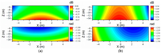
Figure 9.
The sound prediction errors of CMESM on the prediction plane when 90 uniformly arranged measurement points are used at the frequency of 71 Hz. (a) Free field (, upper:; lower: ) and (b) (, upper:; lower: ).
Table 3.
Different acoustic radiation mode (ARM) truncation numbers in compressed modal equivalent source method (CMESM) for 90 measurement points.
In Figure 8 and Table 3, it could be seen that, with the increase of ARM order, increases rapidly. After reaching the maximum, begins to decrease. Meanwhile, the values of at high orders are still much higher than those for the lower orders. Therefore, it is not appropriate to fix the ARM truncation number as high as possible. If is extravagantly large, the sensing matrix needs regularization [32]. In addition, it is not difficult to find that reaches the maximum when .
As shown in Figure 9, it could be seen that, with uniform measurement point arrangement, the sound prediction results are not satisfying. Though the prediction error of sound pressure amplitude could be quite low after adjusting , the prediction error of the sound pressure phase could still be awful as the ill-condition problem of sensing matrices may be inevitable when the measurement points are uniformly arranged and excessively sparse. Though regularization methods are introduced to solve the ill-condition problem of the sensing matrices, the result of sound prediction is still limited. Meanwhile, when the value of is quite low, the solutions of may not exist as the solutions of underdetermined equations could hardly have extravagantly high accuracy. Increasing the value of could help in obtaining a solution of , but the accuracy of the ARMs could not be guaranteed.
The quality of the prediction could be improved via increasing the quantity of measurement points [31]. Therefore, increasing the measurement point quantity to 135, the variation of with the increase of ARM order is shown in Figure 10. Several values of at different orders are given in Table 4.
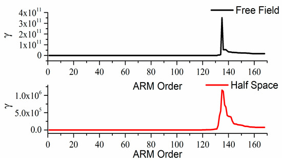
Figure 10.
The variation of with the increase of ARM order when 135 uniformly arranged measurement points are used.
Table 4.
Different ARM truncation numbers in CMESM for 135 measurement points.
Compared with Table 3, it could be found in Table 4 that, when the quantity of measurement points increases to 135, the values of could also be quite low at high orders, which is beneficial to find the balance between computation convergence and prediction robustness. Repeating the simulation in Section 3.1, the prediction errors are shown in Figure 11. It could be seen that, with more measurement points, the prediction results become much better because it is easy to obtain optimal solutions of that satisfy the sparsity and the penalty terms. Meanwhile, it is not necessary to change the quantity of measurement points when the reflection boundary exists, which breaks through the limitation of the SVM.
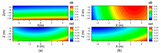
Figure 11.
The sound prediction errors of CMESM on the prediction plane when 135 uniformly arranged measurement points are used at the frequency of 71 Hz. (a) Free field (, upper:; lower: ) and (b) (, upper:; lower: ).
However, the expansion of the measurement system scale will definitely increase the engineering cost. Bi and Li indicated that, with a fixed scale of the measurement system, a non-uniform system could have better performance in sound prediction than a uniform system [28,30]. However, the optimization method was not introduced in those works. Therefore, the EFI could be applied for optimizing the measurement system. With the help of the EFI, the measurement points contributing most to the ARMs are picked out from the candidate set.
B. The Results of VR-ESM
Repeat the simulations in Section 3.1. The quantity of measurement points is fixed at 90. The optimal values of are 42 and 35, which are determined by the method in Section 2.3. Define as the condition number of, . The variation of versus the ARM order is shown in Figure 12a. The reconstruction errors versus the ARM order are shown in Figure 12b. A total of 32 measurement points are selected as test points, whose arrangement is shown in Figure 12c. For observing the measurement point arrangement conveniently, the shell is spread into the planar form along the circumferential direction as Figure 12c.
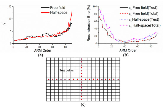
Figure 12.
(a) The variation of with the increase of ARM order, (b) the variation of reconstruction error versus the ARM order (, ), and (c) the arrangement of test points.
From Figure 12a, it could be seen that, although increases with the increase of ARM order, the value of is quite low. Thus, the reconstruction of vibration could be quite robust. As shown in Figure 12b, the tendencies of versus the ARM order are similar for test points and total points, which manifests the efficiency of the reconstruction method. It could be seen that, with the increase of ARM order, decreases at the first orders to reach the minimum, which means that the computations reach the convergence when orders are used. However, when the ARM order continues to increase, begins to increase because also increases, which means that the prediction errors caused by the noise could be reinforced. Thus, it is still necessary to select the optimal to keep the prediction accurate. The prediction results and the measurement point arrangements are shown in Figure 13 and Figure 14. The truncation numbers of ARMs are selected to be 42 and 35 for the free field and half-space, respectively.
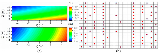
Figure 13.
The sound prediction errors of VR-ESM on the prediction plane in the free field at the frequency of 71 Hz, . (a) Upper: ; lower: . (b) The arrangement of measurement points (90 points optimized with EFI).
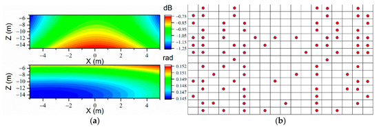
Figure 14.
The sound prediction errors of VR-ESM on the prediction plane when at the frequency of 71 Hz, . (a) Upper: ; lower: . (b) The arrangement of measurement points (90 points optimized with EFI).
It could be seen that the prediction results are enough accurate with VR-ESM though the measurement points are quite sparse, which verifies the efficiency of VR-ESM. When the quantity of measurement points is fixed, compared with the uniform measurement point arrangement in CMESM, more accurate prediction results could be obtained with the VR-ESM when the measurement point arrangement is optimized with the EFI, as the independence among the measurement points is reinforced by minimizing the condition number of the sensing matrix.
To verify the necessity of the optimization process with EFI, the prediction results of VR-ESM with uniform measurement points (axial: 6; circumferential: 15) are shown in Figure 15. The optimal are determined by minimizing .
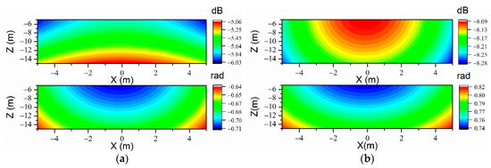
Figure 15.
The sound prediction errors of VR-ESM on the prediction plane at the frequency of 71 Hz when 90 uniformly arranged measurement points are used. (a) Free field (upper: ; lower: , ); (b) (upper: ; lower: , ).
It could be seen that, with uniform and sparse measurement points, the prediction results are not accurate. The phenomenon could be explained by the ill-condition problem of the sensing matrices. The condition numbers of the sensing matrices are given in Table 5. It could be seen that the ill-condition problem of the sensing matrices could be severe without the optimization of the EFI. Thus, though the values of are determined after minimizing the reconstruction errors, the prediction results could still be unsatisfying. On the contrary, after the optimization of the EFI, the ill-condition problem could be improved. Therefore, it is necessary to optimize the measurement point arrangement with EFI to improve the prediction accuracy.
Table 5.
Different values of in vibration reconstruction equivalent source method (VR-ESM) with 90 measurement points. EFI, efficient independence.
4. Discussion
According to the simulations in Section 3.2, the effect of EFI on improving the prediction accuracy of VR-ESM is obvious. Meanwhile, whether the optimal measurement system obtained with the EFI is appropriate for the CMESM is of interest to be discussed. In the following simulation, the measurement systems are the same as Figure 13b and Figure 14b, the sound predictions are completed by CMESM, and other simulation parameters remain unchanged. The results are shown in Figure 16.
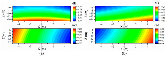
Figure 16.
The sound prediction errors of CMESM on the prediction plane at the frequency of 71 Hz when 90 measurement points are used (optimized with EFI). (a) Free field (upper: ; lower: , ); (b) (upper: ; lower: , ).
From Figure 16, it is interesting to find that, with the optimal measurement system obtained with the EFI, the prediction results of CMESM are also acceptable. It could also be explained by the ill-condition problem of the sensing matrices. The values of with different types of measurement systems are given in Table 6.
Table 6.
Different values of in CMESM with 90 measurement points.
Generally, for structures with regular shapes, the velocity ARMs usually have good spatial symmetry, which will reinforce the ill-condition problem of sensing matrices for uniform measurement point arrangement [30]. Though the optimal measurement system obtained with the VR-ESM and EFI is not necessarily optimal for the CMESM, the ill-condition problem of sensing matrices could also be limited efficiently, which allows more accurate and robust solutions of . Thus, the quality of sound predictions could also be improved.
From the above analyses, the sound prediction based on sparse vibration measurement has been proven to be efficient. However, there still exist some factors that could affect the prediction, such as the submerged depth and the signal–noise ratio. Meanwhile, whether the method could be applied for other compute frequencies has not been discussed yet. Thus, the above factors will be discussed in the following content. To save space, when evaluating the prediction accuracy, define the average prediction errors of sound pressure amplitude and phase as follows: , , where is the quantity of field points on the plane.
A. Sound Prediction with Different Frequencies
Repeat the simulation in Section 3.1, , and select 21 frequency points ranging from 200 Hz to 500 Hz. The measurement systems are optimized with the EFI and the quantity of measurement points is 90. The prediction errors versus frequency are shown in Figure 17.
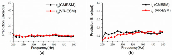
Figure 17.
Prediction errors of sound pressure and phase at different frequencies (). (a) and (b) .
From Figure 17, it could be seen that, at different frequencies, both the CMESM and the VR-ESM could be well applied for the sound prediction. If the measurement system is designed with the SVM, the scale of the measurement system will definitely change with the variation of the SVM. On the contrary, the quantity of measurement points could remain invariant in a particular frequency band, which highlights the advantage of the methods based on the theory of the ARM.
B. The Influence of SNR
Furthermore, the influence of SNR on the prediction results is also investigated. Figure 18 shows the prediction errors of the two methods based on the ARM with the variation of SNR at 300 Hz when 90 measurement points are used. The submerged depth is 0.2 m and the measurement system is optimized with the EFI.
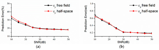
Figure 18.
Prediction errors with the variation of the signal–noise ratio (SNR) (, 90 measurement points optimized with EFI). (a) and (b).
It could be seen that the prediction qualities of VR-ESM and CMESM become better with the increase of SNR. When the SNR is high enough, the prediction errors tend to be invariant. As the SNR is usually high enough in the real measurement of normal velocity, the method could be efficient in engineering.
C. The Influence of Submerged Depth
In the above content, the submerged depth of the source is quite small, such that the influence of reflection sounds on the structural vibration could not be neglected. Thus, when decomposing the power resistance matrix , the half-space Green function has to be used in the construction of dipole matrix to eliminate the disturbance of reflection sounds, which leads to extra computation. However, with the increase of submerged depth, the influence of is weakened. When could be neglected, the dipole matrix is approximated to and almost half of the computation is saved. To verify the conclusion, a simulation is proposed when . Define the prediction where is the dipole matrix as the SFS case and the prediction where is the dipole matrix as the Quick case. The prediction errors with the variations of are shown in Figure 19, where is the radius of the structure.
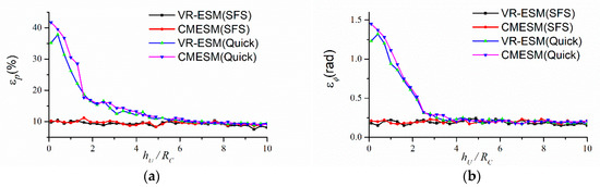
Figure 19.
Prediction errors at different submerged depths in the SFS case and Quick case when 90 measurement points are used (, ). (a) and (b) .
It could be seen that, in the SFS case, the prediction result could be accurate at an arbitrary submerged depth. However, in the Quick case, the prediction errors are quite large at a small submerged depth because the ARMs could not be calculated accurately when the influence of could not be neglected. When the submerged depth increases, the prediction results become more accurate. In the above simulation, when exceeds 5, the prediction results in the Quick case could also be acceptable. In fact, for a real elastic structure, the influence of reflection sounds on the structural vibration depends on many factors such as shape, size, thickness, material, and frequency. It is a complex problem that involves fluid–solid coupling, scattering, and sound propagation. Because of the limited space, only the influence of submerged depth is discussed in this paper. Because all the ARMs derive from the equivalent sources inside the structure, suppose that the maximum dimension of the structure is , the mean distance between and Ω is usually less than . In contrast, the mean distance between and is more than . According to the attenuation rule of monopole and Equation (11), it is easy to conclude that is an order of magnitude less than when is satisfied. In other words, when the submerged depth is large enough, could be used as the dipole matrix instead of and the Quick case goes into effect. There are two advantages of using the Quick case when the application condition is satisfied. Firstly, it is not necessary to compute and almost half of the computation is reduced, which is beneficial for fast prediction. Secondly, the stability of the prediction is reinforced without the participant of , as the condition number of is usually large such that the regularization process is necessary.
5. Conclusions and Prospects
In this paper, two methods of predicting the sound field of submerged structure with sparse measurement points are proposed. It has been proven that the method could be applied for a structure located in the half-space. With some simulations, several significant conclusions could be obtained as below:
- (a)
- When arranging measurement points on the surface of the source, the traditional method based on the SVM should at least obey the Nyquist sampling rule. In other words, the quantity of measurement points mainly depends on the highest order of the vibration modes in every direction. When the reflection boundary exists and is quite close to the structure, the details of SVM may change and the measurement point arrangement should change at some special frequencies. However, to compute the exact detail of SVM is computationally costly, especially when the size of the structure is large, the shape of the structure is irregular, the coupling effect of reflection sounds could not be neglected, and so on. Therefore, the measurement point arrangement based on SVM could hardly be regarded as the optimal arrangement.
- (b)
- With the theory of ARM, the quantity of measurement points could be much smaller than for the SVM, as the sound field could be expressed well with only few ARMs. However, the ill-condition problem of the sensing matrices affects the prediction accuracy. Though arranging measurement points uniformly is easy and convenient in engineering, it could hardly be regarded as the optimal arrangement as the ill-condition problem could be severe to reinforce prediction errors. Adding more points to the measurement set could improve the prediction accuracy as well as increase the computation. Therefore, with a fixed quantity of measurement points, the arrangement should be optimized to avoid the ill-condition problem of the sensing matrices. With the optimization of the EFI, the condition number of the sensing matrix is limited and the stability and accuracy of prediction could be guaranteed.
- (c)
- Some factors that may affect the prediction accuracy are also analyzed in this paper, such as the truncation number of ARMs , SNR, computer frequency , and the submerged depth . Some conclusions could be given as below:
- The proposed method could be well applied for different frequencies. However, the arrangement of measurement points could have a significant influence on the prediction result. It is still necessary to manage the arrangement with EFI to reduce the prediction errors.
- The prediction accuracy could be satisfying when the SNR is high enough.
- When the ARM truncation number is either excessively small or excessively big, the prediction errors are remarkable. Thus, the optimal truncation number of ARMs should be selected appropriately according to the prediction errors at the test points.
- When the submerged depth is quite small such that the structural vibration is obviously affected by the reflection sounds, it is necessary to use SFS to maintain the accuracy of the prediction result. However, when the submerged depth is large enough, the dipole matrix for the free field could be used to construct the ARMs and the prediction results could also be accurate. The benefit is that not only the computation is reduced, the stability of the prediction is also reinforced.
Though there was no experimental result in this paper because it is difficult for the researchers to acquire satisfying experimental conditions in the laboratory, the method of carrying out experimental research could still be designed as in the following steps:
- Choose an appropriate experimental environment. To simulate a structure with finite submerged depth, the experiment should be carried out in open water to avoid the effect of reflection sounds from the horizontal direction. Meanwhile, the depth of the water should be enough large that the reflection sounds from the bottom could be neglected.
- Design the distribution of equivalent sources according to the shape of the structure and calculate the dipole matrices and , and the power resistance matrix .
- Optimize the measurement point arrangement in advance with EFI and dispose of vibration transducers at these points.
- Construct ARMs with VR-ESM and CMESM and complete the sound prediction. To verify the effectiveness of the methods, the measurement results in the sound field could be regarded as the references.
The methods proposed in this paper could help in optimizing measurement systems for submerged vehicles with a large size, especially in non-free fields. On the premise of ensuring the prediction accuracy, it saves engineering cost compared with the traditional method based on the SVM. Meanwhile, the combinations with the SFS broaden the applications of the methods. However, there still exist some complicated conditions such as waveguide and irregular structural shape that are not discussed in this paper because of space constraints. In further studies, we anticipate discussions about more complicated conditions to better meet engineering requirements.
Author Contributions
Conceptualization, W.W.; Funding acquisition, D.Y. and J.S.; Investigation, D.Y. and J.S.; Methodology, W.W.; Software, W.W.; Supervision, D.Y. and J.S.; Visualization, W.W.; Writing—original draft, W.W.; Writing—review & editing, J.S. All authors have read and agreed to the published version of the manuscript.
Funding
This research was funded by the National Nature Science Foundation of China (grant.No.11674074).
Conflicts of Interest
The authors declare no conflict of interest.
References
- Chen, H. Research on Prediction of Sound Radiated by Elastic Structure in Underwater Bounded Space. Ph.D. Thesis, Harbin Engineering University, Harbin, China, 2013. [Google Scholar]
- Qian, Z.; Shang, D.; Sun, Q.; He, Y.; Zhai, J. Acoustic radiation from a cylinder in shallow water by finite element-parabolic equation method. Acta Phys. Sin. 2019, 68, 139–152. [Google Scholar]
- Miao, Y.; Li, T.; Zhu, X.; Wang, P.; Zhang, G. Research on the acoustical radiation characteristics of cylindrical shells in a shallow sea. J. Harbin Eng. Univ. 2017, 38, 719–726. [Google Scholar]
- Guo, W.; Li, T.; Zhu, X.; Miao, Y.; Zhang, G. Vibration and acoustic radiation of a finite cylindrical shell submerged at finite depth from the free surface. J. Sound Vib. 2017, 393, 338–352. [Google Scholar] [CrossRef]
- Von Estorff, O. Acoustic investigation of objects in shallow water using FEM and BEM. J. Acoust. Soc. Am. 1999, 105, 1165. [Google Scholar] [CrossRef]
- Yang, D.; Wang, W.; Shi, J.; Zhang, Y. Low-frequency vector sound field modeling and simulation analysis of a cylindrical shell with finite submerged depth. J. Harbin Eng. Univ. 2020, 41, 166–174. [Google Scholar]
- Wang, B. Research on Prediction of Noise Radiated by Large Underwater Structures via Surface Vibration Monitoring. Ph.D. Thesis, Shanghai JiaoTong University, Shanghai, China, 2008. [Google Scholar]
- Koopmann, G.H.; Song, L.; Fahnline, J.B. A method for computing acoustic fields based on the principle of wave superposition. J. Acoust. Soc. Am. 1989, 86, 2433–2438. [Google Scholar] [CrossRef]
- Li, J.; Chen, J.; Yang, C.; Jia, W. Analysis of the impact factors on the accuracy of sound field reconstruction based on wave superposition. Acta Phys. Sin. 2008, 57, 4258–4264. [Google Scholar]
- Huang, H.; Zou, M.S.; Jiang, L.W. Study on the integrated calculation method of fluid-structure interaction vibration, acoustic radiation, and propagation from an elastic spherical shell in ocean acoustic environments. Ocean Eng. 2019, 177, 29–39. [Google Scholar] [CrossRef]
- Xiang, Y.; Huang, Y. Wave Superposition method based on virtual source boundary with complex radius vector for solving acoustic radiation problems. Acta Mech. Solid Sin. 2004, 25, 35–41. [Google Scholar]
- Gao, Y.; Cheng, H.; Chen, J. Acoustic radiation sensitivity analysis of semi-free field. Trans. Chin. Soc. Agric. Mach. 2008, 39, 179–183. [Google Scholar]
- Wang, Y. Theoretical and Experimental Research of Underwater Noise Reduction Prediction Based on Wave Superposition Method. Ph.D. Thesis, Harbin Engineering University, Harbin, China, 2013. [Google Scholar]
- Huang, H.; Zou, M.; Jiang, L. Computing method of sound radiation of target in ocean acoustic environment. Acta Acust. 2019, 44, 79–87. [Google Scholar]
- Shang, D.; Qian, Z.; He, Y.; Xiao, Y. Sound radiation of cylinder in shallow water investigated by combined wave superposition method. Acta Phys. Sin. 2018, 67, 084301. [Google Scholar]
- Tao, J.; Ge, H.; Qiu, X. A new rule of vibration sampling for predicting acoustical radiation from rectangular plates. Appl. Acoust. 2006, 67, 756–770. [Google Scholar] [CrossRef]
- Zhang, C.; Li, S.; Shang, D.; Han, Y.; Shang, Y. Prediction of sound radiation from submerged cylindrical shell based on dominant modes. Appl. Sci. 2020, 10, 3073. [Google Scholar] [CrossRef]
- Photiadis, D.M. The relationship of singular value decomposition to wave-vector filtering in sound radiation problems. J. Acoust. Soc. Am. 1990, 88, 1152–1159. [Google Scholar] [CrossRef]
- Borgiotti, G.V. The power radiated by a vibrating body in an acoustic fluid and its determination from boundary measurements. J. Acoust. Soc. Am. 1990, 88, 1884–1893. [Google Scholar] [CrossRef]
- Elliott, S.J.; Johnson, M.E. Radiation modes and the active control of sound power. J. Acoust. Soc. Am. 1993, 94, 2194–2204. [Google Scholar] [CrossRef]
- Cunefare, K.A.; Currey, M.N. On the exterior acoustic radiation modes of structures. J. Acoust. Soc. Am. 1994, 96, 2302–2312. [Google Scholar] [CrossRef]
- Bouchet, L.B.; Loyau, T.; Hamzaoui, N.; Boission, C. Calculation of acoustic radiation using equivalent sphere methods. J. Acoust. Soc. Am. 2000, 107, 2387–2397. [Google Scholar] [CrossRef]
- Sarkissian, A. Acoustic radiation from finite structures. J. Acoust. Soc. Am. 1991, 90, 574–578. [Google Scholar] [CrossRef]
- Mao, Q.; Jiang, Z. Research active structural acoustic control by radiation modes. Acta Acust. 2001, 26, 277–281. [Google Scholar]
- Nie, Y.; Zhu, H.; Mao, R. Mode analysis method for structure’s sound radiation analysis based on source intensity acoustic radiation modes. Noise Vib. Control 2014, 34, 1–5. [Google Scholar]
- Zhan, G.; Mao, R. A new acoustic radiation mode calculation method based on wave superposition method. J. Naval Univ. Eng. 2016, 28, 4–8. [Google Scholar]
- Efren, F.G.; Angeliki, X.G. A sparse equivalent source method for near-field acoustic holography. J. Acoust. Soc. Am. 2017, 141, 532–542. [Google Scholar]
- Bi, C.; Liu, Y.; Xu, L.; Zhang, Y. Sound field reconstruction using compressed modal equivalent point source method. J. Acoust. Soc. Am. 2017, 141, 73–79. [Google Scholar] [CrossRef] [PubMed]
- Jᴓrgen, H. A comparison of compressive equivalent source methods for distributed sources. J. Acoust. Soc. Am. 2020, 147, 2211–2221. [Google Scholar]
- Li, X.; Zhao, D. Study on influence of measurement point distribution on reconstruction of acoustic fields based on acoustic radiation mode. Chin. Intern. Combust. Eng. Eng. 2010, 31, 69–73. [Google Scholar]
- Su, J.; Zhu, H.; Mao, R.; Guo, L.; Su, C. Optimization of measurement points in reconstruction of acoustic field based on acoustic radiation modes. J. Vib. Shock 2017, 36, 145–150. [Google Scholar]
- Mao, R.; Zhu, H. Structure normal velocity reconstruction with sparse measurement points. Chin. J. Acoust. 2018, 37, 60–68. [Google Scholar]
- Tian, K.; Mao, J.; Li, L.; Cui, Y.; Du, J. Direct sound field separation method based on single holographic layer particle velocity measurements. Noise Vib. Control 2019, 39, 27–31. [Google Scholar]
- Sarkissian, A. Method of superposition applied to patch near field acoustic holography. J. Acoust. Soc. Am. 2005, 118, 671–678. [Google Scholar] [CrossRef]
- Tikhonov, A.N.; Arsenin, V.Y. Solution of Ill-Posed Problems; Winston: Washington, DC, USA, 1977; pp. 55–60. [Google Scholar]
- Sun, C. Theoretical and Its Application Investigation on Near Field Acoustic Holography for Underwater Structures in Confined Space. Ph.D. Thesis, Harbin Engineering University, Harbin, China, 2013. [Google Scholar]
- Wu, H.; Zhang, Y.; Jiang, W. An interpolation method for the measured velocity and its application in the prediction of acoustic radiation of submerged cylindrical shell structures. Acta Acust. 2015, 40, 631–638. [Google Scholar]
- Liu, Y. Research on the Reconstruction and Separation of the Sound Field Radiated by the Sources with Arbitrary Shape Based on Sparse Sampling. Ph.D. Thesis, Hefei University of Technology, Hefei, China, 2019. [Google Scholar]
- Chardon, G.; Daudet, L.; Pillot, A.; Ollivier, F.; Bertin, N.; Gribonval, R. Near-field acoustic holography using sparse regularization and compressive sampling principles. J. Acoust. Soc. Am. 2012, 132, 1521–1534. [Google Scholar] [CrossRef] [PubMed]
- Grant, M.; Boyd, S. CVX: Matlab Software for Disciplined Convex Programming, Version 1.21. Available online: http://cvxr.com/cvx (accessed on 24 February 2011).


Publisher’s Note: MDPI stays neutral with regard to jurisdictional claims in published maps and institutional affiliations. |
© 2021 by the authors. Licensee MDPI, Basel, Switzerland. This article is an open access article distributed under the terms and conditions of the Creative Commons Attribution (CC BY) license (http://creativecommons.org/licenses/by/4.0/).