3D Gravity Inversion on Unstructured Grids


Abstract
:1. Introduction
2. Methods
2.1. Gravity Forward Modeling Based on Tetrahedral Grids
2.2. Fuzzy C-Means Clustering Inversion with Spatial Constraints
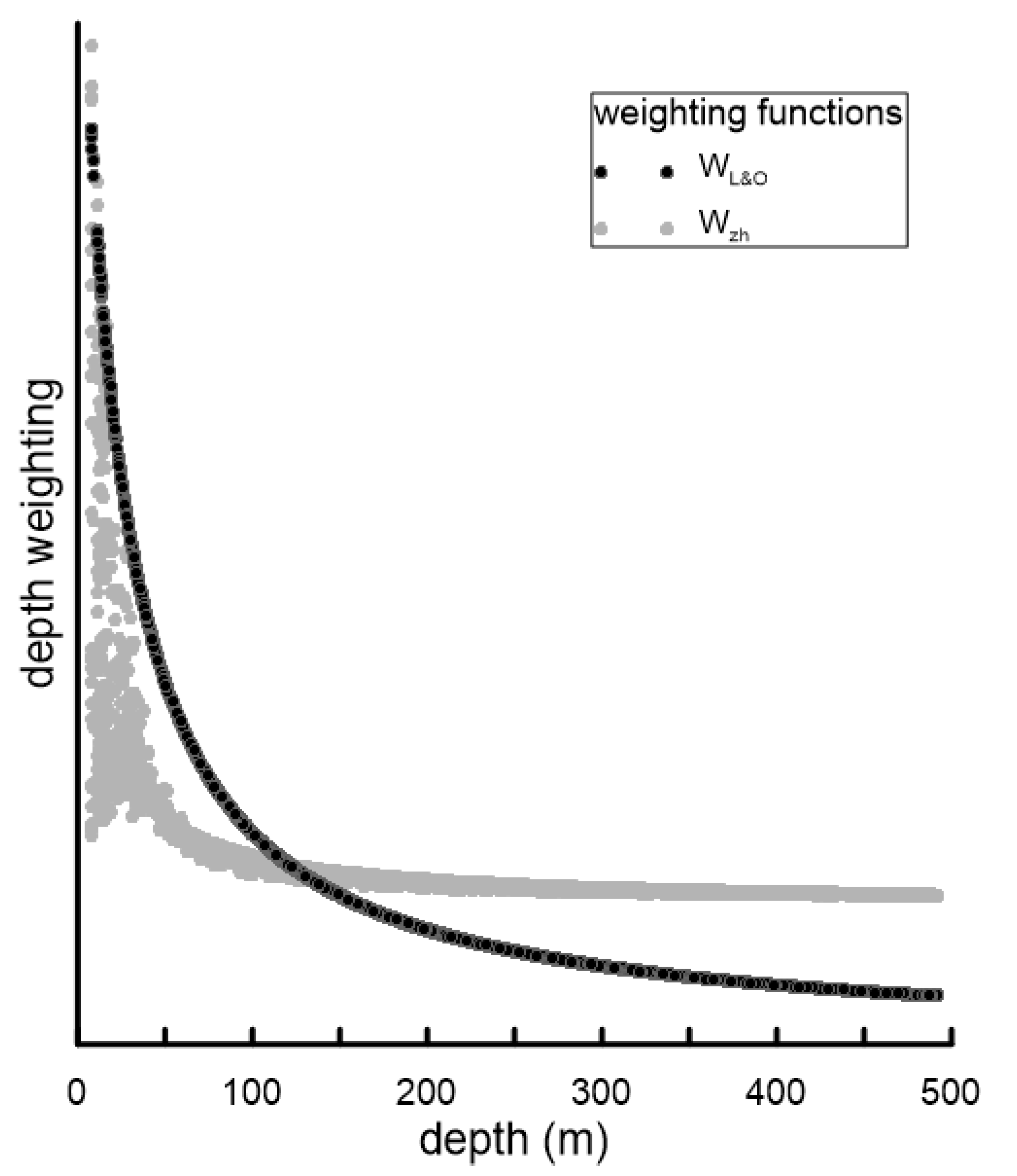
3. Analysis of Depth Weighting on Unstructured Grids
4. Results
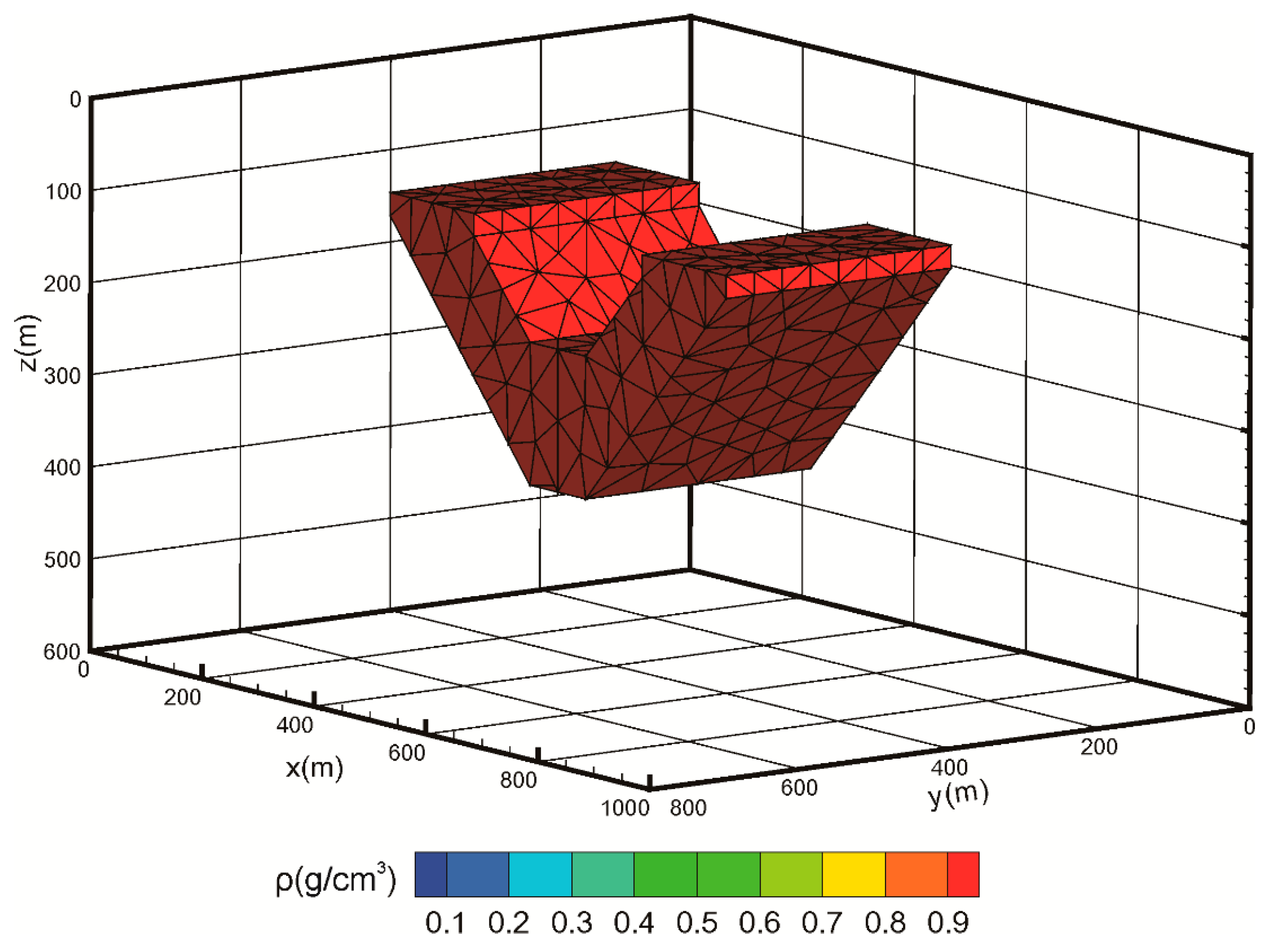
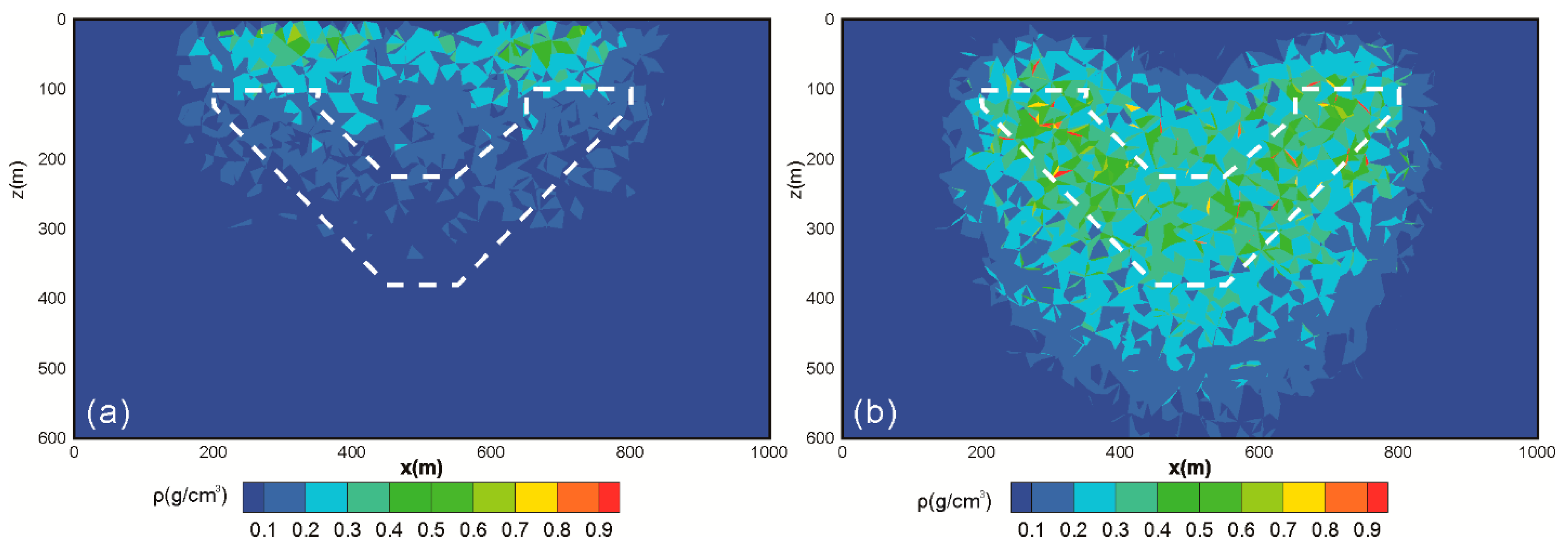
4.1. Inversions of Simulation Data
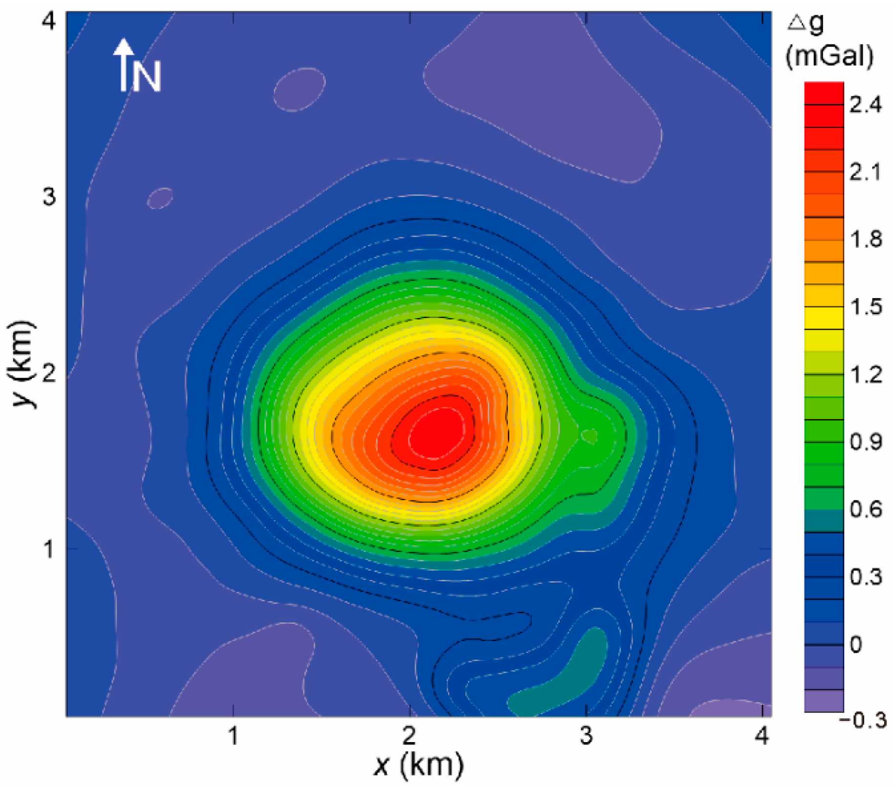
4.2. Field Data Inversion
5. Conclusions
Author Contributions
Funding
Institutional Review Board Statement
Informed Consent Statement
Data Availability Statement
Acknowledgments
Conflicts of Interest
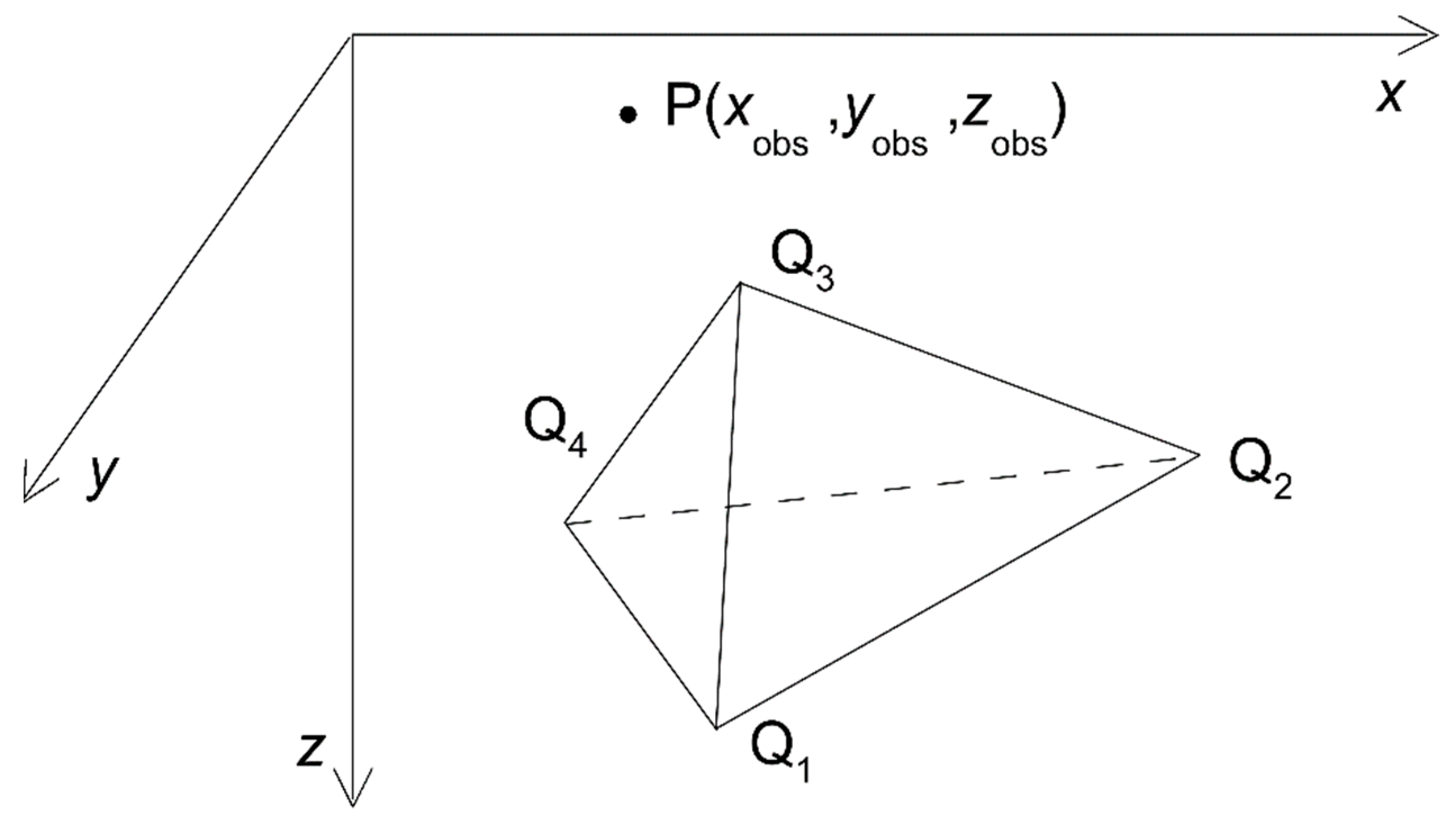
Appendix A
- Rotate counterclockwise the x- and y-axes around the z-axis in Figure A1a by the angle φ until the rotated x-axis is coincident with the direction of the outward normal onto the x-y-plane.
- Rotate counterclockwise the z- and x-axes around the y-axis by the angle ψ until the rotated z-axis is coincident with the outward normal direction of the triangle facet (Q1Q2Q3). With previous two rotations, we obtain the target coordinate system (X, Y, Z). Thus, the polygon is in the X-Y-plane, as shown in Figure A1b.
- Rotate counterclockwise the X-and Y-axes around the Z-axis by the angle θ until the rotated Y-axis is coincident with the direction of the outward normal on the edge Q1Q2 (as shown in Figure A1c).

References
- Talwani, M.; Ewing, M. Rapid computation of gravitational attraction of three-dimensional bodies of arbitrary shape. Geophysics 1960, 25, 203–225. [Google Scholar] [CrossRef]
- Talwani, M. Computation with the help of a digital computer of magnetic anomalies caused by bodies of arbitrary shape. Geophysics 1965, 30, 797–817. [Google Scholar] [CrossRef]
- Barnett, C.T. Theoretical modeling of the magnetic and gravitational fields of an arbitrarily shaped three-dimensional body. Geophysics 1976, 41, 1353–1364. [Google Scholar] [CrossRef]
- Okabe, M. Analytical expressions for gravity anomalies due to homogeneous polyhedral bodies and translations into magnetic anomalies. Geophysics 1979, 44, 730–741. [Google Scholar] [CrossRef]
- Zhang, J.; Wang, C.; Shi, Y.; Cai, Y.; Chi, W.; Dreger, W.; Cheng, W.; Yuan, Y. Three-dimensional crustal structure in central Taiwan from gravity inversion with a parallel genetic algorithm. Geophysics 2004, 69, 917–924. [Google Scholar] [CrossRef] [Green Version]
- Cai, Y.; Wang, C. Fast finite-element calculation of gravity anomaly in complex geological regions. Geophys. J. Int. 2005, 162, 696–708. [Google Scholar] [CrossRef] [Green Version]
- May, D.A.; Knepley, M.G. Optimal, scalable forward models for computing gravity anomalies. Geophys. J. Int. 2011, 187, 161–177. [Google Scholar] [CrossRef] [Green Version]
- Jahandari, H.; Farquharson, C.G. Forward modeling of gravity data using finite-volume and finite-element methods on unstructured grids. Geophysics 2013, 78, G69–G80. [Google Scholar] [CrossRef]
- Li, Y.; Oldenburg, D.W. 3-D inversion of gravity data. Geophysics 1998, 63, 109–119. [Google Scholar] [CrossRef]
- Boulanger, O.; Chouteau, M. Constraints in 3D gravity inversion. Geophys. Prospect. 2001, 49, 265–280. [Google Scholar] [CrossRef]
- Zhdanov, M.S.; Ellis, R.; Mukherjee, S. Three-dimensional regularized focusing inversion of gravity gradient tensor component data. Geophysics 2004, 69, 925–937. [Google Scholar] [CrossRef]
- Silva, D.F.J.; Barbosa, V.C.; Silva, J.B. 3D gravity inversion through an adaptive-learning procedure. Geophysics 2009, 7, I9–I21. [Google Scholar] [CrossRef]
- Tikhonov, A.N.; Arsenin, V.Y. Solution of Ill-Posed Problems; Wiley: New York, NY, USA, 1977; p. 258. [Google Scholar]
- Li, Y.; Oldenburg, D.W. 3-D inversion of magnetic data. Geophysics 1996, 61, 394–408. [Google Scholar] [CrossRef]
- Last, B.J.; Kubik, K. Compact gravity inversion. Geophysics 1983, 48, 713–721. [Google Scholar] [CrossRef]
- Portniaguine, O.; Zhdanov, M.S. 3-D magnetic inversion with data compression and image focusing. Geophysics 2002, 67, 1532–1541. [Google Scholar] [CrossRef] [Green Version]
- Lelièvre, P.G.; Farquharson, C.G.; Hurich, C.A. Joint inversion of seismic traveltimes and gravity data on unstructured grids with application to mineral exploration. Geophysics 2012, 77, K1–K15. [Google Scholar] [CrossRef]
- Sun, J.; Li, Y. Multidomain petrophysically constrained inversion and geology differentiation using guided fuzzy c-means clustering. Geophysics 2015, 80, ID1–ID18. [Google Scholar] [CrossRef]
- Sun, J.; Li, Y. joint inversion of multiple geophysical data using guided fuzzy c-means clustering. Geophysics 2016, 81, ID37–ID57. [Google Scholar] [CrossRef]
- Singh, A.; Sharma, S. Modified Zonal Cooperative Inversion of Gravity Data-a Case Study from Uranium Mineralization; SEG Technical Program Expanded Abstracts: Houston, TX, USA, 2017; pp. 1744–1749. [Google Scholar]
- Commer, M. Three-dimensional gravity modelling and focusing inversion using rectangular meshes. Geophys. Prospect. 2011, 59, 966–979. [Google Scholar] [CrossRef]
- Liu, Y.P.; Wang, Z.W.; Du, X.J.; Liu, J.H.; Xu, J.S. 3D constrained inversion of gravity data based on the Extrapolation Tikhonov regularization algorithm. Chin. J. Geophys. 2013, 56, 1650–1659. (In Chinese) [Google Scholar]
- Ren, Z.; Chen, C.; Pan, K.; Kalscheuer, T.; Maurer, H.; Tang, J. Gravity Anomalies of Arbitrary 3D Polyhedral Bodies with Horizontal and Vertical Mass Contrasts. Surv. Geophys. 2017, 38, 479–502. [Google Scholar] [CrossRef]
- Zhao, G.; Chen, B.; Chen, L.; Liu, J.; Ren, Z. High-accuracy 2D and 3D Fourier forward modeling of gravity field based on the Gauss-FFT method. J. Appl. Geophys. 2018, 150, 294–303. [Google Scholar] [CrossRef]
- Si, H. Tetgen: A Quality Tetrahedral Mesh Generator and a 3D Delaunay Triangulator. 2009. Available online: http://wias-berlin.de/software/index.jsp?id=TetGen&lang=1 (accessed on 25 September 2017).
- Hathaway, R.J.; Bezdek, J.C. Fuzzy c-means clustering of incomplete data: IEEE Transactions on Systems, Man, and Cybernetics, Part B. Cybernetics 2001, 31, 735–744. [Google Scholar] [PubMed] [Green Version]
- Fedi, M.; Rapolla, A. 3-D inversion of gravity and magnetic data with depth resolution. Geophysics 1999, 64, 452–460. [Google Scholar] [CrossRef]
- Li, Y.; Oldenburg, D.W. Joint inversion of surface and three-component borehole magnetic data. Geophysics 2000, 65, 540–552. [Google Scholar] [CrossRef]
- Dickinson, J.L.; Brewster, J.R.; Robinson, J.W.; Murphy, C.A. Imaging techniques for full tensor gravity gradiometry data. In Proceedings of the 11th SAGA Biennial Technical Meeting and Exhibition, Swaziland, South Africa, 16–18 September 2009. cp-241-00019. [Google Scholar]
- Coker, M.O.; Bhattacharya, J.P.; Marfurt, K.J. Fracture patterns within mudstones on the flanks o f a salt dome: Syneresis or slumping? Gulf Coast Assoc. Geol. Soc. 2007, 57, 125–137. [Google Scholar]
- Ennen, C. Mapping Gas-Charged Fault Blocks around the Vinton Salt Dome, Louisiana Using Gravity Gradiometry Data. Master’s Thesis, University of Houston, Houston, TX, USA, 2012. [Google Scholar]
- Salem, A.; Masterton, S.; Campbell, S.; Dickinson, J.D.; Murphy, C. Interpretation of tensor gravity data using an adaptive tilt angle method. Geophys. Prospect. 2013, 61, 1065–1076. [Google Scholar] [CrossRef]
- Thompson, S.A.; Eichelberger, O.H. Vinton salt dome, Calcasieu Parish, Louisiana. AAPG Bull. 1928, 12, 385–394. [Google Scholar]

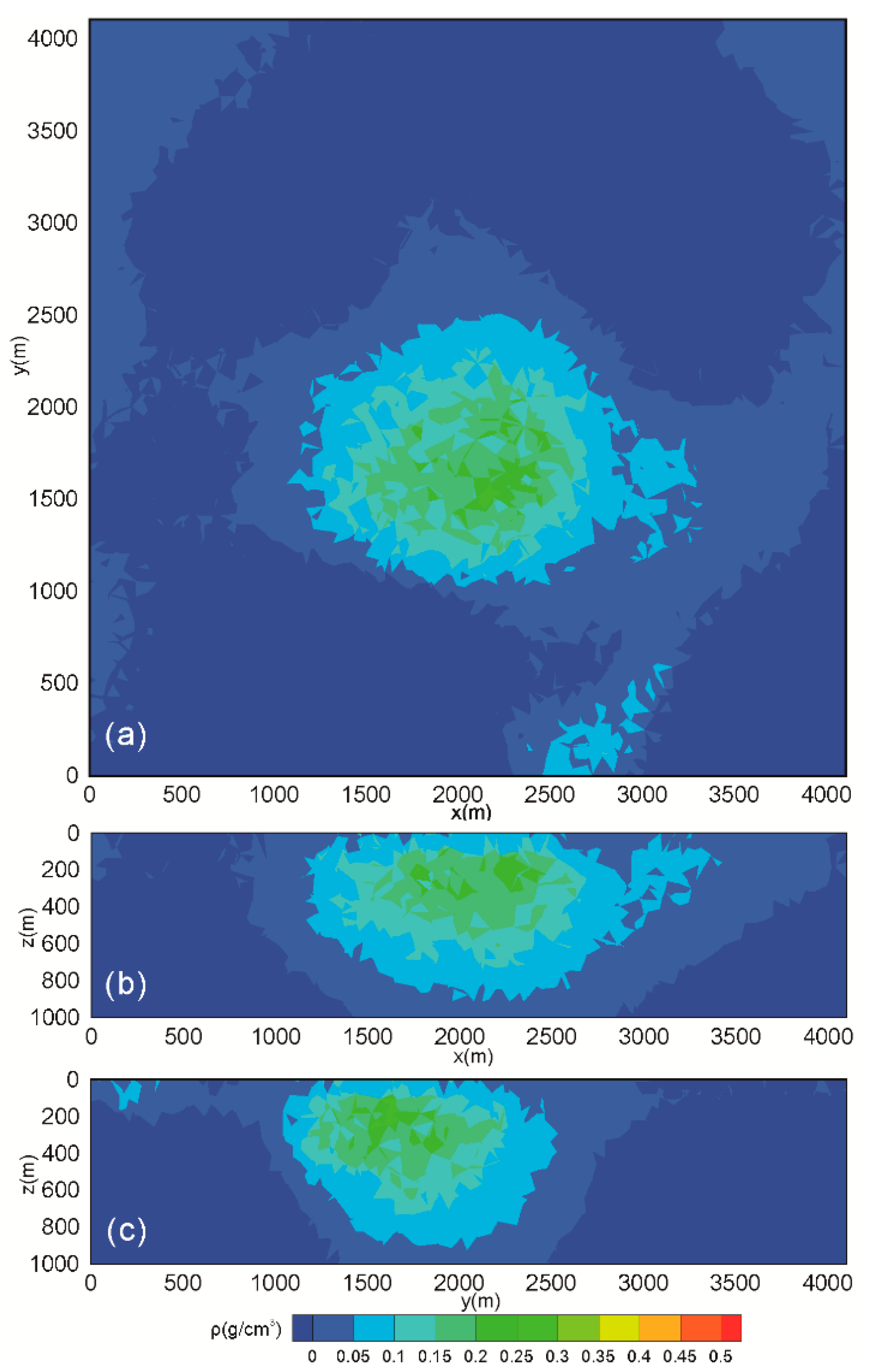
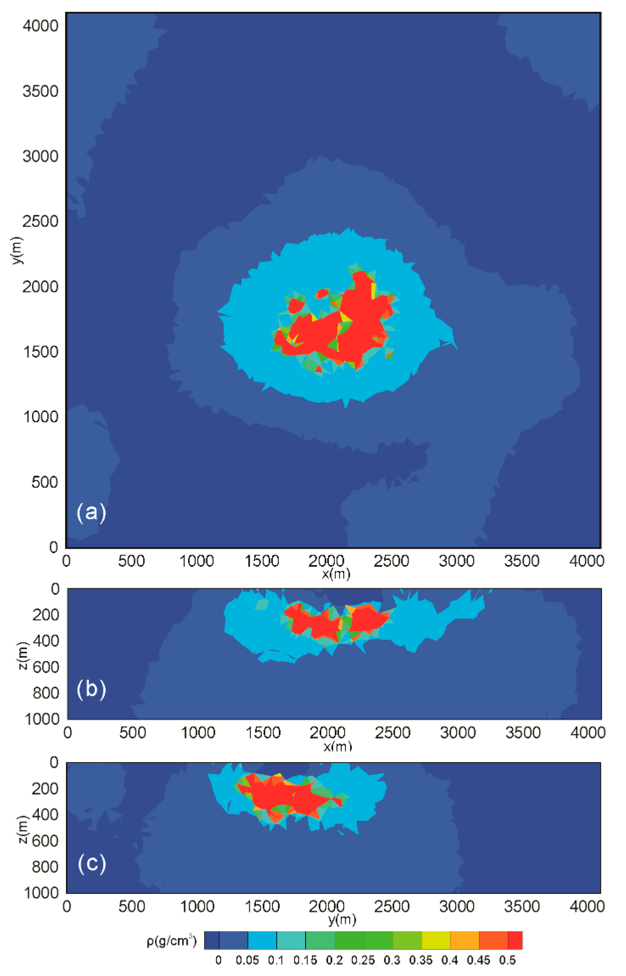
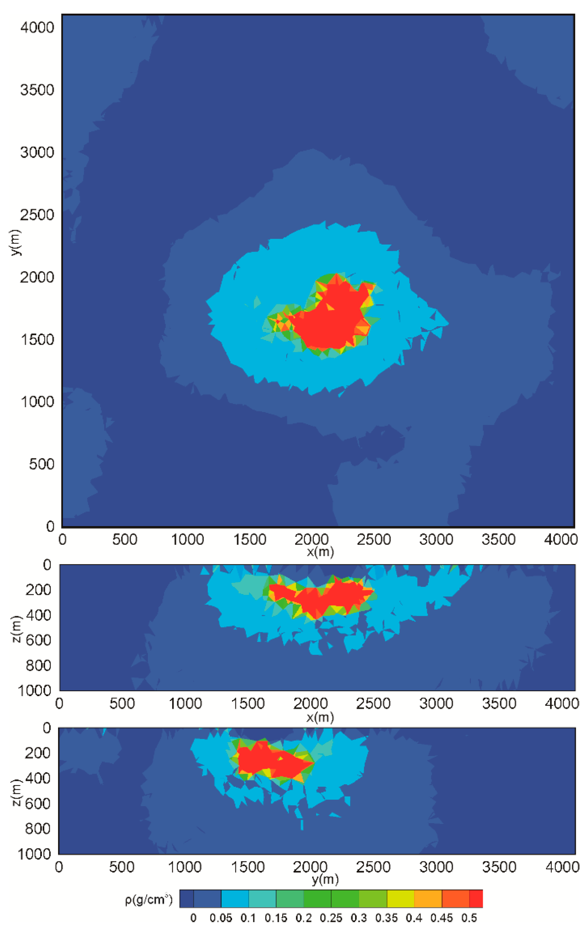
| Result | Inversion Method | Strategy | Trade-Off Parameter |
|---|---|---|---|
| Figure 4a | NaN | Conventional strategy | 0 |
| Figure 4b | NaN | Gradient-based strategy | 0 |
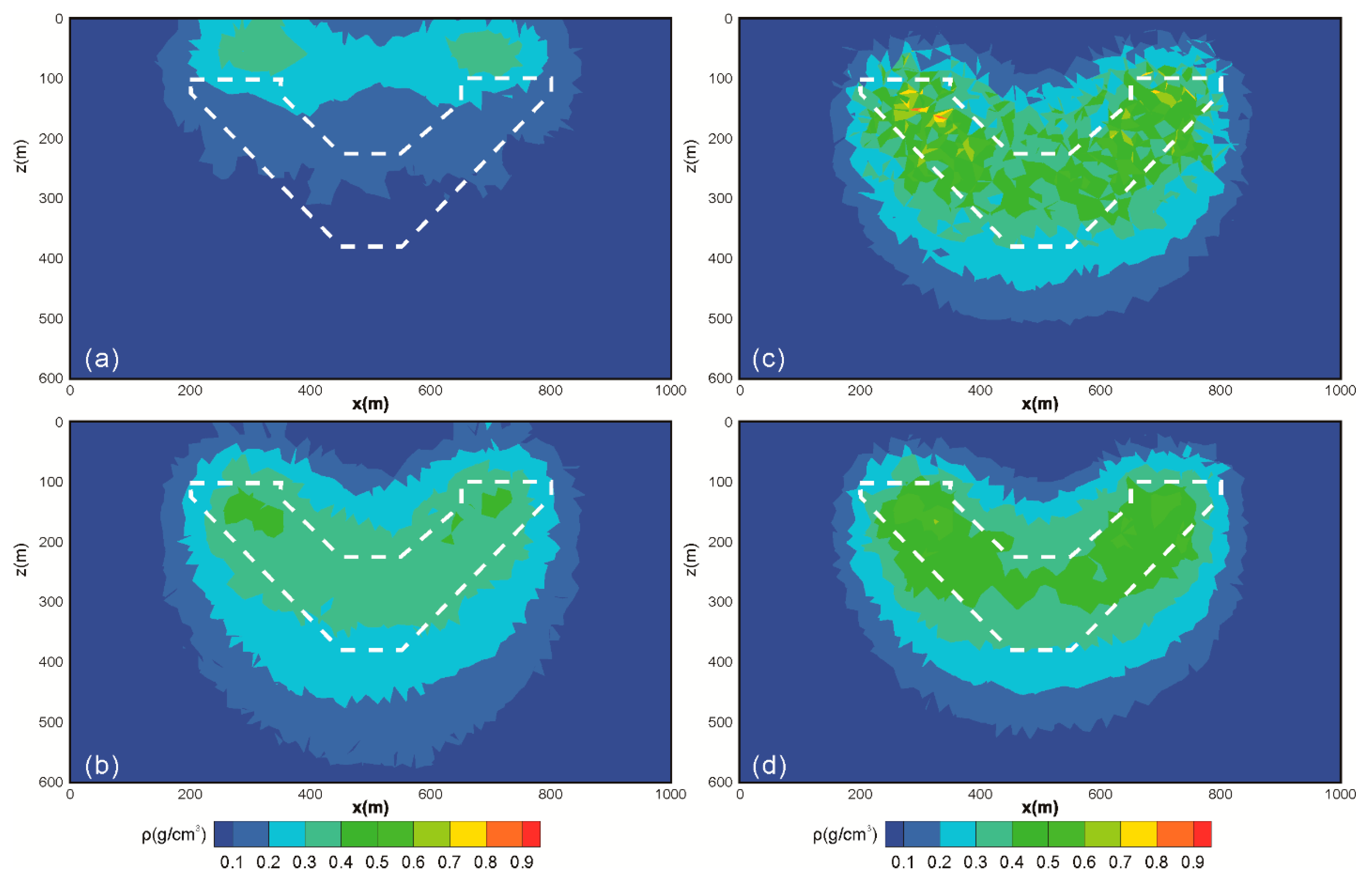
| Figure 5a | Smooth inversion | Conventional strategy | 1 × 10⁻² |
| Figure 5b | Smooth inversion | Conventional strategy | 5 × 10⁻² |
| Figure 5c | Smooth inversion | Gradient-based strategy | 1 × 101 |
| Figure 5d | Smooth inversion | Gradient-based strategy | 5 × 101 |
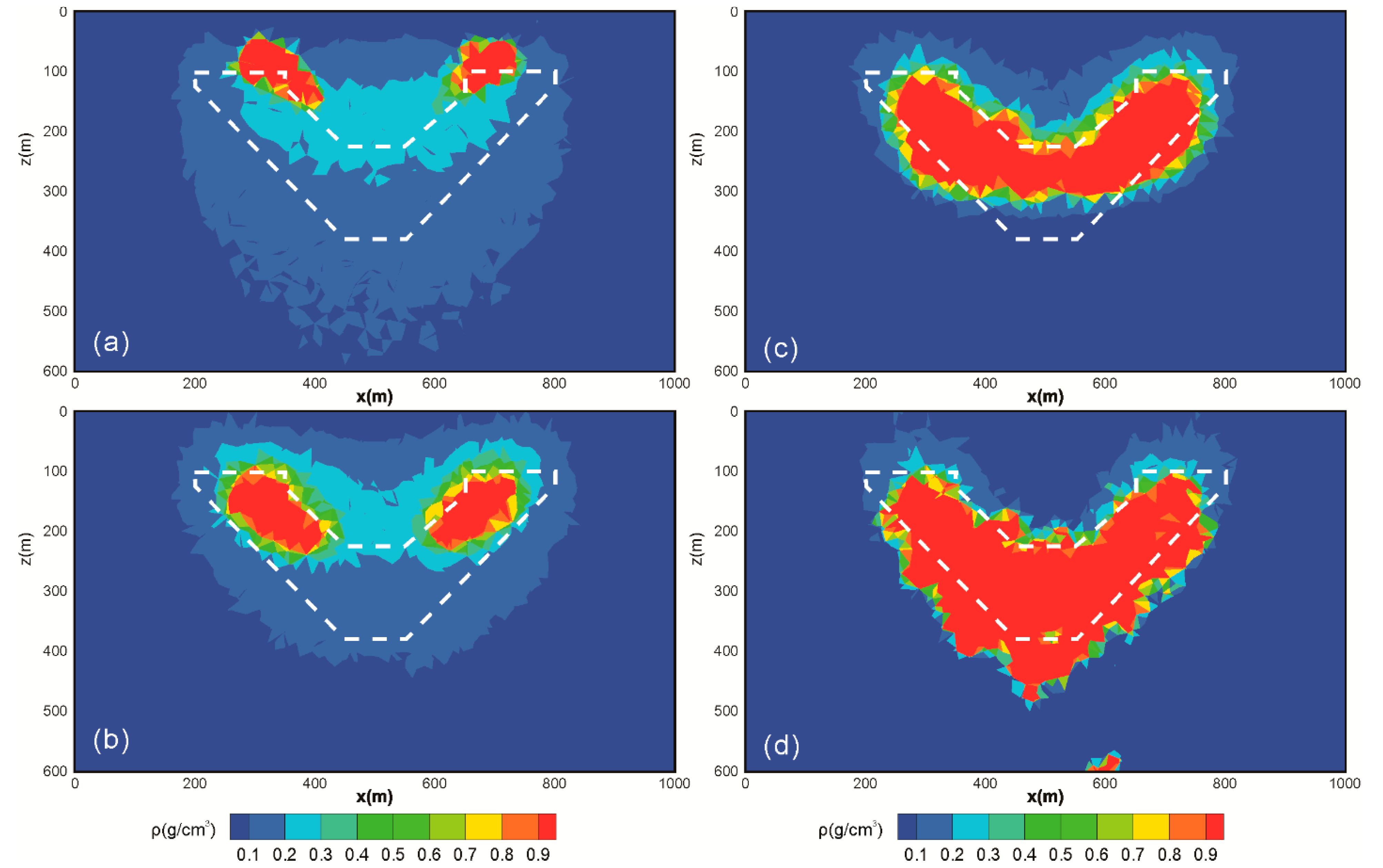
| Figure 6a | New FCM inversion | Conventional strategy | 1 × 10⁻³ |
| Figure 6b | New FCM inversion | Conventional strategy | 3 × 10⁻³ |
| Figure 6c | New FCM inversion | Gradient-based strategy | 3 × 100 |
| Figure 6d | New FCM inversion | Gradient-based strategy | 5 × 100 |
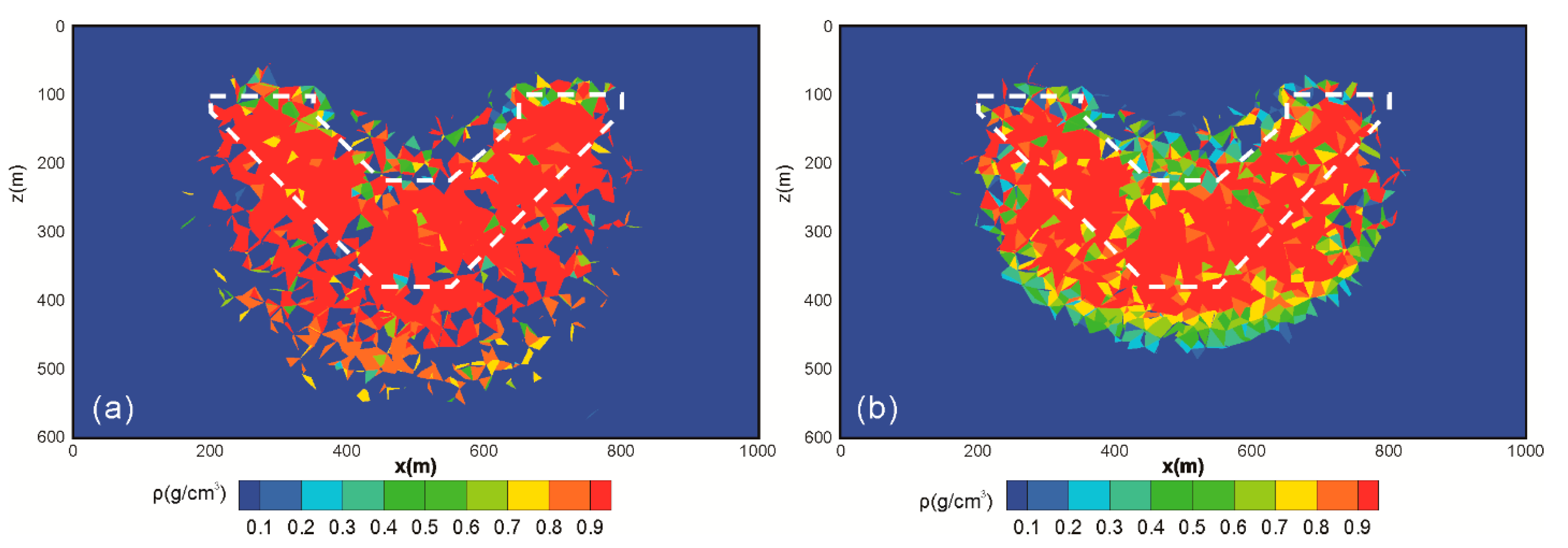
| Figure 7a | Focusing inversion | Gradient-based strategy | method of Lelièvre et al. [17] |
| Figure 7b | Conventional FCM inversion | Gradient-based strategy | method of Lelièvre et al. [17] |
Publisher’s Note: MDPI stays neutral with regard to jurisdictional claims in published maps and institutional affiliations. |
© 2021 by the authors. Licensee MDPI, Basel, Switzerland. This article is an open access article distributed under the terms and conditions of the Creative Commons Attribution (CC BY) license (http://creativecommons.org/licenses/by/4.0/).
Share and Cite
Sun, S.; Yin, C.; Gao, X. 3D Gravity Inversion on Unstructured Grids. Appl. Sci. 2021, 11, 722. https://doi.org/10.3390/app11020722
Sun S, Yin C, Gao X. 3D Gravity Inversion on Unstructured Grids. Applied Sciences. 2021; 11(2):722. https://doi.org/10.3390/app11020722
Chicago/Turabian StyleSun, Siyuan, Changchun Yin, and Xiuhe Gao. 2021. "3D Gravity Inversion on Unstructured Grids" Applied Sciences 11, no. 2: 722. https://doi.org/10.3390/app11020722
APA StyleSun, S., Yin, C., & Gao, X. (2021). 3D Gravity Inversion on Unstructured Grids. Applied Sciences, 11(2), 722. https://doi.org/10.3390/app11020722