Research on Segmentation and Classification of Heart Sound Signals Based on Deep Learning

Abstract

The heart sound signal is one of the signals that reflect the health of the heart. Research on the heart sound signal contributes to the early diagnosis and prevention of cardiovascular diseases. As a commonly used deep learning network, convolutional neural network (CNN) has been widely used in images. In this paper, the method of analyzing heart sound through using CNN has been studied. Firstly, the original data set was preprocessed, and then the heart sounds were segmented on U-net, based on the deep CNN. Finally, the classification of heart sounds was completed through CNN. The data from 2016 PhysioNet/CinC Challenge was utilized for algorithm validation, and the following results were obtained. When the heart sound segmented, the overall accuracy rate was 0.991, the accuracy of the first heart sound was 0.991, the accuracy of the systolic period was 0.996, the accuracy of the second heart sound was 0.996, and the accuracy of the diastolic period was 0.997, and the average accuracy rate was 0.995; While in classification, the accuracy was 0.964, the sensitivity was 0.781, and the specificity was 0.873. These results show that deep learning based on CNN shows good performance in the segmentation and classification of the heart sound signal.

1. Introduction

The heart sound results from myocardial movement and the valve opening and closing; it is greatly affected by the hemodynamics and electrical activity of the heart muscle [1]. In the early stage of cardiovascular disease, heart sound auscultation, as a means of preliminary screening for cardiovascular diseases, can help differentiate abnormal signals from normal heart sound signals, and, therefore, provide effective information for the auxiliary diagnosis of cardiovascular diseases. Any dysfunction and anatomical defect in the heart can be reflected by the time, frequency spectrum, and morphological characteristics of the heart sound [2]. Though the electrocardiogram (ECG) signal contains a lot of physiological information on the cardiovascular system, it cannot reveal a lesion in the early stage of cardiovascular disease, for a lesion is not clear enough. Yet, this can be achieved by heart sounds during the early stage of the lesion. Therefore, heart sound signals contain very important physiological information, and the study of heart sound signals possesses very important clinical value for the early diagnosis of cardiovascular diseases. The segmentation and classification of heart sound signals are currently the most commonly used methods for studying the heart sound signal.

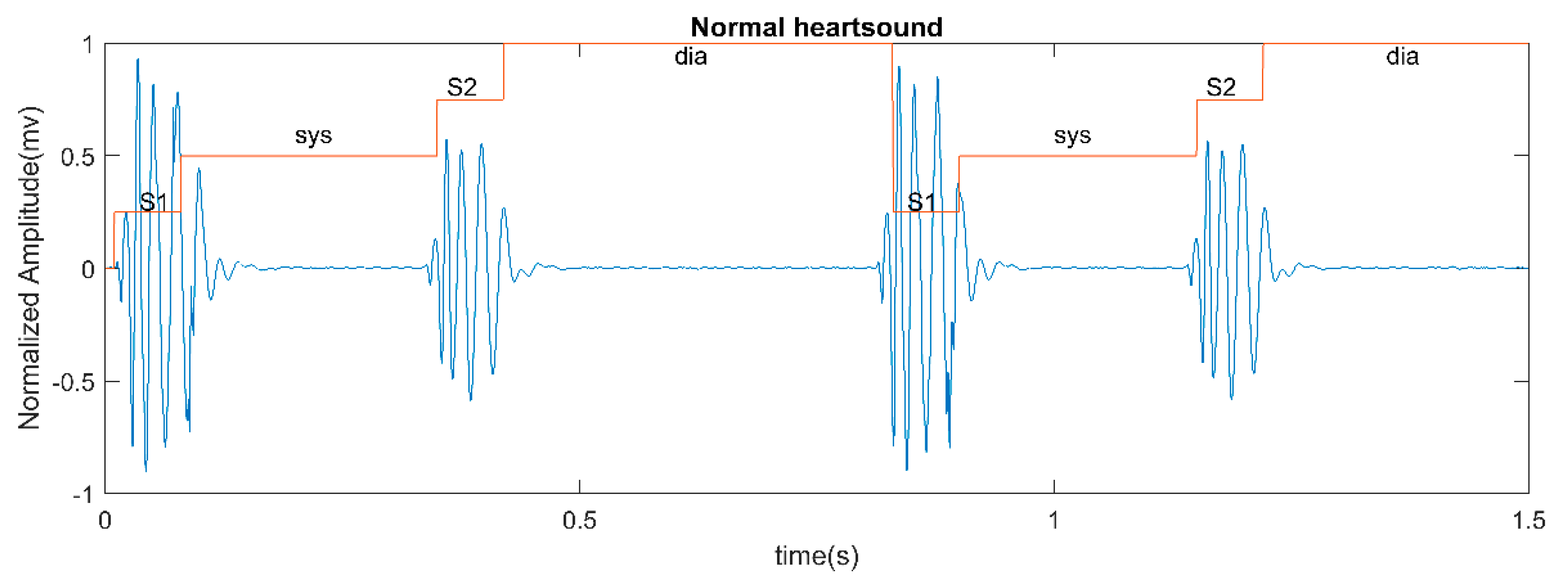
Heart sound segmentation, as a common method of heart sound signal processing, aims to divide the heart sound cycle into four corresponding states, and it is also an important processing step for heart sound classification [3]. A heart sound cycle of a normal adult mainly includes the first heart sound (S1), systolic period (sys), the second heart sound (S2), and diastolic period (dia), as shown in Figure 1. S1 occurs when the mitral and tricuspid valves close, which marks the beginning of ventricular contraction. S2 occurs when the aortic valve and pulmonary valve close, marking the beginning of ventricular diastole. The normal contraction and relaxation of the heart are the basis of human blood circulation. When there are abnormalities in the heart, they will be shown in the heart sound signal, and various diseases have different signals. For example, for several common heart valve diseases, the manifestations of heart sounds is that there are often murmurs appearing in mitral regurgitation during systole, mitral valve stenosis during diastole, pulmonary valve stenosis during systole, ventricular septal defect during diastole, aortic valve stenosis during systole, and in aortic valve insufficiency during diastole. Based on the abnormal part of the heart sound, experienced clinicians can make a preliminary diagnosis of the disease, with some necessary examinations according to the needs of the patient for further diagnosis. The determination of the abnormal part of the heart sound can only be achieved when the state of the heart sound is determined, which can be done by heart sound segmentation. The common methods for heart sound segmentation mainly includes ECG signal-based segmentation methods [4,5,6], envelope-based segmentation methods [7,8,9,10,11], feature-based segmentation methods [12,13,14,15], machine learning-based segmentation methods [16,17,18,19,20], and Hidden Markov Model (HMM)-based segmentation methods [16,21,22,23,24]. In earlier times, there has been only some achievements made in segmentation methods based on ECG signals and envelopes. Later, Schmidt et al. first used the Hidden semi-Markov Model (HSMM) to precisely simulate the expected duration of HMM center sounds [23]. Based on the research of Schmidt et al., Springer et al. extended this method through using logistic regression’s emission probability estimation, improving the Viterbi algorithm to decode the most probable heart sound state sequence, and obtained HSMM based on logistic regression (LR-based HSMM) [24]. Until 2016, this method has been regarded as a very good method for heart sound signal segmentation, which was recommended as the heart sound signal segmentation algorithm by The 2016 PhysioNet/CinC Challenge. Many people who participated in the competition used this method for segmentation before classifying heart sounds, and got a good ranking. [25,26,27]. However, for this method, the prediction time of each state needs to be added, and the logistic regression based on the Gaussian distribution of emission probability estimation and the extended Viterbi algorithm are used to predict the next states [24], and there will be errors in this method in the case of long period and irregular sinus rhythm [20]. However, the method based on convolutional neural network (CNN) does not require preliminary detection of the Phonocardiogram (pcg) segment. The structure of CNN is directly used to obtain the sound characteristics able to minimize segmentation errors from the heart sound signal itself or the features extracted from it, when completing the segmentation of the heart sound [19].

Heart sound classification is to determine whether a heart sound is normal or not. The classification method of heart sounds includes heart sound classification without segmentation and heart sound classification including segmentation. Heart sound classification without segmentation means that the features of the entire heart sound are extracted after the preprocessing of the heart sounds, and the classifier is trained and classified using these features. In recent years, Hamidi, Arora, and Yaseen et al. have conducted some related research [28,29,30]. Heart sound classification including segmentation is to extract the features of S1, sys, S2, and dia, based on the segmentation of the heart sound, and a new feature set is formed through the combination of these features of each part and other features of the entire heart sound. The classifier is trained and classified based on the new feature set. In this aspect, Pedro Narváez, Kucharski, and Li Fan et al. have done related work [31,32,33]. Compared with the heart sound classification without segmentation, the heart sound classification including the segmentation can obtain the state mark of the heart sound, which enables the clinicians to locate the abnormality part of the heart sound, such as diastolic or systolic murmur, and contributes to further determining the position of the heart valve that results in the disease. “classification of heart sound recordings-the physionet computing in cardiology challenge 2016” was a competition for heart sound classification [34], aiming to encourage the development of algorithms to classify heart sound recordings and to identify whether the subject of the recording should be referred on for an expert diagnosis. The PhysioNet provides a basic method for heart sound segmentation and a large number of heart sound signals, which have been widely applied in the 2016 competition and other researches afterwards. Among the participants in the competition, Potes et al. used the segmentation algorithm to classify heart sounds and obtained the first place [25]. However, in subsequent research on heart sound signals, Renna et al. pointed out that the complex sound classifier can only improve the classification to a limited extent, and the improved segmentation algorithm can be the best way of obtaining a more significant improvement in heart sound classification. They applied CNN to heart sound signal segmentation and got good experimental results, but they did not further discuss whether the segmentation network leads to a good performance of classification [19]. In 2020, Khan et al. also studied heart sound signals. They compared the classification results of segmented and unsegmented heart sound signals and concluded that using segmented heart sound signals can contributes to better classification. However, in the experiment, they used the improved empirical wavelet transformation and standardized Shannon average energy to preprocess and automatically segment the signals to identify the systolic and diastolic interval of the signal, instead of the segmentation of the four states [35].

Therefore, this paper studies the method of heart sound segmentation using deep CNN, and further combines the segmentation network with heart sound classification. Firstly, the heart sound was preprocessed, then the signal was segmented in the multi-channel deep CNN, and finally classified in the CNN classifier and the Adaboost classifier. Heart sound segmentation, as a necessary stage of heart sound signal analysis, does not require the knowing of prediction time of each state in advance, and directly uses the deep CNN to learn the sound features that minimize segmentation errors, which is the focus of this paper. Considering the increasing number of cardiovascular diseases and the existing shortage of medical resources, we will apply a relevant study to real life by a set of auxiliary diagnosis system including hardware and software, as shown in Figure 2. The hardware mainly includes electronic stethoscope (simple electronic stethoscope and professional electronic stethoscope), and the software includes record analysis software on the computer and mobile phones. The simple electronic stethoscope is available in every household just like a clinical thermometer. When the body is abnormal, the device is used to collect the signal and gets a preliminary diagnosis on the mobile terminal of the mobile phone. If the signal is abnormal, people who was uncomfortable go to the hospital for treatment. In hospital, the doctor collects the signal through the professional equipment, analyzes the signal on the computer (just like the ECG), and arranges the next examination.

2. Materials and Methods

2.1. Pre-Processing of Signal

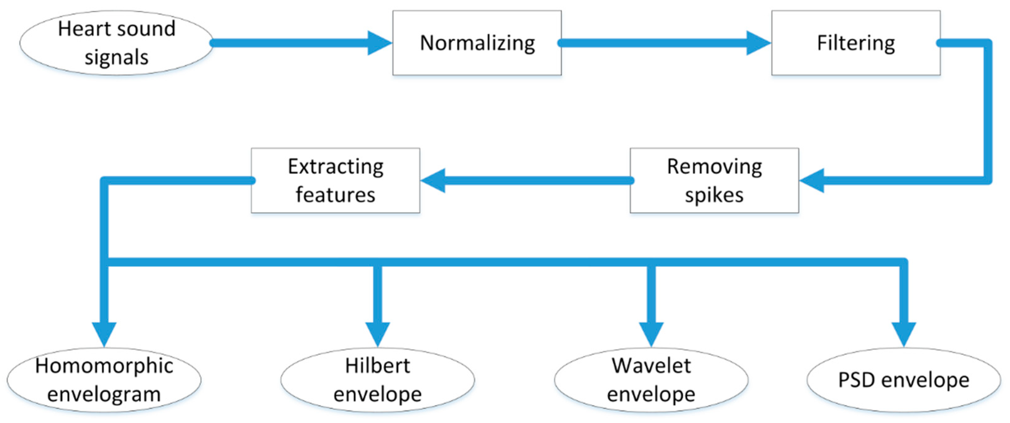
The heart sounds is preprocessed to produce the data meeting the requirements of model input, which is shown in Figure 3. First, normalize the data to eliminate the influence on amplitude changes the differences in acquisition technology and auscultation location exert. This paper used normalization technique to reduce the difference between different data to the largest extent, as expressed in Equation (1).

$$x(n)=\frac{x_r(n)-x_r(\min )}{x_r(\max )-x_r(\min )}$$

(1)

where x_r(n) represents the original heart sounds signal, and x(n) represents the normalized heart sounds signal. While x_r(min) and x_r(max) are the minimum and maximum values of the original signal, respectively.

Then, second-order high-pass and low-pass Butterworth filters with cut-off frequencies of 25 Hz and 400 Hz were used to filter the normalized heart sounds signal, and spike removal and feature extraction were used for the filtered signal. The four methods were used to extract features: (1) Hilbert envelope; (2) Homomorphic environment map; (3) Wavelet envelope; (4) Power spectral density envelope.

Finally, the obtained features were down-sampled to 50 Hz, and all down-sampled features were normalized in order to obtain zero mean and unit variance [9]. For each feature envelope obtained, the fixed length is extracted according to the overlapping step length of adjacent data, which can be expressed in Equation (2).

$$X_k(n)=\left[\begin{array}{c}{x}_k^{\prime }((n-1)\cdot \tau -\frac{n-1}{8}\cdot \tau -(n-2))\\ ⋮\\ x_k^{\prime }((n\cdot \tau -\frac{n-1}{8}\cdot \tau -(n-1)))\end{array}\right]$$

(2)

where $x_k^{\prime }$ is the feature of the original length of the data, X_k represents the feature of extracting fixed-length data, k = 1,2,3,4, n = 1,2, …, $\frac{8\cdot N-\tau -8}{7\cdot \tau -8}$, and N represents the total length of the data, and $\tau$ is the fixed length of the data input to the model.

2.2. Segmentation of Signal

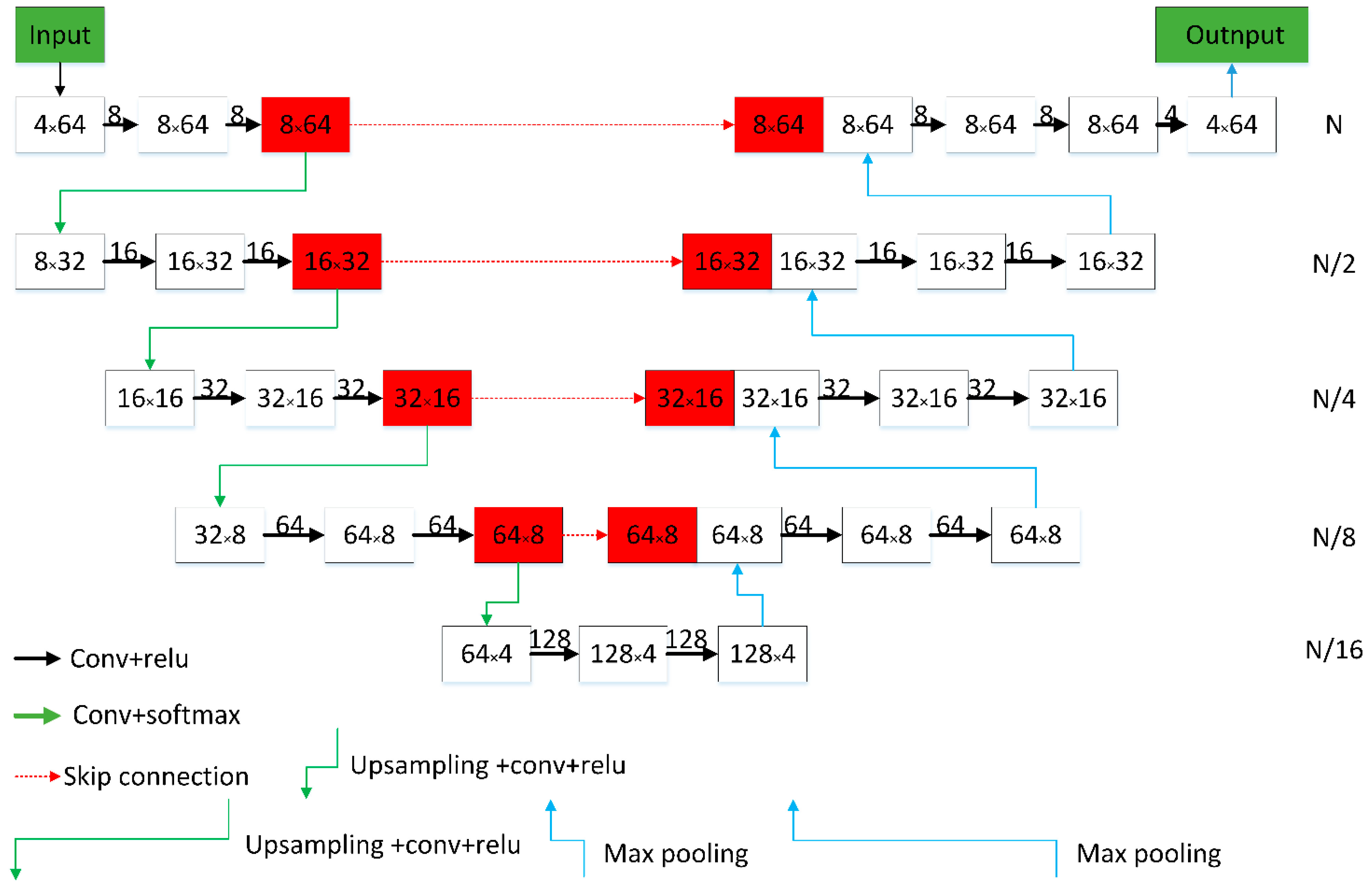
Heart sound segmentation, which segmented the heart sounds into 4 periods (including S1, systolic, S2, and diastolic) based on the features obtained through preprocessing, was the focus of this paper. This paper adopted U-net implementation based on the deep CNN, as is shown in Figure 4. Additionally, the network structure is shown in Figure 5.

The mathematical model of the convolution of each layer of the network in this architecture can be expressed in Equation (3):

$$Z_{i,j}^{\ell }={\displaystyle \sum _{i=1}^{N^{\ell }}{\displaystyle \sum _{j=1}^{k^{\ell }}{A}_{i,j}^{\ell }}}{W}_{i,j}^{\ell }$$

(3)

where A_i,j represents the element in the i-th row and j-th column of the matrix, the elements of matrix A correspond to the weights of different filters corresponding to different feature inputs of the $\ell$-th layer, and $N^{\ell }$ represents the dimension of the input feature space of the $\ell$-th layer, $k^{\ell }$ represents the output feature space dimension of the $\ell$-th layer, and $W_{i,j}^{\ell }$ and $Z_{i,j}^{\ell }$ represent the input and output of the $\ell$-th convolutional layer, respectively.

The network can be understood as down-sampling, up-sampling, splicing, and fusion. Specifically, down-sampling implemented different degrees of convolution operations and learnt features at different levels. As the depth of the network increases, the learned features were also converted from low-dimension to high-dimension; Up-sampling implemented the deconvolution. After learning the deep features, the data length were gradually restored to the size of the original inputs; The splicing fusion combined the different dimensional features learned by down-sampling with the recovered data from up-sampling to realize the fusion of features at different scales. Finally, the network output was followed by a softmax activation function, and the output was each state sequence corresponding to the heart sound.

It should be noted that the output of all convolutional layers of the network needed to be zero-filled to ensure that the data space dimension does not change after convolution, as shown in Figure 6.

2.3. Classification

The heart sound segmentation was realized by completing the heart sound labeling. There were many ways to classify heart sounds based on segmentation, and this study chose the adaboost classifier and CNN classifier to achieve the classification of heart sounds. Adaboost is an iterative algorithm. Its core idea is to train different classifiers (weak classifiers) for the same training set, and then these weak classifiers are grouped to form a stronger final classifier (strong classifier). The CNN classifier was implemented by constructing a network structure of a series of multi-layer convolutional layers and multi-layer perceptrons (MLP). In the multi-layer convolutional layer, sufficient features were obtained by controlling the number of convolution kernels, and the obtained features were inputted into the MLP network to classify heart sounds. The process is shown in Figure 7.

2.4. Network Model

To conduct a comprehensive study of the characteristics of the heart sound signals, this paper established the segmentation and classification model structure based on CNN. The input layer was the four features extracted after pre-processing. The four features with a fixed length of 512 were selected as the input of the multi-channel CNN, which were divided into corresponding states by the segmentation network, and then connected to the CNN classifier to complete the classification. The network structure consisted of three parts, including pre-processing, a U-net segmentation network based on the deep CNN, a CNN classifier. The overall flow chart is shown in Figure 8.

3. Experiment

3.1. Data Sources

The data used in this paper were from the 2016 PhysioNet/CinC Challenge database [29], which provided segmentation and classification annotations. It is currently the world’s largest public heart sound data set. Among them, a total of 792 pieces of data with segmentation annotations were stored at a sampling frequency of 1 kHz, and a total of 301 pieces of heart sounds with classification annotations were stored at a sampling frequency of 2 kHz.

3.2. Data Pre-Processing

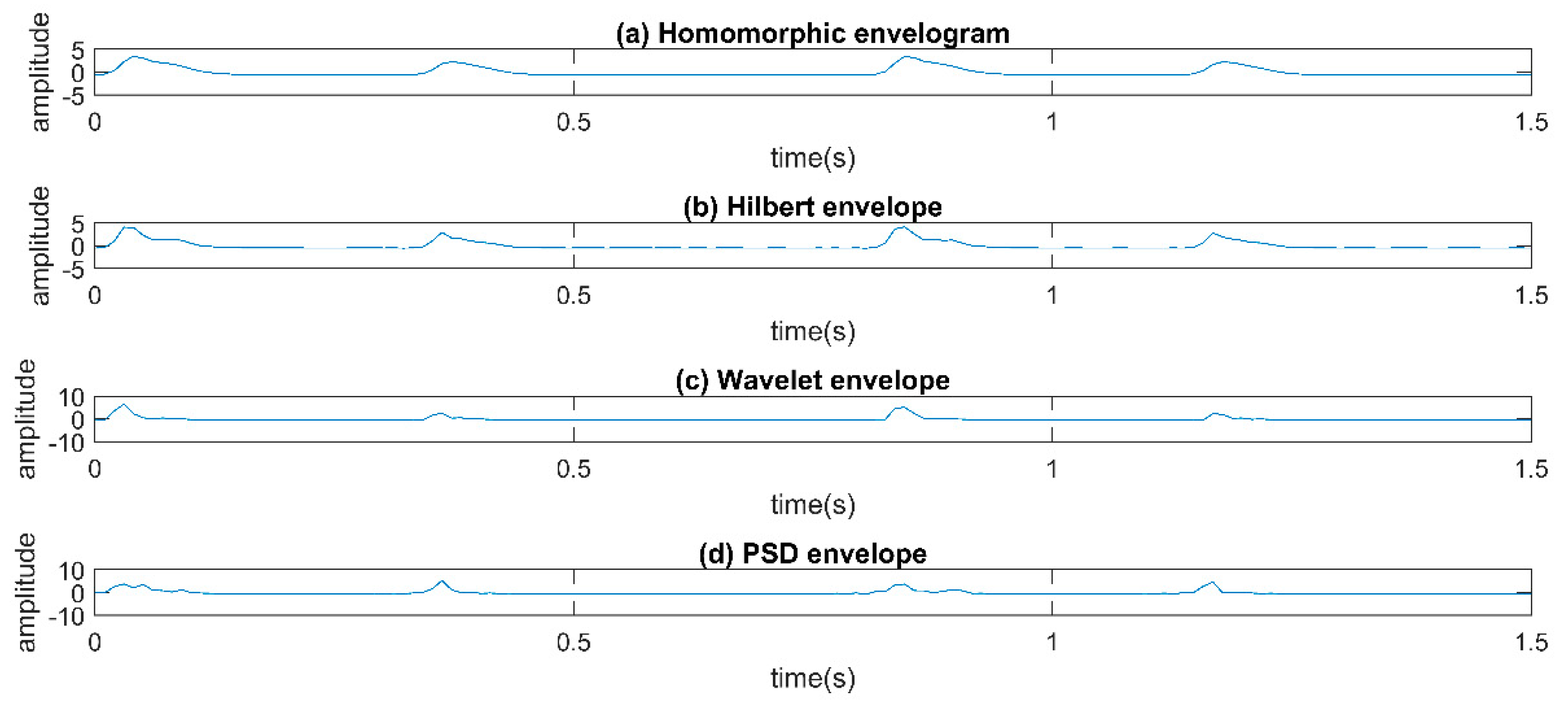
Referring to the process of signal pre-processing, the fixed length values in this paper were 64, 128, 256, and 512. The overlapping steps of two adjacent data was 1/8 of the fixed length.

Table 1. The number of data obtained with different fixed lengths.

Length	64	128	256	512
Number	8431	3936	1725	711

corresponds to the number of data with different fixed lengths, and the Figure 9 shows the envelope extracted from a heart sound. In order to improve the effectiveness utilization of data and increase the robustness of the algorithm model, this paper used a 10-fold cross-validation method.

3.3. Evaluation Index

To analyze the results of the model, this paper used the following six indicators: overall accuracy (PA), accuracy of each state (CPA), and average accuracy of each state (MPA), accuracy (Acc), sensitivity (Se), and specificity (Sp). Among them, PA, CPA and MPA were used for the evaluation of segmentation performance, while Acc, Se, and Sp were used to evaluate the classification performance. The relevant indicators are calculated as follows.

$$PA=\frac{T_P+T_N}{T_P+T_N+F_P+F_N}$$

(4)

$$CPA=\frac{T_P}{T_P+F_P}$$

(5)

$$MPA=\frac{1}{4}{\displaystyle \sum _{i=1}^{4}CP{A}_i=\frac{1}{4}{\displaystyle \sum _{i=1}^4\frac{T_P}{T_P+F_P}}}$$

(6)

$$Acc=\frac{T_P+T_N}{T_P+T_N+F_P+F_N}$$

(7)

$$Se=\frac{T_P}{T_P+F_N}$$

(8)

$$Sp=\frac{T_N}{T_N+F_P}$$

(9)

where T_P represents the number of normal and classified as normal, F_P represents the number of abnormal but classified as normal, T_N represents the number of abnormal and classified as abnormal, and F_N represents the number of normal but classified as abnormal.

4. Results

4.1. Development Environment

The Experimental configuration environment was as follows: Intel Core [email protected] CPU, 8G RAM, and a GTX 550 graphics card. The Python 3.7 was selected as the development platform, and used the pytorch as the back-end.

4.2. Impact of Fixed Length on Performance Indicators

During the experiment, this study set up input signals of four lengths to train and test the model. The set signal lengths were 64, 128, 256, 512 (corresponding to 1.28 s, 2.56 s, 5.12 s, 10.24 s, respectively).

Table 2. Experimental results under different lengths.

Length	PA	CPA	MPA
64	0.895	[0.848 0.873 0.842 0.934]	0.874
128	0.918	[0.864 0.923 0.889 0.942]	0.904
256	0.991	[0.976 0.995 0.995 0.992]	0.990
512	0.994	[0.986 0.993 0.994 0.996]	0.992

shows the results. It was found out that when the length was set to 512, the best results were obtained: the accuracy of segmentation was 0.994, and the accuracy of the four states of S1, sys, S2, and dia were 0.986, 0.993, 0.994, and 0.996, respectively. The average accuracy rate was 0.992.

From these results, it can be seen that the performance of all aspects was significantly improved when the length was 512. In addition, in Table 1, it can be seen that when the length was set to 512, there were a total of 711 pieces of data, and the amount of data was significantly less than that of other lengths. However, Ronneberger et al. pointed out that the U-net network also showed good performance in small data sets [36]. Therefore, the input data length of the model was set to 512.

4.3. Impact of Optimizer on Performance Indicators

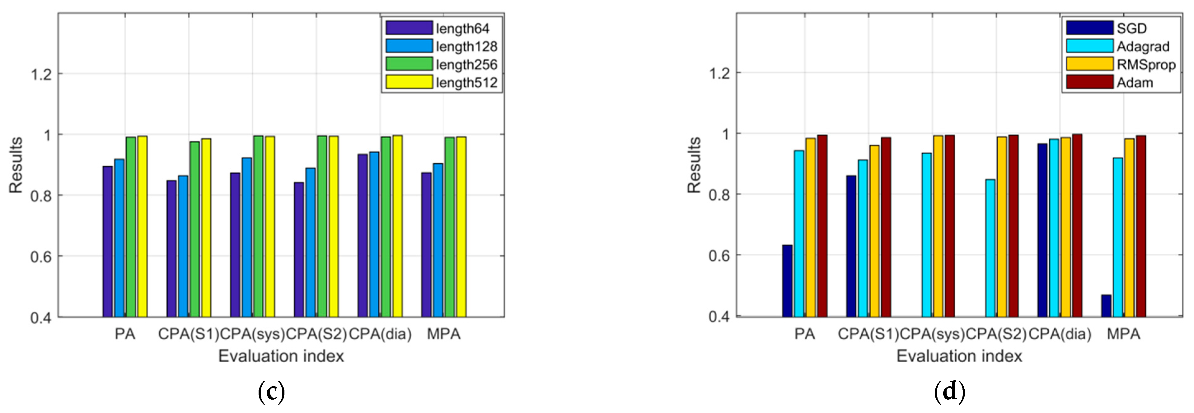
Through choosing a suitable optimizer and optimal learning rate, the training speed and classification accuracy of the model can be improved [37]. This article selected several commonly used optimizers—Adam, RMSprop (Root Mean Square Prop), Adagrad, and SGD (Stochastic Gradient Descent)—to train the model.

Table 3. The experimental results under different optimizer.

Optimizer	PA	CPA	MPA
SGD	0.632	[0.865 0.036 0.007 0.965]	0.468
Adagrad	0.943	[0.912 0.935 0.848 0.942]	0.980
RMSprop	0.983	[0.960 0.992 0.988 0.986]	0.982
Aadm	0.994	[0.986 0.993 0.994 0.996]	0.992

shows the experimental results under different optimizers. From these results, we can see that the segmentation effect was the best when the Adam optimizer was used, with the learning rate set to 0.0001.

4.4. Impact of U-net Depth on Performance Indicators

The U-net network was a network built on the basis of CNN. The increase in the number of network layers means an increase in the number of CNN. The deepened network can obtain higher-dimensional features. This paper set the depth of the U-net network to 5, 6, 7, and 8.

Table 4. Experimental results under different U-net depths.

Depth	PA	CPA	MPA
5	0.994	[0.986 0.993 0.994 0.996]	0.992
6	0.994	[0.985 0.996 0.996 0.997]	0.993
7	0.995	[0.989 0.993 0.996 0.998]	0.994
8	0.995	[0.987 0.995 0.996 0.996]	0.994

shows the experimental results under different U-net depths. As these results show, a good segmentation effect can be obtained in all depth parameters we set. However, considering the computer memory and training time, the depth was set to 5.

4.5. Impact of Convolution Kernel Sizes on Performance Indicators

Considering that the size of the convolution kernel has a deep influence on the classification performance and operation speed [37], four different convolution kernel were set after determining the basic structure of the network and the length of the input signal, which was shown in

Table 5. The experimental results under different convolution kernel sizes.

Convolution Kernel	PA	CPA	MPA
5 × 4	0.994	[0.986 0.993 0.994 0.996]	0.992
9 × 4	0.996	[0.991 0.996 0.996 0.997]	0.995
15 × 4	0.995	[0.987 0.997 0.996 0.996]	0.994
31 × 4	0.996	[0.991 0.995 0.994 0.998]	0.995

.

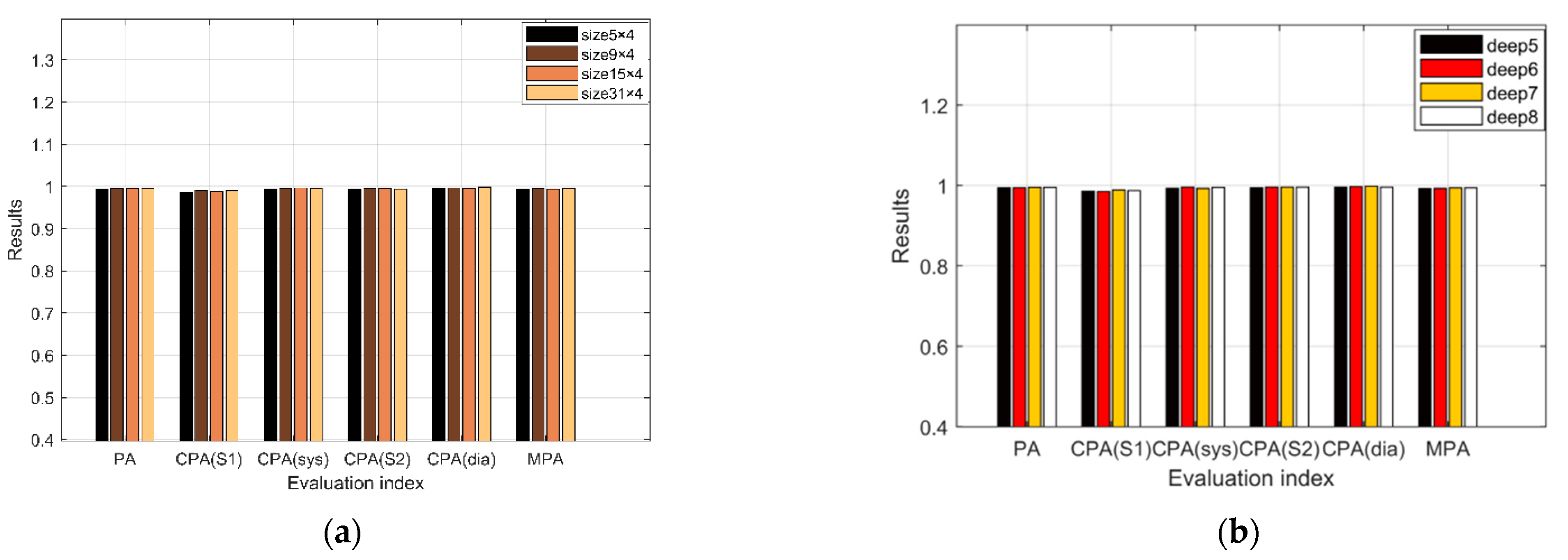
It was found out that the change of the convolution kernel has a certain influence on the result. When the convolution kernel is set to 9 × 4 and 31 × 4, the best segmentation effect was obtained. However, considering the influence of the increase in the size of the convolution kernel on the calculation speed, the model’s convolution kernel was set to 9 × 4 without wasting computing resources.

4.6. Determination of Segmentation Model Parameters

From the above experimental results, it can be seen that among all the parameters considered, the size and depth of the convolution kernel of the network have little influence on the segmentation effect, but the length of the input data and the selected optimizer possess a greater influence on the result, as shown in Figure 10.

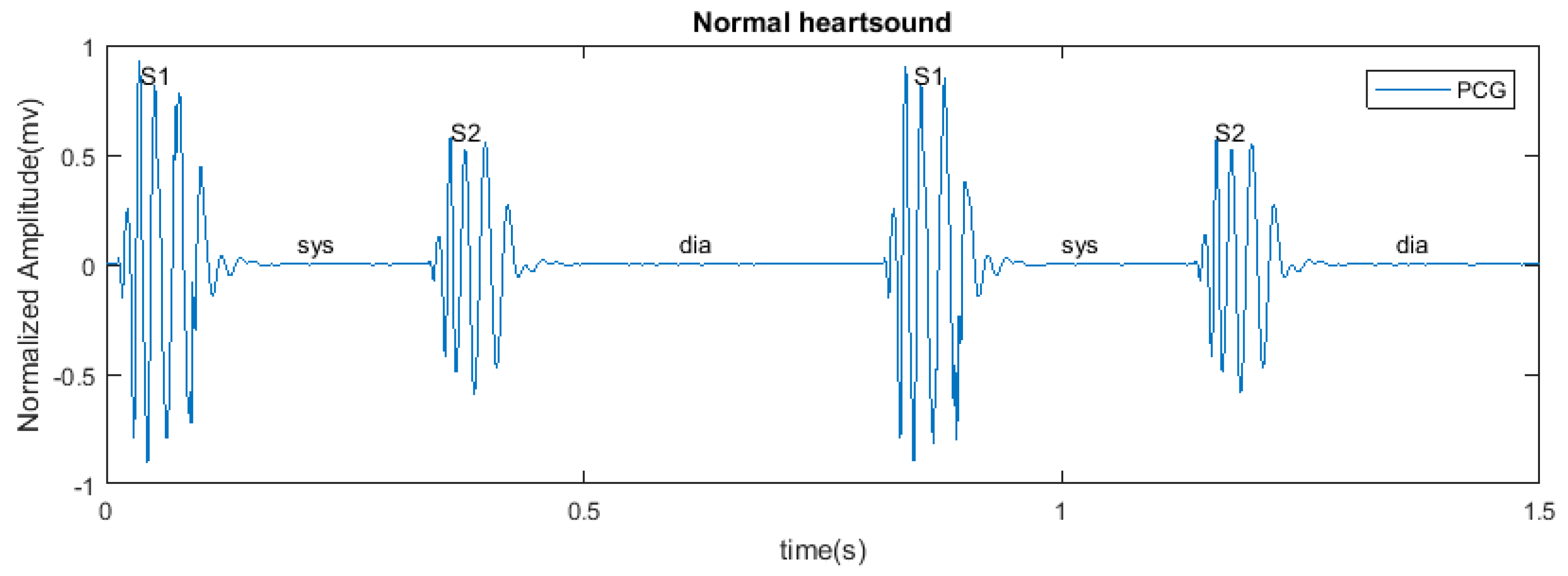
Finally, the segmentation model parameters were determined, as shown in

Table 6. Parameters setting of the segmentation model.

Deep	Type	Type	Filter Number	Kernel Size	Output Shape
1	Input	-	(8, 8)	9 × 4	8 × 512
2	Down1	(Conv + Zero padding) × 2 + max pooling	(16, 16)	9 × 4	16 × 512
3	Down2		(32, 32)	9 × 4	32 × 512
4	Down3		(64, 64)	9 × 4	64 × 512
5	Down4		(128, 128)	9 × 4	128 × 512
4	Up1	Up-sampling + Skip connection + (Conv + Zero padding) × 2	(64, 64)	9 × 4	64 × 512
3	Up2		(32, 32)	9 × 4	32 × 512
2	Up3		(16, 16)	9 × 4	16 × 512
1	Up4	Up-sampling + Skip connection + (Conv + Zero padding) × 3	(8, 8, 4)	9 × 4	8 × 512
1	Output	Soft max	4	9 × 4	4 × 512

. The length was 512, the optimizer Adam was chosen, the network depth was 5, and the convolution kernel was 9 × 4. Figure 11 shows the segmentation result of a normal heart sound. In the process of down-sampling, the number of filters in the convolutional layer increased from 8 to 128 successively, and in the process of up-sampling, the number of filters was sequentially reduced from 128 to 4; the size of the convolution kernel of each layer was 9 × 4, the stride of the convolution layer was 1, the pooling layer was set to 2, and the learning rate was 0.0001.

4.7. Application of Segmentation Model in Classification

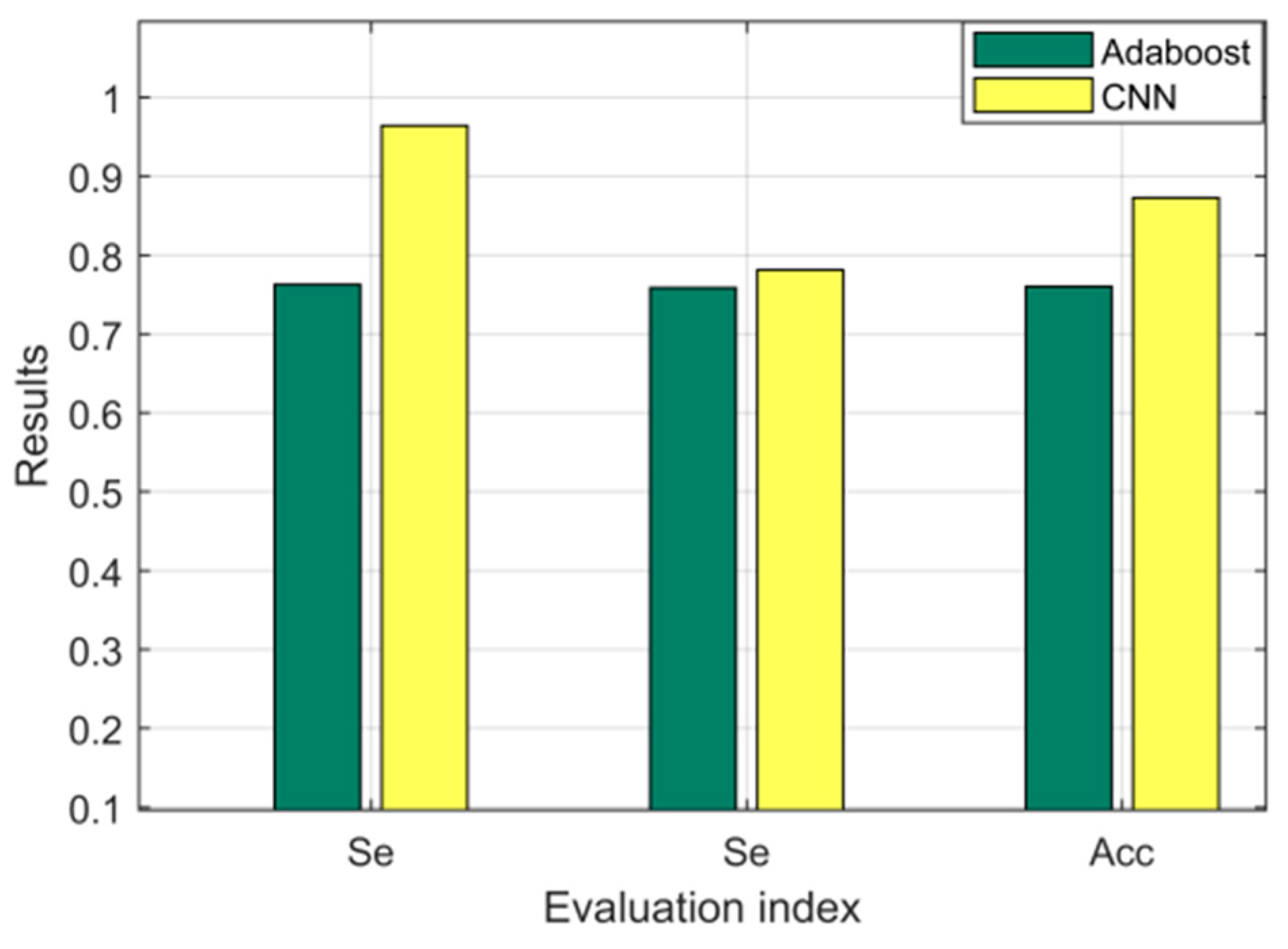
In this paper, the adaboost classifier and CNN classifier were selected on the basis of segmentation to classify heart sounds, and the classification results are shown in the following

Table 7. Classification results under different classifiers.

Classifier	Se	Sp	Acc
Adaboost	0.763	0.759	0.761
CNN	0.964	0.781	0.873

. It can be clearly seen from Figure 12. that the results of the CNN classifier are significantly better than the Adaboost classifier in sensitivity, specificity, and accuracy.

5. Discussion

In this paper, the CNN was used to segment the heart sound signal, and it was further applied to classification. In the study of heart sound signal segmentation, referring to the process of image segmentation, the U-net network composed of the deep CNN was used for the segmentation of heart sound. Furthermore, the CNN classifier was used to classify the segmented heart sounds into normal or abnormal. In terms of segmentation, we discussed the impact of data length, network depth, convolution kernel size, and optimizer on the segmentation results. It can be seen from the fixed length parameters that the increase in the data length can improve the segmentation accuracy. As Table 2 shows, the amount of data decreases while the fixed length increases. Ronneberger et al. pointed out that the U-net network can also show good performance on small data sets [36], with a smaller amount of data reducing the credibility of the optimized model. When the data length was set to 512, the best segmentation results were obtained. The influence of the amount of fixed-length data on the result needs to be further explored through more data. The increase in network depth can effectively improve the performance of the network. This conclusion is consistent with the research results obtained by Krizhevsky and Simonyan et al. [38,39]. However, during the experiment, it was found out that the increase in network depth will increase the complexity of the model. It means that the number of related parameters in the model has increased exponentially. Too many parameters will consume a lot of computer memory capacity and training time. On the basis of a good segmentation effect, it is not worthwhile to spend a lot of computer memory and training time on the improvement of the segmentation accuracy, which was why the network depth was set to 5. The selection of the optimizer has a greater impact on the segmentation results. When the SGD optimizer was selected, the segmentation results were poor. When the Adam optimizer was selected, the segmentation effect was improved to a certain extent, and it performed best in the selected optimizer. However, in the study conducted by Keskar et al., it can be found out that selecting the most basic SGD optimizer [40], and gradually increasing optimization parameters (such as first-order momentum, second-order momentum) to optimize the model according to the research object can improve the model. For heart sound signals, this method can be considered to further explore the optimizer of heart sound signals to further improve the performance of the model.

6. Conclusions

This paper proposed a method of using CNN to study heart sound signals, which mainly involved segmentation and classification. In the study of segmentation, this paper applied U-net network composed of deep CNN to the segmentation step, and determined the relevant parameters of the model and trained the model that can segment heart sounds well through optimizing the relevant network structure and comparing the segmentation results under different optimizers and different input data lengths. In the study of classification, the segmentation model obtained was used to segment the heart sounds, and then used the Adaboost classifier and the CNN classifier to classify the heart sounds, and finally compared the classification results to select a better classifier. Without knowing the prediction time of each state, the segmentation model we trained obtained the overall accuracy rate of 0.996, the accuracy rates of S1, sys, S2, and dia were 0.991, 0.996, 0.996, 0.997, and the average accuracy rate was 0.995. Additionally, in the subsequent classification process, the CNN classifier got the accuracy of 0.964, the sensitivity of 0.781, and the specificity of 0.873. Therefore, a preliminary conclusion can be drawn that, as a basic network structure of deep learning, CNN can be applied to the research of heart sounds. We also believe that it will shine in the future combination of heart sounds and deep learning. In addition, considering that the changes in heart sounds at different periods are often accompanied by different types of cardiovascular diseases, the advent of the era of big data, the rapid development of artificial intelligence and the increasing incidence of heart diseases, we can carry out the analysis of different types of diseases in the future, the study of heart sound signals in different periods, and even the research on specific diseases. In the future, we will focus on the study of heart sound signals in different periods, and expand the classification of normal and abnormal heart sounds to the screening of specific diseases in specific periods. At the same time, we will further look for more opportunities of collaboration with clinicians to collect more heart sound data, and optimize the model structure.

References

1. Kumar, D.K.; Carvalho, P.; Antunes, M.; Paiva, R.P.; Henriques, J. Noise detection during heart sound recording using periodicity signatures. Physiol. Meas. 2011, 32, 599–618. [Google Scholar] [CrossRef] [PubMed]
2. Rangayyan, R.M.; Lehner, R.J. Phonocardiogram signal analysis: A review. Crit. Rev. Biomed. Eng. 1987, 15, 211–236. [Google Scholar] [PubMed]
3. Dissanayake, T.; Fernando, T. Understanding the importance of heart sound segmentation for heart anomaly datec-tion. arXiv 2020, arXiv:2005.10480v1. [Google Scholar]
4. Lehner, R.J.; Rangayyan, R.M. A Three-Channel Microcomputer System for Segmentation and Characterization of the Phonocardiogram. IEEE Trans. Biomed. Eng. 1987, BME-34, 485–489. [Google Scholar] [CrossRef] [PubMed]
5. Ahlström, C.; Länne, T.; Ask, P.; Johansson, A. A method for accurate localization of the first heart sound and possible applications. Physiol. Meas. 2008, 29, 417–428. [Google Scholar] [CrossRef] [PubMed]
6. Ahlström, C.; Hult, P.; Rask, P.; Karlsson, J.-E.; Nylander, E.; Dahlström, U.; Ask, P. Feature Extraction for Systolic Heart Murmur Classification. Ann. Biomed. Eng. 2006, 34, 1666–1677. [Google Scholar] [CrossRef] [Green Version]
7. Liang, H.; Lukkarinen, S.; Hartimo, I. Heart sound segmentation algorithm based on heart sound envelo-gram. IEEE 1997, 24, 105–108. [Google Scholar]
8. Huiying, L.; Sakari, L.; Iiro, H. A heart sound segmentation algorithm using wavelet decomposition and recon-struction. In Proceedings of the International Conference of the IEEE Engineering in Medicine & Biology Society, Chicago, IL, USA, 30 October–2 November 1997. [Google Scholar]
9. Maglogiannis, I.; Loukis, E.; Zafiropoulos, E.; Stasis, A. Support Vectors Machine-based identification of heart valve diseases using heart sounds. Comput. Methods Programs Biomed. 2009, 95, 47–61. [Google Scholar] [CrossRef]
10. Moukadem, A.; Dieterlen, A.; Hueber, N.; Brandt, C. Localization of Heart Sounds Based on S-Transform and Radial Basis Function Neural Network. XXVI Braz. Congr. Biomed. Eng. 2011, 34, 168–171. [Google Scholar]
11. Moukadem, A.; Dieterlen, A.; Hueber, N.; Brandt, C. A robust heart sounds segmentation module based on S-transform. Biomed. Signal Process. Control 2013, 8, 273–281. [Google Scholar] [CrossRef] [Green Version]
12. Naseri, H.; Homaeinezhad, M.R. Detection and boundary identification of phonocardiogram sounds using an expert frequency-energy based metric. Ann. Biomed. Eng. J. Biomed. Eng. Soc. 2013, 41, 279–292. [Google Scholar] [CrossRef] [PubMed]
13. Kumar, D.; Carvalho, P.; Antunes, M.; Henriques, J.; Eugenio, L.; Schmidt, R.; Habetha, J. Detection of s1 and s2 heart sounds by high frequency signatures. In Proceedings of the 2006 International Conference of the IEEE Engineering in Medicine and Biology Society, New York, NY, USA, 30 August–3 September 2006; pp. 1410–1416. [Google Scholar]
14. Papadaniil, C.D.; Hadjileontiadis, L.J. Efficient heart sound segmentation and extraction using ensemble empir-ical mode decomposition and kurtosis features. IEEE J. Biomed. Health Inform. 2014, 18, 1138–1152. [Google Scholar] [CrossRef] [PubMed]
15. Yin, Y.; Ma, K.; Liu, M. Temporal Convolutional Network Connected with an Anti-Arrhythmia Hidden Semi-Markov Model for Heart Sound Segmentation. Appl. Sci. 2020, 10, 7049. [Google Scholar] [CrossRef]
16. Oskiper, T.; Watrous, R. Detection of the first heart sound using a time-delay neural network. Comput. Cardiol. 2003, 29, 537–540. [Google Scholar] [CrossRef]
17. Gupta, C.N.; Palaniappan, R.; Swaminathan, S.; Krishnan, S.M. Neural network classification of homomorphic segmented heart sounds. Appl. Soft Comput. 2007, 7, 286–297. [Google Scholar] [CrossRef]
18. Rajan, S.; Budd, E.; Stevenson, M.; Doraiswami, R. Unsupervised and uncued segmentation of the fundamental heart sounds in phonocardiograms using a time-scale representation. In Proceedings of the 2006 International Conference of the IEEE Engineering in Medicine and Biology Society, New York, NY, USA, 30 August–3 September 2006; pp. 3732–3735. [Google Scholar]
19. Renna, F.; Oliveira, J.H.; Coimbra, M.T. Deep convolutional neural networks for heart sound segmenta-tion. IEEE J. Biomed. Health Inform. 2019, 23, 2435–2445. [Google Scholar] [CrossRef]
20. Messner, E.; Zhrer, M.; Pernkopf, F. Heart sound segmentation—an event detection approach using deep recur-rent neural networks. Biomed. Eng. IEEE Trans. 2018, 65, 1964–1974. [Google Scholar] [CrossRef]
21. Nigam, V.; Priemer, R. Accessing heart dynamics to estimate durations of heart sounds. Physiol. Meas. 2005, 26, 1005–1018. [Google Scholar] [CrossRef]
22. Sedighian, P.; Subudhi, A.W.; Scalzo, F.; Asgari, S. Pediatric heart sound segmentation using Hidden Markov Model. In Proceedings of the 2014 36th Annual International Conference of the IEEE Engineering in Medicine and Biology Society, Chicago, IL, USA, 26–30 August 2014; Volume 2014, pp. 5490–5493. [Google Scholar]
23. Schmidt, S.E.; Holst-Hansen, C.; Graff, C.; Toft, E.; Struijk, J.J. Segmentation of heart sound recordings by a duration-dependent hidden Markov model. Physiol. Meas. 2010, 31, 513–529. [Google Scholar] [CrossRef] [Green Version]
24. Springer, D.; Tarassenko, L.; Clifford, G.D. Logistic Regression-HSMM-based Heart Sound Segmentation. IEEE Trans. Biomed. Eng. 2015, 63, 1. [Google Scholar] [CrossRef]
25. Potes, C.; Parvaneh, S.; Rahman, A.; Conroy, B.; Solutions, A.C. Ensemble of Feature-based and Deep learn-ing-based Classifiers for Detection of Abnormal Heart Sounds. In Proceedings of the 2016 Computing in Cardiology Conference (CinC), Vancouver, BC, Canada, 11–14 September 2016; pp. 621–624. [Google Scholar]
26. Puri, C.; Ukil, A.; Bandyoapdhyay, S.; Singh, R.; Pal, A.; Mukherjee, A.; Mukherjee, D. Classification of Normal and Abnormal Heart Sound Recordings through Robust Feature Selection. In Proceedings of the 2016 Computing in Cardiology Conference (CinC), Vancouver, BC, Canada, 11–14 September 2016; Volume 43. [Google Scholar]
27. Tang, H.; Chen, H.; Li, T.; Zhong, M. Classification of Normal/Abnormal Heart Sound Recordings based on Multi:Domain Features and Back Propagation Neural Network. In Proceedings of the 2016 Computing in Cardiology Conference (CinC), Vancouver, BC, Canada, 11–14 September 2016. [Google Scholar]
28. Hamidi, M.; Khademi, G.; Imani, M. Classification of heart sound signal using curve fitting and fractal dimension. Biomed. Signal Process. Control. 2018, 39, 351–359. [Google Scholar] [CrossRef]
29. Arora, V.; Leekha, R.; Singh, R.; Chana, I. Heart sound classification using machine learning and phonocardiogram. Mod. Phys. Lett. B 2019, 33. [Google Scholar] [CrossRef]
30. Yaseen; Son, G.-Y.; Kwon, S. Classification of Heart Sound Signal Using Multiple Features. Appl. Sci. 2018, 8, 2344. [Google Scholar] [CrossRef] [Green Version]
31. Narváez, P.; Gutierrez, S.; Percybrooks, W.S. Automatic Segmentation and Classification of Heart Sounds Using Modified Empirical Wavelet Transform and Power Features. Appl. Sci. 2020, 10, 4791. [Google Scholar] [CrossRef]
32. Kucharski, D.; Grochala, D.; Kajor, M.; Kańtoch, E. A Deep Learning Approach for Valve Defect Recognition in Heart Acoustic Signal. Adv. Intell. Syst. Comput. V 2017, 655, 3–14. [Google Scholar]
33. Li, F.; Tang, H.; Shang, S.; Mathiak, K.; Cong, F. Classification of Heart Sounds Using Convolutional Neural Network. Appl. Sci. 2020, 10, 3956. [Google Scholar] [CrossRef]
34. Liu, C.; Springer, D.; Li, Q.; Moody, B.; Juan, R.A.; Chorro, F.J.; Castells, F.; Roig, J.M.; Silva, I.; Johnson, A.E.; et al. An open access database for the evaluation of heart sound algorithms. Physiol. Meas. 2016, 37, 2181–2213. [Google Scholar] [CrossRef]
35. Khan, F.A.; Abid, A.; Khan, M.S. Automatic heart sound classification from segmented/unsegmented phono-cardiogram signals using time and frequency features. Physiol. Meas. 2020, 41, 055006. [Google Scholar] [CrossRef]
36. Ronneberger, O.; Fischer, P.; Brox, T. U-Net: Convolutional Networks for Biomedical Image Segmentation[C]. In Proceedings of the International Conference on Medical Image Computing and Computer-Assisted Intervention, Munich, Germany, 5–9 October 2015; Springer: Cham, Switzerland, 2015; pp. 234–241. [Google Scholar]
37. Feng, K.; Pi, X.; Liu, H.; Sun, K. Myocardial Infarction Classification Based on Convolutional Neural Network and Recurrent Neural Network. Appl. Sci. 2019, 9, 1879. [Google Scholar] [CrossRef] [Green Version]
38. Krizhevsky, A.; Sutskever, I.; Hinton, G. Imagenet classification with deep convolutional neural net-works. Adv. Neural Inf. Process. Syst. 2012, 25, 1106–1114. [Google Scholar]
39. Simonyan, K.; Zisserman, A. Very deep convolutional networks for large-scale image recognition. arXiv 2014, arXiv:1409.1556. [Google Scholar]
40. Keskar, N.S.; Socher, R. Improving generalization performance by switching from adam to sgd. arXiv 2017, arXiv:1712.07628. [Google Scholar]
Figure 1. An example of a normal heart sound includes two heart sound cycles, and each cycle consists of the following heart sound components: S1, sys, S2, and dia.
Applsci 11 00651 g001
Figure 2. The diagram of auxiliary diagnosis system: preliminary screening and professional diagnosis.
Applsci 11 00651 g002
Figure 3. Diagram of the preprocessing method: normalization, filtering, and feature extraction.
Applsci 11 00651 g003
Figure 4. Diagram of the segmentation method: the division of training set and test set, model training.
Applsci 11 00651 g004
Figure 5. U-net architecture with a depth of 5, which was used for heart sound segmentation. The number in the boxes indicates the feature dimension of the corresponding layer. The number on the arrow of the diagram represents the filter size. The number on the right side of the diagram represents the length of the input and output of each convolutional layer.
Applsci 11 00651 g005
Figure 6. The process of convolution and zero padding. (a) presents the features before convolution. (b) presents the convolution kernel. (c) presents the features after convolution. (d) presents the feature after zero padding.
Applsci 11 00651 g006
Figure 7. Diagram of the proposed classification method: Adaboost classifier and CNN classifier.
Applsci 11 00651 g007
Figure 8. Diagram of the propose method: pre-processing phase, segmentation phase and classification phase.
Applsci 11 00651 g008
Figure 9. An example of the envelope extracted from a heart sound signal with a fixed length, which contains the following four heart sound features: Homomorphic envelogram, Hilbert envelope, Wavelet envelope, and PSD (Power Spectrum Density) envelope.
Applsci 11 00651 g009
Figure 10. Experimental results under different parameters: (a) Results under different fixed lengths; (b) Results under different optimizers; (c) Results under different network depths; (d) Results under different convolution kernel sizes.
Applsci 11 00651 g010aApplsci 11 00651 g010b
Figure 11. The segmentation results of an example of a normal heart sound includes two heart sound cycles, and each cycle consists of the following heart sound components: S1, sys, S2, and dia.
Applsci 11 00651 g011
Figure 12. The results under Adaboost classifier and CNN classifier.
Applsci 11 00651 g012