Abstract
In order to investigate the seismic performance of prestressed concrete rocking frame (PCRF), a theoretical model based on rigid body is established for a one-story single-span PCRF. The PCRF studied in this paper has the connecting interfaces set at the column feet and at the inner faces of the beam–column joints, allowing the columns to be uplifted with the accompanying separation of the beam–column interface and rotation of the beam and column around the interface. The tendons are arranged along the centerline of the beam and columns. The connections between the beam and columns and the anchoring of columns are accomplished by prestressing the tendons. The theoretical model consists of a rigid beam, rigid columns and elastic tendons. The governing motion equation of the PCRF is derived based on the model and a numerical solution of the equation of motion is obtained. The energy dissipation of the PCRF is analyzed and the calculation method for the coefficient of restitution is derived. Time history analysis and parameter analysis of seismic response of the PCRF are conducted and the results show that the PCRF has promising seismic behavior.
1. Introduction
The rocking structure concept was first proposed by Housner, based on the surveys of earthquake damage [1,2]. With continuous research of resilient structures, the rocking structure has received increasing attention from researchers [3,4,5,6,7]. A rocking structure generally has minor damage after an earthquake and its main components can even be undamaged [8]. Frames are a very common form in concrete structures. The energy dissipation of a traditional frame during an earthquake mainly depends on its structural ductility. Such an earthquake damaged frame usually requires a long repair time with great cost. To deal with this problem, a type of rocking frame is presented based on the conceptual fusion of the rocking structure and frame.
Makris et al. [9] analyzed the rocking response and stability of the rocking frame. It was found that the stability of the rocking frame is strengthened with an increase in cap beam mass. The seismic response of a plane rocking frame with geometric asymmetry was studied by Dimitrakopoulos et al. [10]. Although the rocking mechanism of a symmetrical rocking frame is very different from that of an asymmetric one, the influence of structural asymmetry on the stability of the rocking frame is minute. Vassiliou et al. [11] suggested a new finite element modeling method for a deformable rocking frame based on zero length fiber cross-section elements and Hilber–Hughes–Taylor energy consumption algorithm.
Prestressed tendons are often arranged in the column or beam of a rocking structure in actual projects to enhance the self-centering ability of the structure, to increase the structural stability and to reduce the residual deformation. Based on this measure, different forms of prestressed concrete rocking frame (PCRF) were presented by researchers. Priestley et al. [12] proposed a concrete rocking frame derived from a precast unbonded prestressed concrete frame. Beams can be connected to columns through tendons, and the disengagement of the beam from the interface for the beam–column joint can be allowed. A cyclic loading test of beam–column joints for precast PCRF was carried out by Cheok et al. [13] and the test results demonstrated that the joints had great ductility. Priestley et al. [14] completed an experimental study on the seismic behavior of joints of an unbonded PCRF. The failure of joints did not occur in the experiment and the damage of tested joints was minor, which can be quickly repaired after an earthquake. Nonlinear static pushover analysis and dynamic time history analysis of an unbonded post-tensioned PCRF were conducted by El Sheikh et al. [15]. The fiber model and spring model used for such structural analysis were also presented. The analysis results showed that the strength, ductility and self-centering ability of an unbonded post-tensioned PCRF can meet the requirements for resisting rare earthquake.
The rocking response and stability of a prestressed rocking frame was studied theoretically by Makris et al. [16]. It was found that the effects of prestress on rocking columns with different sizes are basically the same as that of a single independent prestressed rigid rocking column. The seismic response of a prestressed rocking frame with buckling restrained braces which has flag-shaped hysteretic behavior was analyzed by Giouvanidis et al. [17]. They revealed that prestress is not always beneficial to the seismic performance of the prestressed rocking frame, but this also depends on the size of the frame columns. Lu et al. [18] proposed a kind of controlled rocking concrete frame. A reversed cyclic loading test and shaking table test were accomplished and the corresponding finite element model was built in the study. The research results proved that the frame has excellent seismic performance. A self-centering prestressed concrete frame with web friction devices was devised by Guo et al. [19,20]. The result of a low-cycle reversed loading test implied that the self-centering prestressed concrete frame has prominent seismic performance and remarkable self-centering ability.
Existing studies show that the PCRF has, in general, superior seismic performance and stability. Nevertheless, the theoretical analysis methods of PCRFs in previous studies are rare and lack depth. Hence, the theoretical model based on rigid body of a one-story single-span PCRF is established in this paper. The model consists of a rigid beam, rigid columns and elastic prestressing tendons. The tendons are arranged along the centerline of the beam and columns. The connections between the beam and columns and the anchoring of columns are accomplished by prestressing the tendons. The governing equation of motion of the PCRF is derived based on the model and a numerical solution of the equation of motion is obtained. The energy dissipation of the PCRF is analyzed and the calculation method for the coefficient of restitution is proposed. The time history and parameter analysis of the seismic response of the PCRF are presented.
2. Rigid Body Model of the PCRF
The PCRF has the connecting interfaces set at the column feet and at the vertical inner faces of the beam–column joints, allowing the columns to be uplifted with the accompanying separation of the beam–column interface and rotation of the beam and column around the interface. The theoretical model based on rigid body of a one-story single-span PCRF is shown in Figure 1, which consists of two columns, a beam and prestressing tendons. Relative slips between the rigid members on each interface are not allowed. The tendons are arranged along the centerline of the beam and columns. The connections between the beam and columns and the anchoring of columns are accomplished by prestressing the tendons. The column has a mass , height and width . Its semi-diagonal and slenderness ratios are and , respectively. The beam has a mass , height and length . Its half-diagonal length is and its height span ratio is . The inclined angle between line AB and AD is . The coordinate system and other geometric parameters are shown in Figure 1 and the clockwise rotation of the beam and column are positive. The mass centers of the columns and beam are , and .
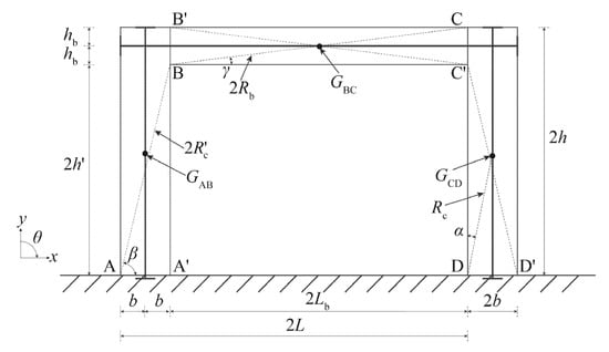
Figure 1.
Rigid body model of prestressed concrete rocking frame (PCRF).
The motion law of the PCRF is the same as that for the planar four-bar linkage mechanism shown in Figure 2, Figure 3 and Figure 4 when the PCRF is rocking. The rigid body model of the PCRF is a single degree of freedom system and can be described by a generalized coordinate. The rocking mechanism and planar four-bar linkage mechanism of the PCRF during counterclockwise rotation are shown in Figure 2. The dotted lines in Figure 1 and Figure 2 are used to illustrate the four-bar mechanism presented in Figure 3 and Figure 4. Hence, the planar four-bar linkage model can be used to obtain the relationship between the angles of the beam and columns. That is, the motion of the columns and beam when the PCRF is rocking can be represented by the motion of the bars in the four-bar linkage model. The governing equation of motion of the PCRF can be derived by the Lagrangian equation method. The angles of rotation of bars AB, BC and CD are denoted as , and , respectively. Figure 4 illustrates the planar four-bar model for the case and the case . The angle is positive and is negative in the case , while the opposite is positive for the case .
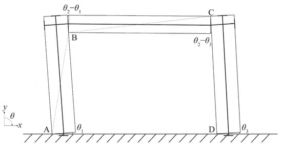
Figure 2.
Rocking mechanism and planar four-bar linkage mechanism of PCRF during counterclockwise rotation.
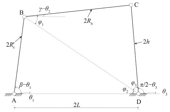
Figure 3.
Geometrical relationship of planar four-bar linkage mechanism for .
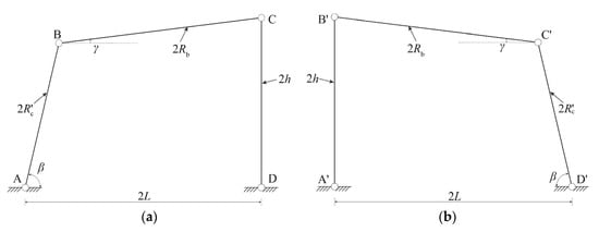
Figure 4.
Planar four-bar linkage mechanism of PCRF: (a) ; (b) .
3. Kinematics of the PCRF
The geometrical relationship of the planar four-bar linkage mechanism for is shown in Figure 3. Firstly, is assumed as a known angle, and are calculation auxiliary angles. From the geometry relationships, we have
The equations below can be obtained from sine and cosine law:
The expressions for and can be derived from Equations (1)–(5). The expressions are written as
Substituting Equation (2) into Equations (6) and (7) yields
Differentiating Equations (8) and (9) with respect to time , the corresponding angular velocities can be obtained and expressed for simplicity as
where is the angular velocity of bar AB and the upper dot denotes differentiation with respect to time . The symbol denotes a partial derivative with respect to . Similarly, the second partial derivatives of and with respect to can be written as
If point A is the coordinate origin, the positions after the deformation of the left column mass center , beam mass center and right column mass center are
4. Rocking Motion Equation
The governing equation of motion of the PCRF can be derived from the Lagrangian equation:
where T and V are the kinetic energy and potential energy of the PCRF. If the mass of the tendons is neglected, the potential energy of the PCRF can be calculated by
where is the gravitational potential energy of frame members, and is the elastic potential energy due to the elongation of tendons. If AD is regarded as the zero potential energy surface, then is expressed as
During rocking motion, the elastic potential energy can be derived as
The additional elongation of the tendon at the base of the left column can be obtained from the cosine law and the geometry relationship shown in Figure 5. We have
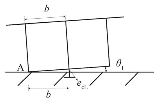
Figure 5.
The additional elongation of the tendon at the base of the left column.
Then the expression of can be written as
Similarly, the additional elongation of the tendon at the right column base is
The additional elongation of the beam tendon can be derived from the cosine law and the geometry relationships shown in Figure 2:
The expression of can be rewritten as
For simplicity, the two column tendons have the same parameters. Assuming is the initial pretension force of the column tendons, the initial elongation of the column tendon is
where is the stiffness of the column tendon, is the Young’s modulus of the tendon and is the cross-section area of the column tendons. Assuming is the initial pretension force of the beam tendon, the initial elongation of the beam tendon is
where is stiffness of the beam tendon and is the cross-section area of the beam tendon.
The kinetic energy of the PCRF can be calculated by Equation (24):
where is the velocity of the beam mass center. is the mass moment of inertia of the column with respect to the pivot point A or D. is the mass moment of inertia of the beam with respect to its mass center. The expression of can derived from Equation (25):
where is the velocity along the x-axis of the beam mass center. is the velocity along the y-axis of the beam mass center. Substituting Equation (25) into Equation (24) yields the kinetic energy of the PCRF:
During an admissible rotation , Equation (27) can be derived by the principle of virtual work
The virtual work caused by the external field forces is
where
Substituting Equations (28) and (29) into Equation (27) yields the generalized force :
The substitution of Equations (15), (16), (26) and (30) into Equation (13) results in the motion equation of the PCRF:
The terms , , , and in Equation (31) are nonlinear functions of the generalized coordinate and are expressed as Equation (32):
By considering the inherent symmetry of the PCRF, the motion equation of the PCRF for can be written in the same form as Equation (31), while the expressions of , , , and in this case are instead
The simplified and conservative starting condition for the calculation program can be obtained by ignoring the influence of the prestressing force on the triggering-off condition of the rocking motion for the PCRF. With this assumption, the lower bound solution of the minimum ground acceleration that initiates the rocking motion of the frame can be derived by substituting the initial conditions , and into Equation (31):
The calculation of can be obtained based on the expression of and in Equation (32) or Equation (33):
5. Calculation of Collision Energy Dissipation
It is assumed that energy dissipation occurs only during the collisions when the PCRF is rocking, that is, there is no energy consumption in the process of rotation. Considering that the duration of impact is extremely short, it can be assumed that the PCRF is always in a horizontal state during impacts. Collisions occur at the column feet and the inner faces at the beam-column joint in the case of a one-story single-span PCRF. Regardless of the plastic deformation of the tendons, the elongation of the tendons at the moment of collision is the initial elongation. The forces in the tendons are constant during the collision, which will not affect the momentum moments of the PCRF before and after the collision. The following assumptions are introduced to simplify the analysis and calculation of the collision energy dissipation of the PCRF. It is assumed that the collision forces on each collision surface concentrate on one point which is the postimpact rotation point of the identical rigid body. Relative slips between rigid members on each collision surface are not allowed. Non-collision forces such as gravity and the inertial force of members can be ignored compared to the collision force.
The case is taken as an example for analysis. The collision analysis model of the PCRF is shown in Figure 6 and the frame has returned to a zero-rotation state at this time. It is assumed that the angular velocity just before the collision is known of the frame column represented by bar AB. There are five unknowns: impulse and at collision point A’, and at collision point D’ and the postimpact angular velocity of the frame column represented by bar C’D’. The impulse at an arbitrary collision point i is defined as
where is the impact force and is the duration of impact. The ratio of angular velocity after and before the collision is defined as the coefficient of restitution . The solution of simultaneous Equations (37)–(41), which are derived in the following, returns the coefficient of restitution .
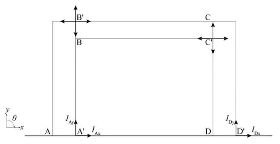
Figure 6.
Collision energy dissipation of PCRF for .
- Linear momentum conservation along the x-axis for the whole frame
- Linear momentum conservation along the y-axis for the whole frame
- Conservation of moment of momentum about point A′ for the whole frame
- Conservation of moment of momentum about point B′ for the left column
- Conservation of moment of momentum about point C′ for the right columnwhere is the moment of inertia of the column with respect to its mass center. The calculated expression for the coefficient of restitution is shown aswhere
The dimensionless parameters in Equation (43) are the mass ratio of beam to column , span-height ratio and height coefficient for the beam and for the column.
6. Time History Analysis of Seismic Response of the PCRF
The seismic response analysis of the PCRF is based on a basic model. The sections of the beam and columns are square. The frame is in the zero-rotation state without initial angular velocity and angular acceleration. The parameters of the basic model are shown in Table 1.

Table 1.
Parameters of the basic model.
The term ρc is the density of concrete, and the fracture elongation of the tendons is taken as 1%. The set of earthquake motion records recommended by the ATC-63 project [21] is selected as the source of earthquake records. The information of the earthquakes is shown in Table 2. Records ER1 to ER11 are far-field earthquakes, records ER12 to ER18 are pulse near-field earthquakes and the rest are no-pulse near-field earthquakes. The values of the peak ground acceleration (PGA) and peak ground velocity (PGV) of each earthquake record are also shown in Table 2.
Table 2.
Earthquake records.
According to the calculation results, the time of the rocking motion triggering-off, the time of peak ground acceleration (PGA), the maximum rotation and its occurrence time , as well as the maximum angular velocity and its occurrence time , can be obtained as shown in Table 3, where the maximum values of rotation and angular velocity are given in absolute values without the consideration of direction.
Table 3.
Time history analysis results of seismic response.
The result of ER15 is illustrated here to explain the characteristics of the seismic response of the PCRF. The time history curve of ER15 is shown in Figure 7 and the calculation results are presented in Figure 8. As shown in Figure 8a,b, does not exactly coincide with and . After the appearance of PGA and local maximum values of acceleration, the amplitudes of responses decay rapidly. At a time around 10.5 s, the frame motion approached the high-frequency vibration stage, in which the vibration amplitude is small and the peak of angular velocity is basically stable. It can be observed from Figure 8c,d that the phase orbit finally formed a spindle-shaped limit cycle which was centered on the origin in the phase diagram. The energy dissipation in the collisions of the PCRF is continuously supplied by the earthquake. Although the frame vibration in the high-frequency vibration stage is similar to steady-state vibration, it is named pseudo-steady-state vibration, considering that its external excitation is a random earthquake. It can be seen that the influence of external excitation on the frame motion is weakened significantly during this pseudo-steady-state vibration.
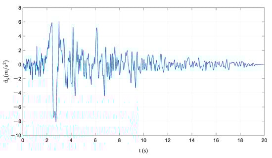
Figure 7.
Time history of earthquake record ER15.
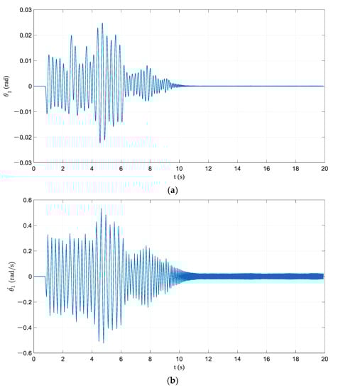
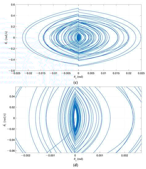
Figure 8.
Calculation results of basic frame model under ER15: (a) time history of rocking rotation; (b) time history of angular velocity; (c) phase orbit; (d) limit cycle.
In order to investigate the relationship between the key time points , , and of the basic model under different earthquakes, the of each response are all set as 1 s. The corresponding unified key time points can be obtained. The unified key time points of far-field and near-field earthquake records are shown in Figure 9 and Figure 10, respectively.
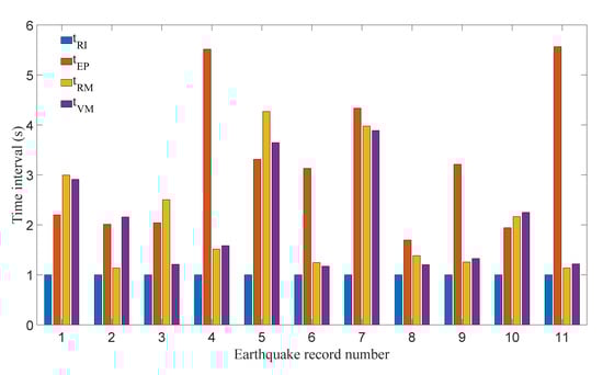
Figure 9.
Unified key time points in the case of far-field earthquakes.
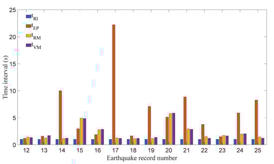
Figure 10.
Unified key time points in the case of near-field earthquakes.
Figure 9 illustrates that, under the far-field earthquakes, is very close to and they generally occur shortly after or near . In most of the cases that and appeared shortly after , the frame vibration has entered the pseudo-steady-state vibration stage or a stage with very small amplitudes of responses before . The amplification effect of PGA on frame response is no longer significant in this situation. When the time interval between and is small, the peak values of frame response appear around , or the , and are in close proximity to and , respectively. Figure 10 suggests that the difference between and is very small when the earthquakes are near-field earthquakes and they appear around or simultaneously. It can be found that the relationships between , , and are strongly dependent on the specific earthquake. The variety of earthquakes should be considered in the analysis of the PCRF.
The maximum elongations of prestressed tendons can be calculated based on the maximum rotation of the PCRF, as shown in Figure 11. It can be observed from Figure 11 that the maximum elongations of prestressed tendons are less than 0.5%, which have a large surplus from the 1% value of the fracture elongation of prestressed tendons. That is to say, the reserve of deformation capacity is sufficient and the seismic performance of the PCRF is prominent. It is worth emphasizing that the member connections of the PCRF proposed in this study depend mainly on the prestressed tendons and prestressing forces. Therefore, the structure failure of the PCRF will be led by the fracture of the prestressed tendons. Special attention should be given to the calculation of the deformation and elongation of prestressed tendons in analysis and design.
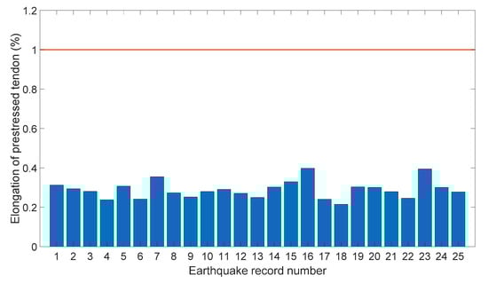
Figure 11.
Maximum elongations of prestressed tendons.
7. Parameter Analysis of PCRF Seismic Response
Eight independent dimensionless parameters can be proposed naturally during the derivation of the motion equation of the PCRF, which are the mass ratio of beam to column , span-height ratio , column aspect ratio , height coefficient , initial prestressing force of beam tendon , initial prestressing force of column tendon , linear stiffness of beam tendon and linear stiffness of column tendon . These are kept because any reduction of independent dimensionless parameters will inevitably influence the precision of the analysis in consideration of the nonlinearity of the rocking motion for the PCRF. The values of the dimensionless parameters for the basic frame model are , , , , , , and . Earthquake record ER15 is used as a test record and a parameter analysis of the PCRF seismic response is conducted.
A frame with a larger has a smaller response in the early stage of vibration, as shown in Figure 12. However, the responses of the frame are changed dramatically with the emergence of a large acceleration pulse at 2~3 s. In the meantime, the frame with a larger has a significantly larger angle and angular velocity compared with the smaller ones. A number of acceleration pulses appeared around 4 s, which increase the responses of the frame with further. The other frames have a smaller rotation before encountering multiple acceleration pulses and the amplification effect of multiple acceleration pulses on their response is limited. Different frames with different got into the pseudo-steady-state vibration eventually, while the frames with smaller entered earlier.
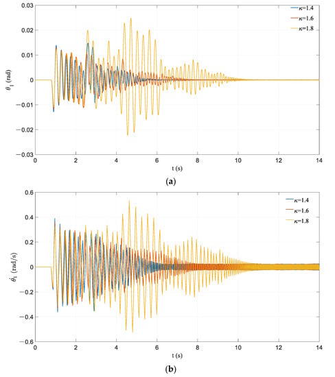
Figure 12.
Effect of variation in : (a) time history of rocking rotation; (b) time history of angular velocity.
The excessive increase in the response for the frame with caused by the first large acceleration pulse is counterintuitive. The mechanism of this phenomenon can be explained by the frame with larger having greater inertia force and energy after the acceleration pulse, causing a sudden increase in its response. The subsequent multiple acceleration pulses made the system response increase further. This phenomenon can be considered to suggest that the acceleration pulse has amplitude sensitivity to the amplification effect of the response of the PCRF. That is, when the vibration amplitude of the frame is large enough or greater than a threshold, the acceleration pulse has an amplification effect on the system response similar to resonance. The magnification of the system response increases with the enlargement of the system amplitude.
For further study of the influence of and the influence of earthquake characteristics, the far-field earthquake record of the Northridge earthquake in 1994, named ER2, is selected for analysis. The time history curve of ER2 and similar calculation results are illustrated in Figure 13. It can be seen that the frame with larger had a smaller vibration response in the whole vibration process and entered into pseudo-steady-state vibration earlier. Based on the above analysis, cases of different ground motion types should be fully considered in the analysis of PCRFs and time history analysis of various earthquake records is necessary.
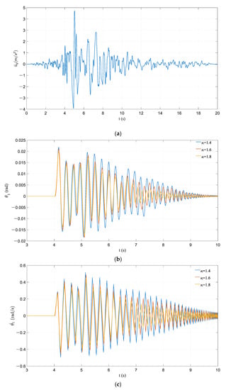
Figure 13.
Effect of variation in for the case of ER2: (a) time history of earthquake record ER2; (b) time history of rocking rotation; (c) time history of angular velocity.
It can be found in Figure 14 that the responses of frames with different are substantially close at the initial stage of vibration and the differences between responses are not changed significantly with the increase in vibration duration. When multiple consecutive acceleration pulses occurred, the response of the frame with smaller is obviously reduced, but the response of the frame with larger is increased significantly. Frames with different have different amplitudes when multiple continuous acceleration pulses are input. The accumulation of response amplification caused by acceleration pulses results in a large difference in subsequent calculation results. Parameter is a constant when is variational so the inertia forces of beam and columns are consistent in the analysis for . The variation range of is not very large in the research. It is for the above reasons that the influence of on the dynamic response of the PCRF is not similar to .
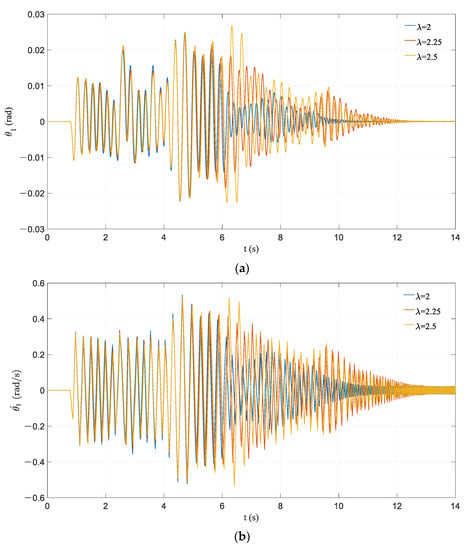
Figure 14.
Effect of variation in λ: (a) time history of rocking rotation; (b) time history of angular velocity.
As shown in Figure 15, the frames with different have different values of motion triggering-off time, which signifies that the frame with a larger column aspect ratio is more likely to be excited. A frame with a smaller column aspect ratio tends to stop at a faster speed. After the occurrence of multiple continuous acceleration pulses, the response of the frame with has a very obvious amplification effect. The response of the frame with , which entered the state of pseudo-steady-state vibration, hardly fluctuates.
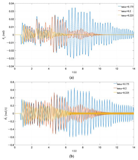
Figure 15.
Effect of variation in tanα: (a) time history of rocking rotation; (b) time history of angular velocity.
Figure 16 illustrates that the frame with a larger tends to become motionless faster than the smaller ones. When the first acceleration pulse is imported, it can be clearly seen that the response amplification of the frame with small amplitude is apparently weaker than that of the other frames. The acceleration pulse basically has no response amplification effect on the frame which is in the state of pseudo-steady-state vibration before the appearance of the acceleration pulse. The response of the frame with has a very obvious amplification phenomenon.
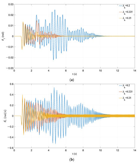
Figure 16.
Effect of variation in λh: (a) time history of rocking rotation; (b) time history of angular velocity.
It can be seen from the time history curves in Figure 17, Figure 18, Figure 19 and Figure 20 that the influence of dimensionless parameters related to prestressed tendons and initial prestressing forces on the frame responses are relatively consistent. The increase in dimensionless parameters can reduce the historical maximum responses of the frame markedly, which also leads to the earlier appearance of pseudo-steady-state vibration. The difference is that the influences on the vibration response in the initial stage are miscellaneous. A frame with a large initial prestressing force has a relatively large response at the initial stage of vibration, while the cases of the linear stiffness of prestressed tendons are the opposite.
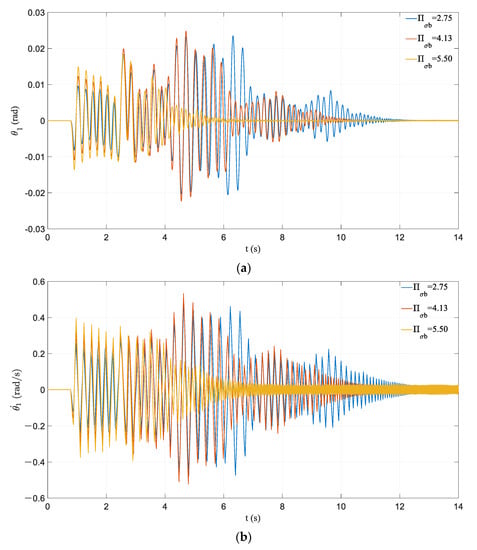
Figure 17.
Effect of variation in : (a) time history of rocking rotation; (b) time history of angular velocity.
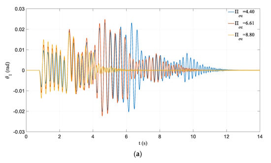
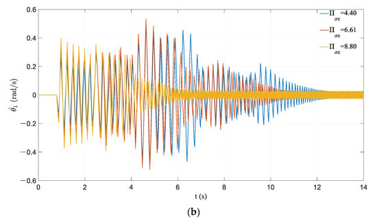
Figure 18.
Effect of variation in : (a) time history of rocking rotation; (b) time history of angular velocity.
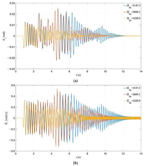
Figure 19.
Effect of variation in : (a) time history of rocking rotation; (b) time history of angular velocity.
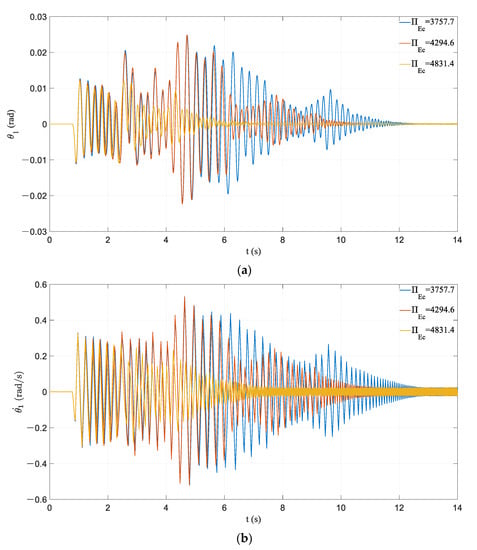
Figure 20.
Effect of variation in : (a) time history of rocking rotation; (b) time history of angular velocity.
8. Conclusions
The theoretical model based on rigid body of a one-story single-span PCRF is established. The corresponding governing motion equation of the PCRF is derived based on the model and the numerical solution of the motion equation is obtained. The energy dissipation of the PCRF is analyzed and the calculation method for the coefficient of restitution is proposed. Time history analyses of the seismic response of the PCRF are carried out with different types of earthquake records. The analysis results show that the maximum rotation of the frame is small and the capacity of structural deformation is sufficient, which means the PCRF has promising seismic performance. The member connections of the PCRF proposed in this study depend on the prestressed tendons and prestressing forces. The structure failure of the PCRF will be led by the fracture of prestressed tendons so the calculation of the deformation and elongation of prestressed tendons should be cautious in analysis and design.
A pseudo-steady-state vibration of the PCRF may appear after some duration of vibration under earthquake excitation, in which case a steady spindle-shaped limit cycle is finally formed by phase orbit in the phase diagram. The influence of external excitation on the vibration of the PCRF is weakened significantly in the state of pseudo-steady-state vibration. The parameter analysis of the PCRF is conducted based on eight dimensionless parameters. The results reveal the characteristic influences of the dimensionless parameters on the seismic response of the PCRF. The parameters related to prestressed tendons and initial prestressing forces have a consistent influence on the seismic response of the PCRF, and maximum values of seismic response decrease with the increase in the respective parameters. The influences of dimensionless parameters of mass and geometry on the seismic response of the PCRF are complicated, in which case the type of earthquake also needs to be considered. It is worth noting that when the rotational earthquake component and the translational earthquake component are considered simultaneously in the analysis, the motion of the rocking frame will be a three-dimensional motion. The influence of the rotational earthquake component on the seismic response of the PCRF needs further research.
Author Contributions
Conceptualization, X.S. and Z.Z.; methodology, Z.Z. and X.S.; software, Z.Z.; validation, X.S. and Z.Z.; formal analysis, Z.Z.; investigation, Z.Z. and X.S.; resources, X.S.; data curation, Z.Z.; writing—original draft preparation, Z.Z.; writing—review and editing, X.S. and Z.Z.; visualization, Z.Z.; supervision, X.S.; project administration, X.S.; funding acquisition, X.S. Both authors have read and agreed to the published version of the manuscript.
Funding
This research was funded by National Natural Science Foundation of China (NSFC) (Grant No. 51178328).
Institutional Review Board Statement
Not applicable.
Informed Consent Statement
Informed consent was obtained from all subjects involved in the study.
Data Availability Statement
The data presented in this study are available on request from the corresponding author.
Conflicts of Interest
The authors declare no conflict of interest.
References
- Housner, G.W. Limit Design of Structures to Resist Earthquakes. In Proceedings of the First World Conference on Earthquake Engineering, Berkeley, CA, USA, 1 January 1956; pp. 5-1–5-11. [Google Scholar]
- Housner, G.W. The Behavior of inverted pendulum structures during earthquakes. Bull. Seismol. Soc. Am. 1963, 53, 403–417. [Google Scholar]
- Pacific Earthquake Engineering Research Center. Report of the Seventh Joint Planning Meeting of NEES/E-Defense Collaborative Research on Earthquake Engineering; PEER Report 2010/109; University of California, Berkeley: Berkeley, CA, USA, 2010. [Google Scholar]
- Mitsumasa, M.; Tatsuya, A.; Tadashi, I.; Yutaka, M.; Yoshiyuki, M.; Akira, W. Earthquake response reduction of buildings by rocking structural systems. In Proceedings of the Smart Structures and Materials 2002: Smart Systems for Bridges, Structures, and Highways, San Diego, CA, USA, 28 June 2002; pp. 265–272. [Google Scholar]
- Roh, H.; Reinhorn, A.M. Nonlinear Static Analysis of Structures with Rocking Columns. J. Struct. Eng. 2010, 136, 532–542. [Google Scholar] [CrossRef]
- Hitaka, T.; Sakino, K. Cyclic Tests on a Hybrid Coupled Wall Utilizing a Rocking Mechanism. Earthq. Eng. Struct. Dyn. 2008, 37, 1657–1676. [Google Scholar] [CrossRef]
- Kibriya, L.T.; Málaga-Chuquitaype, C.; Kashani, M.M.; Alexander, N.A. Nonlinear dynamics of self-centring rocking steel frames using finite element models. Soil Dyn. Earthq. Eng. 2018, 115, 826–837. [Google Scholar] [CrossRef]
- Wada, A.; Qu, Z.; Motoyui, S.; Sakata, H. Seismic retrofit of existing SRC frames using rocking walls and steel dampers. Front. Archit. Civ. Eng. China 2011, 5, 259–266. [Google Scholar] [CrossRef]
- Makris, N.; Vassiliou, M.F. Planar rocking response and stability analysis of an array of free-standing columns capped with a freely supported rigid beam. Earthq. Eng. Struct. Dyn. 2013, 42, 431–449. [Google Scholar] [CrossRef]
- Dimitrakopoulos, E.G.; Giouvanidis, A.I. Seismic response analysis of the planar rocking frame. J. Eng. Mech. 2015, 141, 04015003. [Google Scholar] [CrossRef]
- Vassiliou, M.F.; Mackie, K.R.; Stojadinovic, B. A finite element model for seismic response analysis of deformable rocking frames. Earthq. Eng. Struct. Dyn. 2017, 46, 447–466. [Google Scholar] [CrossRef]
- Priestley, M.J.N.; Tao, J.R. Seismic Response of Precast Prestressed Concrete Frames with Partially Debonded Tendons. PCI J. 1993, 38, 58–69. [Google Scholar] [CrossRef]
- Cheok, G.; Lew, H. Model Precast Concrete Beam-to-column Connections Subject to Cyclic Loading. PCI J. 1993, 38, 80–92. [Google Scholar] [CrossRef]
- Priestley, M.J.N.; MacRae, G.A. Seismic Tests of Precast Beam-to-column Joint Subassemblages with Unbounded Tendons. PCI J. 1996, 41, 64–81. [Google Scholar] [CrossRef]
- El-Sheikh, M.T.; Sause, R.; Pessiki, S.; Lu, L. Seismic Behavior and Design of Unbonded Post-Tensioned Precast Concrete Frames. PCI J. 1999, 44, 54–71. [Google Scholar] [CrossRef]
- Makris, N.; Vassiliou, M.F. Dynamics of the Rocking Frame with Vertical Restrainers. J. Struct. Eng. 2014, 141, 04014245. [Google Scholar] [CrossRef]
- Giouvanidis, A.I.; Dimitrakopoulos, E.G. Seismic performance of rocking frames with flag-shaped hysteretic behavior. J. Eng. Mech. 2017, 143, 04017008. [Google Scholar] [CrossRef]
- Lu, L.; Liu, X.; Chen, J.; Lu, X. Seismic performance of a controlled rocking reinforced concrete frame. Adv. Struct. Eng. 2017, 20, 4–17. [Google Scholar] [CrossRef]
- Song, L.; Guo, T.; Chen, C. Experimental and numerical study of a self-centering prestressed concrete moment resisting frame connection with bolted web friction devices. Earthq. Eng. Struct. Dyn. 2014, 43, 529–545. [Google Scholar] [CrossRef]
- Guo, T.; Song, L.; Cao, Z.; Gu, Y. Large-Scale Tests on Cyclic Behavior of Self-Centering Prestressed Concrete Frames. ACI Struct. J. 2016, 113, 1263–1274. [Google Scholar] [CrossRef]
- Applied Technology Council, Federal Emergency Management Agency. Quantification of Building Seismic Performance Factors; FEMA P695; Federal Emergency Management Agency: Washington, DC, USA, 2009. [Google Scholar]


Publisher’s Note: MDPI stays neutral with regard to jurisdictional claims in published maps and institutional affiliations. |
© 2021 by the authors. Licensee MDPI, Basel, Switzerland. This article is an open access article distributed under the terms and conditions of the Creative Commons Attribution (CC BY) license (http://creativecommons.org/licenses/by/4.0/).