Abstract
Biomedical engineers prefer decision forests over traditional decision trees to design state-of-the-art Parkinson’s Detection Systems (PDS) on massive acoustic signal data. However, the challenges that the researchers are facing with decision forests is identifying the minimum number of decision trees required to achieve maximum detection accuracy with the lowest error rate. This article examines two recent decision forest algorithms Systematically Developed Forest (SysFor), and Decision Forest by Penalizing Attributes (ForestPA) along with the popular Random Forest to design three distinct Parkinson’s detection schemes with optimum number of decision trees. The proposed approach undertakes minimum number of decision trees to achieve maximum detection accuracy. The training and testing samples and the density of trees in the forest are kept dynamic and incremental to achieve the decision forests with maximum capability for detecting Parkinson’s Disease (PD). The incremental tree densities with dynamic training and testing of decision forests proved to be a better approach for detection of PD. The proposed approaches are examined along with other state-of-the-art classifiers including the modern deep learning techniques to observe the detection capability. The article also provides a guideline to generate ideal training and testing split of two modern acoustic datasets of Parkinson’s and control subjects donated by the Department of Neurology in Cerrahpaşa, Istanbul and Departamento de Matemáticas, Universidad de Extremadura, Cáceres, Spain. Among the three proposed detection schemes the Forest by Penalizing Attributes (ForestPA) proved to be a promising Parkinson’s disease detector with a little number of decision trees in the forest to score the highest detection accuracy of 94.12% to 95.00%.
1. Introduction
Parkinson’s Disease (PD) is a neurodegenerative disorder that is mostly reported in older adults. It is a late age disease having no visible symptoms at its early stage. This is one of the major problems found in the aged person due to the disorder of neuro-related functions in the brain after Alzheimer [1,2]. In 2015, a study about all-cause mortality revealed more than 177,000 death cases around the globe due to Parkinson’s disease [3]. The reason behind the significant casualty of Parkinson’s is due to the lack of concrete diagnostical remedy. Parkinson’s disease happened as a result loss of dopaminergic neurons in the substantia nigra as the age progresses. Hence, one of the best options left with the clinical practitioners to delay the speed of dopamine loss. Therefore, it is essential to detect and diagnose the disease at an early stage.
The Electroencephalogram (EEG) signal [4], gait [5,6,7,8], acoustic signal [9,10,11], Magnetic Resonance Imaging (MRI) [12], and handwriting signals [13,14,15] are mostly used by the researchers to detect the presence of Parkinson’s disease. Out of various options to detect Parkinson’s, the acoustic signal of voice plays a prominent role in the early detection of the disease. It is because the vocal impairment is found from the beginning of the disease and even years before a clinical diagnosis can be made [16,17,18,19].
There exist many state-of-the-art machine learning approaches to detect the presence of PD at the initial stage [20,21,22]. Most of the modern machine learning techniques employ decision trees and few handfuls of approaches rely on decision forests. Though the decision trees proved to be efficient classifying acoustic voice signal data, at the same time decision forests are preferable over traditional decision trees as decision forests are more precise, accurate and able to handle overfitting and underfitting situations smartly through decision tree ensemble. Random Forest, as a random tree ensemble frequently used for Parkinson’s detection [23,24], relies on bagging approach of ensemble, which makes the decision forest versatile [25]. However, Random Forest [26] is not the only decision forest that exists in the literature. There are two recently devised approaches in data science, i.e., Systematically Developed Forests (SysFor) [27] and Forest by Penalizing Attributes (ForestPA) [28]. Many literatures suggest that the SysFor, and ForestPA are equally versatile as Random Forest. However, there is a need of describing the efficiency of decision forests in terms of tree density in the forest and a dynamic training, and testing split. In this article, three distinct Parkinson’s detection schemes have been proposed using Random Forest, SysFor, and ForestPA. The proposed schemes undertake varying tree density with incremental training and testing samples to detect the presence of Parkinson’s. The detection capability of decision forests is measured with the lowest number of decision trees they form during the process of classification to achieve maximum detection efficiency.
A challenge lies in data science, especially in medical datasets is about the ideal training and testing split of underlying data. The ideal training and testing split are still debatable. Many articles related to Parkinson Detection carried out the evaluation using 60–40% splitting of training and testing sets, whereas many others claim the 80–20% is ideal. In view of this contradiction, this article finds a suitable training and testing instances split of acoustic signal data for Parkinson’s detection. Another challenge that the Parkinson detection approaches face while using acoustic signal is a selection of prominent voice-based features. In other words, the acoustic signal contains many voice-based features. For instance, baseline features of voice signal consist of Pitch period entropy (PPE) and Detrended fluctuation analysis (DFA) and various jitter, shimmer and Harmonic to Noise Ration attributes of the voice signal. Similarly, time frequency features comprise of Intensity parameters, Formant frequency and Bandwidth. Intensity represents the loudness of speech signal which is related to the subglottis pressure of the airflow that depends on the tension and vibration of the vocal folds [9,29]. On the other hand, many derived voice-based feature segments are realized, viz., Mel-Frequency Cepstral Coefficients (MFCC) [30,31], Wavelet [32] and Tunable Q-Factor wavelet transform (TQWT) [9] respectively for identification Parkinson’s disease. These features are extracted from the acoustic signal using specialized software. Therefore, in this context, while analyzing decision forests algorithms an effort has been made to identification of the suitable feature segment that promotes detection accuracy of Parkinson’s detection.
The contribution of this article is as follows:
- Development of three distinct Parkinson’s detection systems using three supervised decision forest algorithms, viz., SysFor, ForestPA and Random Forest.
- Identifying the lowest number of trees required to achieve maximum detection rate in the decision forests.
- Identification of the ideal training and testing split of the acoustic signal data of Parkinson’s and control subjects has also been carried out for achieving maximum performance.
- A detailed investigation has also been carried out to identify the ideal feature segments of the acoustic signals for effective detection of Parkinson.
Rest of the article is as follows. Section 2 deals with various literatures of Parkinson’s Disease Detection (PDD) using decision forest algorithms. Decision forest algorithms used in this article are detailed in Section 3. Section 4 discusses materials and methods towards the aims and objectives of this article. Section 5 deals with results and discussion followed by conclusion at Section 6 of this article.
2. Literature Review
The literature has been reviewed in two broad areas. At first, various articles are reviewed explaining state-of-the-art decision forest algorithms proposed in the field of data science. Second, few promising articles related to decision forests algorithms used for Parkinson’s disease detection has been discussed.
Decision forests have been proposed by many researchers and widely used due to the ability to achieve maximum predictability of incoming instances. Leo Breiman [26] introduced the first version of Random Forest as a decision forest algorithm. Random Forests undertakes bagging as the training method on Random Subspace. For a set of features f the size of features chosen randomly for training purposes are , where m is the number of inputs [25]. The benefit of Random Forest is its versatility to varying data size. However, the major drawback of Random Forest lies with the number of trees that it employs for classifying data. However, Random Forest employs a significant number of trees for effective training and classification of incoming instances. At the same time, with the increase in number of trees the time complexity of Random Forest is also increases [33].
There are many variations of Random Forest [34,35,36,37,38,39] are proposed so far. Cutler & Zaho [40] proposed a perfect random tree ensemble, where the attribute behind the splitting criteria is chosen randomly. Cascading and Sharing Trees, a decision forest algorithm ranks the features according to their contribution towards the classification. The gain ratio scores are allocated to the attributes for ranking. At the post ranking phase, the attribute having the highest gain ratio score has been taken as root node. The second tree of the forest is the attribute having the second-highest gain ratio score. Tripoliti et al. [41] proposed a dynamic growing of trees in Random Forest. The dynamic tree growth is determined by polynomial fit function, where the best fit has been achieved through root mean squared error. Their approach reveals detection accuracy of 74.60% to 87.5% with 32 to 72 trees in the forest. In a similar structure, Adnan et al. [42] proposed an ensemble pruning method using genetic algorithm to overcome demerits of huge number of decision trees involved in decision forest building process. The ensemble pruning method not only computationally efficient but also shows better ensemble accuracy. Similarly, Kushwah et al. [43] combined input output paradigm of neural network with Random Forest ensemble for classification of gene expression data, where members of the ensemble were selected from the set of neural network classifiers. Though, their approach magnificently classifies gene expression data, but the approach is silent about the decision forest building procedure. On the other hand, their approach presents classification performance in terms of ratio of class percentage. Maximally Diversified Multiple Decision Tree (MDMDT) [44], a decision forest was proposed, where each tree tests a new attribute from the dataset. The training process of the MDMDT tree is like the generalized decision tree. However, during the testing phase, the non-key attributes tested by the first tree are removed and the second tree is trained on remaining attributes. These processes iteratively continue till all the defined number of trees in the forest are built. A decision forest known as Systematically Developed Forest of Multiple Decision Trees (SysFor) has been proposed where the number of trees is defined before the forest building process [27]. The number of good attributes is ascertained based on the goodness threshold defined by the user. Similarly, the split points are determined based on the separation threshold defined by the user. The user intervention makes the forest build controlled and more tolerant to overfitting. A decision forest known as Extremely Randomized Tree (ERT) has been proposed, where cut-points for numerical attributes are chosen randomly. ERT has been proposed to build on the training samples rather than bootstrap samples. However, another decision forest called Forest by Penalizing Attributes (ForestPA) Decision Forest uses bootstrap samples to build the forest. After generating samples, ForestPA selects the splitting attribute for a node using a merit value of the attribute. The merit value of attributes is dynamic and is computed by multiplying the classification capacity with the current weight of the attribute. The default weight for each attribute is initialized to 1.0 while building the first decision tree in the forest. The weights are kept on changing during the tree building process.
Machine Learning (ML) proved to be a great tool in many fields of medical science [41,42,43,44,45,46,47,48,49] including but not limited to Parkinson’s Detection [50,51,52,53,54,55,56,57]. For Parkinson’s Disease Detection (PDD) Random Forest as a decision forest algorithm is used in combination with other promising preprocessing algorithms. For instance, Smekal et al. [54] proposed a PD detection technique using a combination of Random Forest and Mann-Whitney U test algorithm to predict Parkinson. Their approach reveals an impressive accuracy of 84.96%, sensitivity of 84.52% and specificity of 85.71%. Random Forest is also used along with Principal Component Analysis (PCA) for segregation of PD from control subjects [24]. The features generated by PCA boost the detection accuracy by up to 96.83%. This is due to the little number of features results in the formation of adequate trees for prediction. Sakar et al. [9] compared many supervised classification techniques along with Random Forest on acoustic signals to predict Parkinson. The research reveals that the Random Forest impressively detects the presence of Parkinson’s disease from the bandwidth, formant frequencies, intensity, and vocal-based features. Polat et al. [23] proposed a PD detection model using Random Forest and Synthetic Minority Over-sampling Technique (SMOTE). The tree formation realizes a detection accuracy of 94.89%. Similarly, an automated detection of Parkinson’s disease based on Minimum Average Maximum Tree (MAMT) been proposed for Parkinson’s detection [55]. The MAMT approach took the help of singular value decomposition method to achieve a superb detection accuracy of 92.46%. Further, boosting approaches such as XGBoost [56] and Gaussian Mixture Model (GMM) [57] proved to be a reliable Parkinson’s detection approach. These boosting models not only efficiently detect the presence of Parkinson but also found to be precise in the detection process.
3. Decision Forests
The proposed work in this article illuminates newly proposed decision forests namely SysFor, ForestPA and the most popular, Random Forest. Here we described the chosen algorithms and highlighting their main features and working procedure.
3.1. Random Forest (RF)
In the year 2001, the Random Forest algorithm has been proposed as a robust decision forest by Leo Breiman [26]. Since then, Random Forest attracted more than 63,000 citations in various areas of data science. The power of Random Forest lies with the way of establishing decision trees in the forests with a set of bootstrap samples. For a dataset of dimensions, a random variable is a set of input variables (also known as predictor variables) and is a real values response variable, where RF deduce a prediction function for correctly predicting . During the prediction process the lowest error represented by a loss function determines the closeness of with . RF also has provision to penalizes for strong deviation from .
Random Forest has been designed to address both classification and regression problems. However, in line with the aim and objectives of this article the analysis has been restricted to the classification only. Therefore, from the classification point of view, the loss function is the zero-one loss and is represented as:
In other words, the classification function for each response values of can be represented as:
which is nothing but the Bayes rule. Equation (2) determines the classification approach for single decision tree. However, for number of decision trees (), the classification function of Random Forest is:
Here, is the indicator function. It should be noted that the RF relies on the principle of recursive binary partitioning [58,59,60,61]. The predictor space used to be partitioned on individual variable of . Concerning the classification, the splitting criteria for each nonterminal node is calculated through the Gini index and mathematically represented as:
where, = Number of classes, = Contributed proportion of class in the node The node can be estimated as:
Cutler et al. [58] derived Random Forest both for classification and regression. As the classification is the purpose of this research work, Equations (1)–(5) has been referred in the context of classification.
During the splitting process, two child nodes are created on the left and right side which is further subjected to splitting like parent node. The process repeated tilling the terminal nodes are achieved (on stopping criteria). Each of the terminal nodes comes up with a predicted result. The predicted result at the terminal nodes for each observation is the maximum repeating class for that observation, which is nothing but the predicted class for concern observation. This principle is applicable to continuous variables. However, for categorical attributes, the final class is decided upon the voting of the prediction result of decision trees.
3.2. Systematicaly Developed Forest (SysFor)
Another vibrant decision forest called Systematically Developed Forest of Multiple Decision Tree (SysFor) has been proposed recently by Islam et al. [27]. Instead of adopting all variables, SysFor considers only the variables having highest contribution towards the classification process; thus, drastically improving the speed of classification. Another strength of this decision forest algorithm is its ability to build trees even from datasets having low dimensions. The SysFor works on two distinct phases. The first step involves selection of potential attributes and the second stage involves building the forest through decision trees using the potential attributes. The famous C4.5 decision tree has been incorporated as ensemble within the forest.
3.2.1. Identification of Potential Attributes
The potential feature identification process starts with scanning the features of the dataset say . The process also additionally accepts user defined threshold points, i.e., a threshold for choosing the potential attributes, also known as goodness threshold (), and a threshold for feature separation (). Both these threshold points are responsible for a clear-cut distinction between potential and non-potential attributes. The gain-ratio of attributes plays a crucial role for identifying potential attributes. Both the numerical and categorical attributes are treated differently while evaluating gain-ratio; thus, making the entire process robust and scalable. At first, the whole non-class attributes are scanned one by one. For categorical attributes, the attribute itself and its gain ratio are added to two distinct sets separately & , where is the attribute sets and represents the set of gain ratio. Similarly, the numerical splitting point for attributes is kept reserved to a negative number in a separate set . In this case, the authors in [27] uses as the splitting point. It is because unlike numerical attributes the categorical attribute does not have a splitting point. Similarly, for numerical attributes, the splitting point is determined by maintaining the following relation for all other available splitting point (:
where, is any available splitting points and is the splitting point in P. After estimating all the splitting points, the split point having the highest gain ratio is added to the set and . The process of adding gain ratio and corresponding splitting point continues till a single splitting point realized. It is because the size of is inversely proportional to available splitting points. Finally, the attribute positions are sorted in the descending order of gain ratio, which gives an opportunity to select the potential attributes. The attributes having the gain ratio below the goodness threshold are selected for building the C4.5 decision trees and SysFor decision forest.
3.2.2. Building the Decision Forest
Once the number of good attributes is in hand, the SysFor decision forest is built upon, which proved to be fast and more accurate in the classification process. Based on the descending order of gain ratio score, the attributes are picked up one by one to build the C4.5 trees in the SysFor decision forests. If the attribute is categorical, the underlying data is partitioned based on unique values (categories) of that attribute. On the other hand, for numerical attributes the dataset is partitioned into two horizontal segments based on the split points achieved for these attributes. Finally, C4.5 decision trees are created as ensemble on those partitions. For a set of data segments , if and represents the number of instances and good attributes of segments, respectively, the number of trees in the forest can be estimated as:
Using the prediction results of T number of trees in the forest, SysFor applies the voting scheme to reach the final decision about the unlabeled incoming instances.
3.3. Decision Forest by Penalizing Attributes (ForestPA)
Another novel decision forest called Decision Forest by Penalizing Attributes (ForestPA) [28] has been proposed by the same authors of SysFor with a provision for penalizing attributes during the tree building process. Unlike SysFor, which plants C4.5 decision trees in the forest, the ForestPA plants the Classification and Regress Tree (CART) as an effective decision-maker. Like Random Forest, the ForestPA generates a bootstrap sample from the original training instances . The CART decision trees are built upon these samples, where the attributes merit values decide the splitting point. The merit values of an attribute is calculated as:
where represents the classification capacity and represents weights of attribute A. The first tree is generated with the default weight 1. The weight of the attributes is gradually increased during the tree building process. The level of the tree decides the final weight of the attributes. A weight range function of for tree level of decreases the attribute weight and is represented as:
The Equation (9) essentially allocates advantageous weight to the lower level nodes & penalizes to the higher-level nodes. In the other words, the nodes having lower rules in hand have more advantageous weight & nodes having significant values have disadvantageous weights. Moreover, there are incidents where an attribute is tested at the root node, thus, scoring the lowest weight of 0.0000, which results the attribute not to be selected in subsequent trees. Therefore, the authors suggested a dynamic increase in weight on the attributes that are tested at the root node only. The weight increment value of such attributes is calculated as:
where is the weight of the attribute obtained from a tree at level and is the height of the tree (highest level in the tree). The process of dynamic allocation of weight allows the decision trees to predict the unlabeled instances. The prediction output of the trees is combined and the final decision about the class label of the instance is determined through voting.
4. Materials and Methods
For Parkinson’s detection, two modern datasets of Parkinson’s and control subjects have been used. The first dataset for the proposed detection approach has been provided by the Department of Neurology in Cerrahpaşa, Faculty of Medicine, Istanbul (hereafter Istanbul acoustic dataset) in the year 2019 [9]. The dataset is recent and gaining popularity due to the significant number of participants and a wide array of acoustic features. The dataset contains acoustic features of 252 subjects, out of which 64 are controls (33 men and 41 women) and 188 subjects (107 men and 81 women) suffering from PD. The age group found in the dataset are 33 to 87. During the data collection process, the microphone is set to 44.1 KHz. The sound files were used to generate various primary and derived features. Each feature segment contains multiple features, which constitutes a total of 754 features. The characteristics of the various features segments is presented in Table 1.

Table 1.
General structure of Istanbul acoustic dataset.
The dataset contains three primary feature segments and three derived feature segments. Generally, primary features are most frequently used and recognized by the technicians engaged in PD diagnosis. The primary feature segments extracted are Baseline, Time Frequency and Vocal Fold. Similarly, the derived feature segments are Mel-Frequency Cepstral Coefficients (MFCC), Wavelet and Tunable Q-Factor wavelet transform (TQWT) respectively. These features are extracted from the acoustic signal using specialized software. Both the Primary and derived features are used for analysis in this article. The dataset is class-imbalanced due to a higher number of PD subjects.
Another acoustic dataset considered here is donated by Departamento de Matemáticas, Universidad de Extremadura, Cáceres, Spain (Spanish acoustic dataset) [62,63]. The dataset Contains acoustic features extracted from 3 voice recordings of the sustained/a/phonation of 80 subjects. The dataset is perfectly balanced with 40 of them diagnosed with Parkinson’s and 40 controls. The dataset contains 40 attributes pertaining to Jitter, Shimmer, MFCCs, etc.
The acoustic features analysis through decision forests has been conducted in two stages. At first, three decision forest algorithms Random Forest, SysFor and ForestPA has been subjected for comparison along with six state-of-the-art supervised classifiers, viz., k-Nearest Neighbor (kNN), C4.5, Logistic Regression, Back-Propagation Neural Network (BPNN), Naïve Bayes and OneR. The classifiers are used to classify each feature segment stated in Table 1. The identification features are dropped from the dataset as these features are no direct link with the primary and derived features. The 10-fold cross-validation approach has been used to validate the performance of the classifiers. The validation process applied to each feature segment separately on primary and derived feature segments. This will also help to identify the prominent feature segments’ contribution towards the Parkinson’s detection.
There exist many performance measures for decision forests, viz., detection accuracy, mis classification rate, precision, false alarm rate. Specifically, for Random Forest, test error is estimated based on out-of-bag error as Random Forest works on bootstrap sampling. According to a recent study by Janitza et al. [64], the OOB revealed overestimated in balanced settings and in settings with few samples. In our case the dataset has only 252 instances and the training and testing split of instances are selected ranging from 30–70% to 80–20%. In the case of bootstrap sample by Random Forest, the size of training set may be reduced further, which may seriously impact OOB error estimates. Therefore, other performance measures like detection accuracy, precision has been considered for evaluating decision forests as Parkinson’s detector. Moreover, since two more decision forests ForestPA and SysFor has been taken into consideration; the accuracy measure has been given preference over error based on OOB. The detection accuracy of decision forests has been estimated for comparison and analysis is presented below.
where TP = True Positive instances, TN = True Negative instances, FP = False Positive instances and FN = False Negative instances.
The output of the classifiers of each feature segment is presented in Table 2.
Table 2.
The detection accuracy of supervised classifiers on each feature segments of Istanbul acoustic dataset.
Classifying each feature segment shows satisfying detection accuracy for all classifiers. However, for a specific feature segment, a specific classifier shows highest accuracy rate. For an instance, the Random Forest shows better classification accuracy for Time Frequency, MFCC and TQWT feature segments. Similarly, the Baseline and Wavelet features are classified nicely by BPNN and OneR, respectively. On the other hand, using the vocal fold features, the SysFor decision forest segregates PD subjects from controls with 79.37% accuracy. It is evident that decision forests, viz., Random Forest and SysFor are responsible for the best acquired result for almost all feature segments due to the ensemble of decision trees in the forest. However, it does not imply that the decision forests are the best option as compared to other supervised classification techniques. Therefore, to come across a valid conclusion, the primary features viz. time frequency, baseline and vocal folds and the derived features, viz., MFCC, TQWT and wavelets are merged separately. The merged feature segments are again subjected to classification. Table 3 shows the performance of classifiers on the primary and derived features segments independently along with all feature segments.
Table 3.
The detection accuracy of supervised classifiers on primary and derived features of Istanbul acoustic dataset.
By merging the similar feature segments together, it is observed that the decision forests, viz., Random Forest, SysFor and ForestPA shows distinct and the better result both in primary and derived features. Not only that, the decision forests also show best accuracy rate by merging and classifying combined primary and derived features. Though it is clearly visible that the decision forests are far better approach for Parkinson’s detection, yet it is difficult to identify the best decision forests among three. In one hand, the SysFor shows better result for primary and derived features but for the entire feature segments with 752 features the ForestPA classifier outperforms other decision forests. This is the reason for which a second stage test is essential to identify the most suitable decision forest along with an ideal acoustic feature segment.
At the second stage of analysis and training and testing split on dataset has been conducted. Instead of a traditional way of splitting the underlying data into training and testing groups, a dynamic way of training and testing instances split has been conducted. Moreover, the performance of the decision forests is also observed with different tree sizes in the forest. This second stage analysis, which is the theme of this article has been presented in Figure 1.
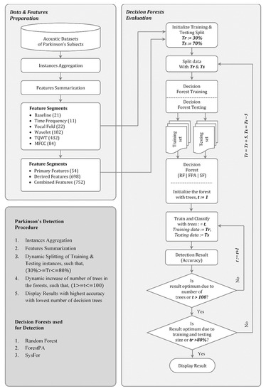
Figure 1.
The proposed decision forest based Parkinson’s detection.
From the literature review, it is revealed that most of the modern PD detection techniques rely on Random Forest as a base learner. However, it is also observed from Table 3 that both the SysFor and ForestPA are a better choice than the Random Forest. According to Sinnott et al., (2016) [33] and Oshiro et al. [65], the performance of Random forest decreases with the additional deployment of number of trees in the forest beyond the required numbers. The performance of Random Forest always increases up to a certain number of trees [33]. Afterwards, the deployment of additional trees only increases the computational cost of the classification process [65]. Therefore, controlling the number of decision trees in the forest would improve the time complexity of the entire testing and training process with realization of optimum detection accuracy. In this section, an effort has been made to identify the minimum number of trees required to achieve highest detection accuracy. Instead of leaving the decision forests by their own, the number of tree formation is controlled in each iteration of training and test process. This process continues till the maximum accuracy has been realized with the formation of minimum number of trees. In the meantime, the process will also suggest the ideal training and testing instance split for a dataset. The algorithm for the identifications of perfect training and testing instance split and minimum number of trees required to achieve highest performance output has been outlined in Table 4.
Table 4.
The process of decision forests based Parkinson’s detection.
The process starts with initially splitting the data as 30% training and 70% testing. It has been observed that there is no clear-cut guideline regarding training and testing instance split. Researchers decide the training testing split according to their implementation environment and convenience [7,66,67]. On the other hand, machine learning tools like WEKA states default training testing instance split as 66%–34% [68,69]. In the absence of a concrete guideline, a loop has been created with training size of 30% and testing size of 70% to training size of 80% and testing size of 20%. In each iteration, the percentage of training size has been incremented by 5%. In each iteration of the training-testing split, the number of trees deployed has been changed from the 1 to a maximum number of trees to 100. This will give us an unbiased analysis of the decision forest for knowing the exact number of trees required to get the highest detection accuracy with the lowest number of errors. However, the main reason for setting the tree limits in the forest up to 100 is that the decision forests have different tree formation limitations. For instance, the SysFor classifier has the default number of trees is 60, whereas the ForestPA decision forest deploys 10 trees by default. Similarly, the Random Forest supports a maximum of 100 decision trees by default [68,69]. Moreover, according to Sinnott et al. [33] 100 trees are sufficient in the case of Random Forest for achieving the desired stopping criteria.
It should be noted that decision forest like Random Forest randomly selects bootstrap samples for train decision trees. On the other hand, bootstrap sampling is not a cure for small dataset. Therefore, with the increase in training instances, the power of Random Forest increases. This is the reason; we have dynamically increasing the training size from 30% to 80%. This will ensure to identify the size of training set to get the maximum detection accuracy. Similarly, with the increase in number of decision trees in the forest, the detection power of the forest improved. This ensures to get highest detection result at certain point of time having reasonably smaller number of trees in hand.
5. Results and Discussion
From the 10-fold cross-validation the result was not determined to get the best decision forest and the best feature segment for Parkinson’s detection. Therefore, a dynamic training and testing split of instances with change in number of trees has been carried out and, in the meanwhile, three distinct Parkinson’s detection schemes has also been proposed using decision forests. The result of the proposed approaches has been obtained in two different ways. At first, the detection accuracy of decision forests has been observed with a change in the number of decision trees for each block of the training-testing split. Secondly, the best training-testing split has been proposed as the PDS with the smallest number of decision tree formation for getting the highest detection accuracy with lowest error rate. The analysis has been conducted on both the acoustic signal datasets mentioned in Section 4.
The performance of decision forests with incremental number of decision trees and training testing splits on Istanbul acoustic signal dataset are outlined in Figure 2. At each change in training and testing split and number of decision trees, the performance of decision forests varies. From Figure 2, it is observed that the ForestPA and SysFor require lesser number of trees to achieve highest accuracy. With just 30% of training instances, both ForestPA and SysFor show the detection accuracy between 80%–90%. However, with the increase in number of trees the Random Forest shows the superior result than its peer. A similar result is observed with 40% training instances. However, with increase in training instances the SysFor evolves as a leading decision forest with very little number of trees. With 60% training instances the SysFor infers a visible performance improvement over other decision forests. It should be noted that all the decision forests do not require a significant number of trees to touch the highest accuracy mark. Therefore, during the classification process, the number of trees in the forests should be controlled rather than leaving it to the environment.
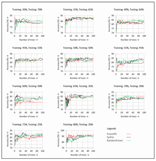
Figure 2.
Detection accuracy with respect to change in number of trees in the decision forests observed for each training and testing split on Istanbul acoustic dataset.
A similar kind of observation is also noticed for the Spanish acoustic dataset presented in Figure 3. Figure 3 shows the detection accuracy derived from the decision forest with a change in trees for various training and testing split. It can be seen from the figure that, both the ForestPA and SysFor shows better detection accuracy for each increase in tree size. The highest detection accuracy is also observed within just 20 decision trees. This shows the default number of decision trees for SysFor is not reliable. With only below 10 decision trees, the SysFor shows better results for all training and testing split in terms of detection accuracy.
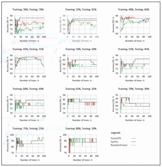
Figure 3.
Detection accuracy with respect to change in number of trees in the decision forests observed for each training and testing split on Spanish acoustic dataset.
Further, the 75–25% training and testing split reveal the highest detection accuracy for all the decision forest. Though SysFor seems to be ahead of ForestPA and Random Forest for almost all the training-testing split, all the decision forest reveals the highest accuracy for 75–25% split.
To come across a concrete conclusion, the decision forests are further analyzed for the highest detection accuracy with minimum number of trees (t), precision (Prc), sensitivity (Sen), specificity (Spc), fall-out, and miss rate. The result obtained by second level of analysis for all the decision forests has been presented in Table 5, Table 6 and Table 7.
Table 5.
Maximum performance received for SysFor classifier with minimum number of decision trees on primary and derived features of Istanbul acoustic dataset.
Table 6.
Maximum performance received for Random Forest classifier with minimum number of decision trees on primary and derived features of Istanbul acoustic dataset.
Table 7.
Maximum performance received for ForestPA classifier with minimum number of decision trees on primary and derived features of Istanbul acoustic dataset.
Table 5, Table 6 and Table 7 does not really compare the decision forests algorithms, instead, it shows the performance of the decision forests on various feature segments of acoustic datasets provided by the Department of Neurology in Cerrahpaşa, Istanbul. However, the performance comparison of the classifier can be analyzed for each feature segment. The column “t” indicates the minimum number of decision trees deployed to achieve such maximum performances. Similarly, the number of features for each feature segment is denoted by “m”. Overall, the performance of the decision forests presented in Table 5, Table 6 and Table 7 is far better than the performance of the same decision forests (with the default number of trees) outlined in Table 2 and Table 3. For an instance, the detection accuracy observed by SysFor, Random Forest and ForestPA received are 82.54%, 88.24%, and 86.28% with the help of 7, 4, and 69 decision trees in the forests, respectively, which is 1.98%, 13.64%, and 8.5% higher than the decision forests deployed in its default setting. Moreover, the SysFor classifier gains the peak detection accuracy with 50% training instances only. The same implication can be observed for all feature segments. Therefore, it is evident that the dynamic allocation of decision trees shows far better results than the default number of decision trees. Since the focusing point is to present three Parkinson detection systems using the decision forests, it is essential to compare the performance of decision forests to understand the versatility of the forests towards Parkinson’s detection. In this context, three popular performance measures, viz., detection accuracy, sensitivity and specificity utilized for better analysis of the decision forests. The detection accuracy, sensitivity and specificity of decision forests for all feature segments are shown in Figure 4, Figure 5 and Figure 6, respectively.
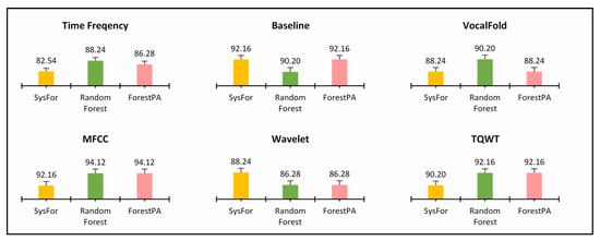
Figure 4.
Highest detection accuracy of decision forest algorithms with minimum number of trees on various feature of Istanbul acoustic dataset.
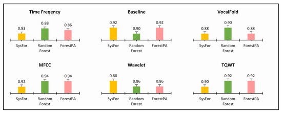
Figure 5.
Highest sensitivity of decision forest algorithms with minimum number of trees on various feature of Istanbul acoustic dataset.
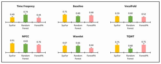
Figure 6.
Highest specificity of decision forest algorithms with minimum number of trees on various feature of Istanbul acoustic signal dataset.
Figure 4 shows mixed results for all the decision forests. For Time Frequency, Vocal Fold, and MFCC, the Random Forest shows best detection rate. Similarly, SysFor shows better results for Wavelet feature segments. Not only this, the ForestPA revealed at par result than its peer forests in Baseline and TQWT features.
Similarly, in Figure 5 also all the classifiers have identical sensitivity; thus, an inconclusive result about the best decision forest. Both Random Forest and ForestPA have equal sensitivity for MFCC and TQWT derived features and SysFor and ForestPA have equal sensitivity rate for Baseline and VocalFold Features.
On the other hand, the SysFor outperforms other decision forests in Baseline, MFCC, and Wavelet feature segments, whereas Random Forests performs well with highest sensitivity in time frequency, Vocal Fold feature segment. Though an indication has been received that the SysFor would be a good approach towards Parkinson’s detection with better sensitivity than its peers, more conclusive evidence is expected to justify the claim. Therefore, at the next step the combined primary feature segments (Time Frequency, Baseline and Vocal Fold) and combined derived feature segments (MFCC, TQWT and Wavelet) and the total feature segments are treated separately with the decision forests. The result of decision forests on respective combined feature segments and total feature segments are presented in Table 8, Table 9 and Table 10.
Table 8.
Maximum performance received for decision forests with minimum number of decision trees on primary feature segments of Istanbul acoustic dataset.
Table 9.
Maximum performance received for decision forests with minimum number of decision trees on derived feature segments of Istanbul acoustic dataset.
Table 10.
Maximum performance received for decision forests with minimum number of decision trees on all feature segments of Istanbul acoustic dataset.
From Table 8 the Random Forest shows highest accuracy of 92.16% for primary feature segment. However, does merely acquiring the highest accuracy make the Random Forest winner? It is because Random Forest achieves such performance with 17 decision trees, which is much more than that of its peers. On the other hand, the SysFor decision forest took only three trees to yields an impressive accuracy of 90.20%. Not only that, the SysFor also reveals magnificent lowest fall-out and highest miss-rate while segregating Parkinson’s subjects from control subjects. This is what the medical practitioners are looking for. It is because an ideal Parkinson’s detection system should not classify a control subject as Parkinson and vice versa. Another reason for which the SysFor can be considered as an ideal Parkinson detector is the specificity. With 82.50% specificity, the SysFor classifies control subjects perfectly.
Similarly, for derived feature segments, ForestPA reckons the highest ever performance with just nine trees in the forest. Not only that, the ForestPA performs well in precision, sensitivity, fall-out and miss-rate. However, it slips away in specificity.
Finally, when all the feature segments are combined and processed through decision forests separately, the ForestPA still retains its position with 94.12% of detection accuracy. The ForestPA also reveals the best result in all performance measures, viz., accuracy, precision, sensitivity, specificity, fall-out and miss-rate.
At this point, it is quite clear that the ForestPA is the ideal decision forest for acoustic signal-based Parkinson’s detection, but comparing Table 8 and Table 9 analogically it is quite evident that the primary feature segments such as time frequency, baseline and vocal fold are the better segment as compared to derived features. With better precision and specificity with lowest fall-out and miss rate the primary feature segments contribute better towards the Parkinson’s detection process. Nevertheless, ForestPA proved to be a decent Parkinson’s detector with better results in derived features but, at the same time, it also took only seven trees in the case of primary features with satisfactory detection results. Therefore, in a nutshell the primary feature segments are proved to be better features as compared to derived features.
At this point it is proved that the proposed approach for decision forest based Parkinson’s detection shows convincing results when decision trees are controlled within the forest. However, it is quite interesting to observe the potentiality of the proposed approach with the recent state of the art approaches. In this regard few recent Parkinson’s detection approach has been shortlisted and compared. The approaches used for comparison are the deep learning based Convolutional Neural Networks (CNN) Parkinson’s detection [52], Random Forest and SMOTE hybrid [23], Minimum Average Maximum Tree (MAMT) approach [55], XGBoost approach [56] and Gaussian Mixture Models (GMM) approach [57]. All these approaches are based on the same dataset and on same evaluation criteria. The comparative analysis has been presented in Table 11.
Table 11.
Comparative analysis of the proposed ForestPA approach of Parkinson’s detection with other cutting-edge approaches of Istanbul acoustic dataset.
From the Table 11 it can be observed that our proposed approach with ForestPA controlled decision trees dynamically proved to be superior Parkinson’s detector as compared to other detection scheme. The nine layer of CNN deep learning approach [52] though shows promising result, but the method is not convincing even at per with other machine learning approaches. It is because, the dataset size is limited to only few subjects and the deep learning approaches which are designed for data sensitive applications are unable to gather required classification information from such small samples. The CNN based deep learning approach founds to be a better choice than XGBoost approach [56] with a 2.10% higher detection accuracy. The proposed ForestPA approach also shows better classification accuracy as compared to MAMT [55] and Random Forest and SMOTE combination approaches. The artificial samples generated by SMOTE and classified by Random Forest does not even stand tall in front of ForestPA approaches. Our approach reveals 1.78% more detection accuracy than Random Forest and SMOTE combination. However, to achieve such detection accuracy our detection approach took 698–752 acoustic features. Therefore, in a landscape, controlling the decision trees in ForestPA has been proved to enhance better detection accuracy.
Finally, the decision forests are proposed as an ideal Parkinson’s detector by controlling the decision trees in the forest. To ensure the stability and robustness of the proposed approach further, the Spain acoustic signal dataset has been incorporated for Parkinson’s detection. The Spain acoustic signal dataset also reveals similar results for all the three decision forests are presented in Table 12.
Table 12.
Maximum performance received for decision forests with minimum number of decision trees on all feature segments of Spanish acoustic dataset.
According to Table 12, all the three-decision forest shows satisfying performance. Nevertheless, the Random Forest achieves equal accuracy rate at par with ForestPA and SysFor but it is unable to win the race due to other performance measures like precision, sensitivity, and specificity. Overall, the ForestPA evolves as the best decision forest having equal detection result along with its peers having only decision tree in the forest. Incremental decision trees in ForestPA no doubt proved to be a great approach for optimum classification. However, it is not essentially the best approach in its class. Therefore, from the functional point of view, it is essential to compare our approach with the approaches having similar functionalities. This will help us to understand the efficiency of the approaches proposed in similar guidelines. In this regard approaches like Tripoliti et al. [41], Adnan et al. [42] has been selected for comparison keeping in mind the similar structure and guideline as per the proposed approach. Table 13 represents the comparison of the ensemble approaches having similar structures and guidelines.
Table 13.
Comparison of the proposed approach with other state of the approaches having similar functionality and guidelines.
From Table 13, it can be observed that the proposed approach shows better classification accuracy as compared to similar state of the art approaches. The Random Forest approach shows better average detection accuracy along with SysFor and ForestPA incremental decision forest approach. The datasets used by Tripoliti et al. [41] and Adnan et al. [42] are different than the datasets we considered. Nevertheless, keeping in view the similar growing structures the GRF [41] and SubPGA [42] expected to perform better for variety of dataset. Tripoliti et al. [41] also admitted the same fact that their approach exhibits well in 90% of test cases. However, in the case of other 10% test cases the approach of Tripoliti et al. [41] appears to be struggling; thus, conclude with lower average accuracy score. On the other hand, the incremental Random Forest approach shows highest accuracy of 93.58.
6. Conclusions
In this article, two recently proposed decision forests namely SysFor and ForestPA along with most popular Random Forest has been used as Parkinson’s detectors. As a novel contribution in the field of Parkinson’s detection, the proposed Parkinson’s detection method employs incremental decision trees and training instances. At each iteration of the proposed method, the number of decision trees has been increased withing a range of 1 to 100 and the training instances has been increases from 30% to 80%. The threshold point having maximum detection accuracy has been identified and the iterative method has been presented as a potential Parkinson detector. The proposed methods have been tested on two recent acoustic datasets of Parkinson’s and control subjects. It is found that the proposed method on ForestPA decision forest holds only nine decision trees in the forest to achieve maximum detection accuracy of 94.12% with nine decision on the Istanbul acoustic dataset. Similarly, for the Spanish acoustic dataset, ForestPA shows 95% accuracy with just one decision tree in the forest. Moreover, the average detection accuracy has been ascertained for both the acoustics datasets under study. The average detection accuracy on incremental trees of Random Forest Random forest shows 93.58% of detection accuracy, which is a better choice than the SysFor and ForestPA approach. However, it is suggested that, while choosing the right approach for Parkinson’s detection, the underlying feature segments and number of features therein should be taken into consideration. It is worth to mention that the primary feature segments, viz., time frequency, vocal fold and baseline features are the better choice than derived feature segments for incremental decision forests. The proposed method has also been compared with existing state-of-the-art Parkinson’s detection and other medical disease detection approaches. The comparative analysis reveals that the proposed method of incremental decision trees in the forest detect the Parkinson’s subject more efficiently than the counterparts. In the future, various feature selection schemes can be incorporated with decision forests for improving the performance of the decision forests further.
Author Contributions
M.P., R.P., P.N., A.K.B. and P.B. have designed the study, developed the methodology, performed the analysis, and written the manuscript. All authors have read and agreed to the published version of the manuscript.
Funding
This research received no external funding.
Institutional Review Board Statement
We choose to exclude this statement as the study did not require ethical approval.
Informed Consent Statement
“Not applicable” for studies not involving humans.
Data Availability Statement
Data available in a publicly accessible repository (UCI Machine Learning Repository) that does not issue DOIs.
Conflicts of Interest
The authors declare no conflict of interest.
References
- Dlay, J.K.; Duncan, G.W.; Khoo, T.K.; Williams-Gray, C.H.; Breen, D.P.; Barker, R.A.; Burn, D.J.; Lawson, R.A.; Yarnall, A.J. Progression of Neuropsychiatric Symptoms over Time in an Incident Parkinson’s Disease Cohort (ICICLE-PD). Brain Sci. 2020, 10, 78. [Google Scholar] [CrossRef] [PubMed]
- Lyketsos, C.G.; Carrillo, M.C.; Ryan, J.M.; Khachaturian, A.S.; Trzepacz, P.; Amatniek, J.; Cedarbaum, J.; Brashear, R.; Miller, D.S. Neuropsychiatric symptoms in Alzheimer’s disease. Alzheimer’s Dement. 2011, 7, 532–539. [Google Scholar] [CrossRef] [PubMed]
- Wang, H.; Naghavi, M.; Allen, C.; Barber, R.M.; Bhutta, Z.A.; Casey, D.C.; Charlson, F.J.; Chen, A.Z.; Coates, M.M.; Coggeshall, M.; et al. Global, regional, and national life expectancy, all-cause mortality, and cause-specific mortality for 249 causes of death, 1980–2015: A systematic analysis for the Global Burden of Disease Study 2015. Lancet 2016, 388, 1459–1544. [Google Scholar] [CrossRef]
- Yuvaraj, R.; Murugappan, M.; Acharya, U.R.; Adeli, H.; Ibrahim, N.M.; Mesquita, E. Brain functional connectivity patterns for emotional state classification in Parkinson’s disease patients without dementia. Behav. Brain Res. 2016, 298, 248–260. [Google Scholar] [CrossRef]
- Joshi, D.; Khajuria, A.; Joshi, P. An automatic non-invasive method for Parkinson’s disease classification. Comput. Methods Programs Biomed. 2017, 145, 135–145. [Google Scholar] [CrossRef]
- Zeng, W.; Liu, F.; Wang, Q.; Wang, Y.; Ma, L.; Zhang, Y. Parkinson’s disease classification using gait analysis via deterministic learning. Neurosci. Lett. 2016, 633, 268–278. [Google Scholar] [CrossRef]
- Alkhatib, R.; Diab, M.O.; Corbier, C.; El Badaoui, M. Machine Learning Algorithm for Gait Analysis and Classification on Early Detection of Parkinson. IEEE Sens. Lett. 2020, 4, 1–4. [Google Scholar] [CrossRef]
- Mikos, V.; Heng, C.-H.; Tay, A.; Yen, S.-C.; Chia, N.S.Y.; Koh, K.M.L.; Tan, D.M.L.; Au, W.L. A Wearable, Patient-Adaptive Freezing of Gait Detection System for Biofeedback Cueing in Parkinson’s Disease. IEEE Trans. Biomed. Circuits Syst. 2019, 13, 503–515. [Google Scholar] [CrossRef]
- Sakar, C.O.; Serbes, G.; Gündüz, A.; Tunc, H.C.; Nizam, H.; Sakar, B.E.; Tutuncu, M.; Aydin, T.; Isenkul, M.E.; Apaydin, H. A comparative analysis of speech signal processing algorithms for Parkinson’s disease classification and the use of the tunable Q-factor wavelet transform. Appl. Soft Comput. 2019, 74, 255–263. [Google Scholar] [CrossRef]
- Mostafa, S.A.; Mustapha, A.; Mohammed, M.A.; Hamed, R.I.; Arunkumar, N.; Ghani, M.K.A.; Jaber, M.M.; Khaleefah, S.H. Examining multiple feature evaluation and classification methods for improving the diagnosis of Parkinson’s disease. Cogn. Syst. Res. 2019, 54, 90–99. [Google Scholar] [CrossRef]
- Gottapu, R.D.; Dagli, C.H. Analysis of Parkinson’s disease data. Procedia Comput. Sci. 2018, 140, 334–341. [Google Scholar] [CrossRef]
- Cigdem, O.; Beheshti, I.; Demirel, H. Effects of different covariates and contrasts on classification of Parkinson’s disease using structural MRI. Comput. Biol. Med. 2018, 99, 173–181. [Google Scholar] [CrossRef] [PubMed]
- Afonso, L.C.; Rosa, G.H.; Pereira, C.R.; Weber, S.A.T.; Hook, C.; De Albuquerque, V.H.C.; Papa, J.P. A recurrence plot-based approach for Parkinson’s disease identification. Futur. Gener. Comput. Syst. 2019, 94, 282–292. [Google Scholar] [CrossRef]
- Rios-Urrego, C.D.; Vásquez-Correa, J.C.; Vargas-Bonilla, J.F.; Nöth, E.; Lopera, F.; Orozco-Arroyave, J.R. Analysis and evaluation of handwriting in patients with Parkinson’s disease using kinematic, geometrical, and non-linear features. Comput. Methods Programs Biomed. 2019, 173, 43–52. [Google Scholar] [CrossRef]
- Ali, L.; Zhu, C.; Golilarz, N.A.; Javeed, A.; Zhou, M.; Liu, Y. Reliable Parkinson’s Disease Detection by Analyzing Handwritten Drawings: Construction of an Unbiased Cascaded Learning System Based on Feature Selection and Adaptive Boosting Model. IEEE Access 2019, 7, 116480–116489. [Google Scholar] [CrossRef]
- Harel, B.; Cannizzaro, M.; Snyder, P.J. Variability in fundamental frequency during speech in prodromal and incipient Parkinson’s disease: A longitudinal case study. Brain Cogn. 2004, 56, 24–29. [Google Scholar] [CrossRef]
- Postuma, R.B.; Lang, A.E.; Gagnon, J.-F.; Pelletier, A.; Montplaisir, J.Y. How does parkinsonism start? Prodromal parkinsonism motor changes in idiopathic REM sleep behaviour disorder. Brain 2012, 135, 1860–1870. [Google Scholar] [CrossRef]
- Rusz, J.; Hlavnička, J.; Tykalová, T.; Bušková, J.; Ulmanová, O.; Růžička, E.; Sonka, K. Quantitative assessment of motor speech abnormalities in idiopathic rapid eye movement sleep behaviour disorder. Sleep Med. 2016, 19, 141–147. [Google Scholar] [CrossRef]
- Jeancolas, L.; Benali, H.; Benkelfat, B.-E.; Mangone, G.; Corvol, J.-C.; Vidailhet, M.; Lehericy, S.; Petrovska-Delacretaz, D. Automatic detection of early stages of Parkinson’s disease through acoustic voice analysis with mel-frequency cepstral coefficients. In Proceedings of the 2017 International Conference on Advanced Technologies for Signal and Image Processing (ATSIP), Fez, Morocco, 22–24 May 2017; pp. 1–6. [Google Scholar]
- Montaña, D.; Campos-Roca, Y.; Pérez, C.J. A Diadochokinesis-based expert system considering articulatory features of plosive consonants for early detection of Parkinson’s disease. Comput. Methods Programs Biomed. 2018, 154, 89–97. [Google Scholar] [CrossRef]
- Solana-Lavalle, G.; Galán-Hernández, J.-C.; Rosas-Romero, R. Automatic Parkinson disease detection at early stages as a pre-diagnosis tool by using classifiers and a small set of vocal features. Biocybern. Biomed. Eng. 2020, 40, 505–516. [Google Scholar] [CrossRef]
- Tracy, J.M.; Özkanca, Y.; Atkins, D.C.; Ghomi, R.H. Investigating voice as a biomarker: Deep phenotyping methods for early detection of Parkinson’s disease. J. Biomed. Informatics 2020, 104, 103362. [Google Scholar] [CrossRef] [PubMed]
- Polat, K. A hybrid approach to Parkinson disease classification using speech signal: The combination of SMOTE and random forests. In Proceedings of the 2019 Scientific Meeting on Electrical-Electronics & Biomedical Engineering and Computer Science (EBBT), Istanbul, Turkey, 24–26 April 2019. [Google Scholar] [CrossRef]
- Aich, S.; Younga, K.; Hui, K.L.; Al-Absi, A.A.; Sain, M. A nonlinear decision tree based classification approach to predict the Parkinson’s disease using different feature sets of voice data. In Proceedings of the 2018 20th International Conference on Advanced Communication Technology (ICACT), Chuncheon-si, Korea, 11–14 February 2018; pp. 638–642. [Google Scholar]
- Adnan, N. Decision Tree and Decision Forest Algorithms: On Improving Accuracy, Efficiency and Knowledge Discovery Clustering-Based Recommender System View Project. 2017. Available online: https://www.researchgate.net/publication/321474742 (accessed on 22 August 2020).
- Breiman, L. Random Forests. Mach. Learn. 2001, 45, 5–32. [Google Scholar] [CrossRef]
- Islam, Z.; Giggins, H. Knowledge Discovery through SysFor: A Systematically Developed Forest of Multiple Decision Trees Brand Switching in Mobile Phones and Telecommunications View Project A Hybrid Clustering Technique Combining a Novel Genetic Algorithm with K-Means View Project Knowledge Discovery through SysFor-a Systematically Developed Forest of Multiple Decision Trees. 2011. Available online: https://www.researchgate.net/publication/236894348 (accessed on 21 August 2020).
- Adnan, N.; Islam, Z. Forest PA: Constructing a decision forest by penalizing attributes used in previous trees. Expert Syst. Appl. 2017, 89, 389–403. [Google Scholar] [CrossRef]
- Mongia, P.K.; Sharma, R.K. Estimation and Statistical Analysis of Human Voice Parameters to Investigate the Influence of Psychological Stress and to Determine the Vocal Tract Transfer Function of an Individual. J. Comput. Netw. Commun. 2014, 2014, 1–17. [Google Scholar] [CrossRef]
- Gómez-Rodellar, A.; Álvarez-Marquina, A.; Mekyska, J.; Palacios-Alonso, D.; Meghraoui, D.; Gómez-Vilda, P. Performance of Articulation Kinetic Distributions Vs MFCCs in Parkinson’s Detection from Vowel Utterances. In Neural Approaches to Dynamics of Signal Exchanges; Springer: Singapore, 2020; pp. 431–441. [Google Scholar]
- Soumaya, Z.; Taoufiq, B.D.; Nsiri, B.; Abdelkrim, A. Diagnosis of Parkinson disease using the wavelet transform and MFCC and SVM classifier. In Proceedings of the 2019 4th World Conference on Complex Systems (WCCS), Ouarzazate, Morocco, 22–25 April 2019; pp. 1–6. [Google Scholar] [CrossRef]
- Drissi, T.B.; Zayrit, S.; Nsiri, B.; Ammoummou, A. Diagnosis of Parkinson’s Disease based on Wavelet Transform and Mel Frequency Cepstral Coefficients. Int. J. Adv. Comput. Sci. Appl. 2019, 10. [Google Scholar] [CrossRef]
- Sinnott, R.; Duan, H.; Sun, Y. A Case Study in Big Data Analytics: Exploring Twitter Sentiment Analysis and the Weather. In Big Data—Principles and Paradigms; Morgan Kaufmann: Burlington, MA, USA, 2016. [Google Scholar]
- Bernard, S.; Heutte, L.; Adam, S. Forest-RK: A new random forest induction method. Lect. Notes Comput. Sci. 2008, 5227, 430–437. [Google Scholar] [CrossRef]
- Bonissone, P.; Cadenas, J.M.; Garrido, M.C.; Díaz-Valladares, R.A. A fuzzy random forest. Int. J. Approx. Reason. 2010, 51, 729–747. [Google Scholar] [CrossRef]
- Bernard, S.; Adam, S.; Heutte, L. Dynamic Random Forests. Pattern Recognit. Lett. 2012, 33, 1580–1586. [Google Scholar] [CrossRef]
- Adnan, M.N. On dynamic selection of subspace for random forest. Lect. Notes Comput. Sci. 2014, 8933, 370–379. [Google Scholar] [CrossRef]
- Seyedhosseini, M.; Tasdizen, T. Disjunctive normal random forests. Pattern Recognit. 2015, 48, 976–983. [Google Scholar] [CrossRef]
- Blaser, R.; Fryzlewicz, P. Random Rotation Ensembles. J. Mach. Learn. Res. 2016. [Google Scholar] [CrossRef]
- Cutler, A.; Zhao, G. PERT-Perfect Random Tree Ensembles. 2001. Available online: https://www.researchgate.net/publication/268424569 (accessed on 21 August 2020).
- Tripoliti, E.E.; Fotiadis, D.I.; Manis, G. Automated Diagnosis of Diseases Based on Classification: Dynamic Determination of the Number of Trees in Random Forests Algorithm. IEEE Trans. Inf. Technol. Biomed. 2011, 16, 615–622. [Google Scholar] [CrossRef] [PubMed]
- Adnan, M.N.; Islam, M.Z. Optimizing the number of trees in a decision forest to discover a subforest with high ensemble accuracy using a genetic algorithm. Knowl. Based Syst. 2016, 110, 86–97. [Google Scholar] [CrossRef]
- Kushwah, J.; Singh, D. Classification of cancer gene selection using random forest and neural network based ensemble classifier. Int. J. Adv. Comput. Res. 2013, 3, 30. [Google Scholar]
- Hu, H.; Li, J.; Wang, H.; Daggard, G.; Shi, M. A Maximally Diversified Multiple Decision Tree Algorithm for Microarray Data Classification. Available online: http://www.cs.waikato.ac.nz/ml/weka/ (accessed on 21 August 2020).
- Mishra, S.; Tripathy, H.K.; Mallick, P.K.; Bhoi, A.K.; Barsocchi, P. EAGA-MLP—An Enhanced and Adaptive Hybrid Classification Model for Diabetes Diagnosis. Sensors 2020, 20, 4036. [Google Scholar] [CrossRef]
- Wernick, M.N.; Yang, Y.; Brankov, J.G.; Yourganov, G.; Strother, S.C. Machine Learning in Medical Imaging. IEEE Signal Process. Mag. 2010, 27, 25–38. [Google Scholar] [CrossRef]
- Reamaroon, N.; Sjoding, M.W.; Lin, K.; Iwashyna, T.J.; Najarian, K. Accounting for Label Uncertainty in Machine Learning for Detection of Acute Respiratory Distress Syndrome. IEEE J. Biomed. Heal. Inform. 2018, 23, 407–415. [Google Scholar] [CrossRef]
- Barsocchi, P. Position Recognition to Support Bedsores Prevention. IEEE J. Biomed. Heal. Inform. 2012, 17, 53–59. [Google Scholar] [CrossRef]
- Crivello, A.; Barsocchi, P.; Girolami, M.; Palumbo, F. The Meaning of Sleep Quality: A Survey of Available Technologies. IEEE Access 2019, 7, 167374–167390. [Google Scholar] [CrossRef]
- Bhoi, A.K. Classification and Clustering of Parkinson’s and Healthy Control Gait Dynamics Using LDA and K-means. Int. J. Bioautom. 2017, 21, 19–30. [Google Scholar]
- Wang, W.; Lee, J.; Harrou, F.; Sun, Y. Early Detection of Parkinson’s Disease Using Deep Learning and Machine Learning. IEEE Access 2020, 8, 147635–147646. [Google Scholar] [CrossRef]
- Gunduz, H. Deep Learning-Based Parkinson’s Disease Classification Using Vocal Feature Sets. IEEE Access 2019, 7, 115540–115551. [Google Scholar] [CrossRef]
- Ali, L.; Zhu, C.; Zhang, Z.; Liu, Y. Automated Detection of Parkinson’s Disease Based on Multiple Types of Sustained Phonations Using Linear Discriminant Analysis and Genetically Optimized Neural Network. IEEE J. Transl. Eng. Heal. Med. 2019, 7, 1–10. [Google Scholar] [CrossRef]
- Smekal, Z.; Mekyska, J.; Galaz, Z.; Mzourek, Z.; Rektorova, I.; Faundez-Zanuy, M. Analysis of phonation in patients with Parkinson’s disease using empirical mode decomposition. In Proceedings of the 2015 International Symposium on Signals, Circuits and Systems (ISSCS), Iasi, Romania, 9–10 July 2015; pp. 1–4. [Google Scholar]
- Tuncer, T.; Dogan, S.; Acharya, U.R. Automated detection of Parkinson’s disease using minimum average maximum tree and singular value decomposition method with vowels. Biocybern. Biomed. Eng. 2020, 40, 211–220. [Google Scholar] [CrossRef]
- Abdurrahman, G.; Sintawati, M. Implementation of xgboost for classification of parkinson’s disease. J. Physics: Conf. Ser. 2020, 1538, 012024. [Google Scholar] [CrossRef]
- Bchir, O. Parkinson’s Disease Classification using Gaussian Mixture Models with Relevance Feature Weights on Vocal Feature Sets. Int. J. Adv. Comput. Sci. Appl. 2020, 11. [Google Scholar] [CrossRef]
- Cutler, A.; Cutler, D.R.; Stevens, J.R. Random Forests. In Ensemble Machine Learning; Springer: Boston, MA, USA, 2012; pp. 157–175. [Google Scholar]
- Franklin, J. The elements of statistical learning: Data mining, inference and prediction. Math. Intell. 2005, 27, 83–85. [Google Scholar] [CrossRef]
- Izenman, A.J. Modern Multivariate Statistical Techniques; Springer: New York, NY, USA, 2008. [Google Scholar]
- Zhang, H.; Singer, B.H. Recursive Partitioning and Applications; Springer: New York, NY, USA, 2010. [Google Scholar]
- Naranjo, L.; Pérez, C.J.; Campos-Roca, Y.; Martín, J. Addressing voice recording replications for Parkinson’s disease detection. Expert Syst. Appl. 2016, 46, 286–292. [Google Scholar] [CrossRef]
- Naranjo, L.; Pérez, C.J.; Martín, J.; Campos-Roca, Y. A two-stage variable selection and classification approach for Parkinson’s disease detection by using voice recording replications. Comput. Methods Programs Biomed. 2017, 142, 147–156. [Google Scholar] [CrossRef]
- Janitza, S.; Hornung, R. On the overestimation of random forest’s out-of-bag error. PLoS ONE 2018, 13, e0201904. [Google Scholar] [CrossRef]
- Oshiro, T.M.; Perez, P.S.; Baranauskas, J.A. How many trees in a random forest? In Proceedings of the International Workshop on Machine Learning and Data Mining in Pattern Recognition, Berlin, Germany, 13–20 July 2012; pp. 154–168. [Google Scholar]
- Gemci, F.; Ibrikci, T. Using Deep Learning Algorithm to Diagnose Parkinson Disease with High Accuracy. Kahramanmaraş Sütçü İmam Üniversitesi Mühendislik Bilim. Derg. 2019, 22, 19–25. [Google Scholar]
- Adeli, E.; Thung, K.-H.; An, L.; Wu, G.; Shi, F.; Wang, T.; Shen, D. Semi-Supervised Discriminative Classification Robust to Sample-Outliers and Feature-Noises. IEEE Trans. Pattern Anal. Mach. Intell. 2019, 41, 515–522. [Google Scholar] [CrossRef] [PubMed]
- Hall, M.; Frank, E.; Holmes, G.; Pfahringer, B.; Reutemann, P.; Witten, I.H. The WEKA data mining software: An update. ACM SIGKDD Explor. Newsl. 2009, 11, 10–18. [Google Scholar] [CrossRef]
- Eibe, F.; Hall, M.; Witten, I. The WEKA Workbench. In Data Mining: Practical Machine Learning Tools and Techniques; Morgan Kaufmann: Burlington, MA, USA, 2016. [Google Scholar]

Publisher’s Note: MDPI stays neutral with regard to jurisdictional claims in published maps and institutional affiliations. |
© 2021 by the authors. Licensee MDPI, Basel, Switzerland. This article is an open access article distributed under the terms and conditions of the Creative Commons Attribution (CC BY) license (http://creativecommons.org/licenses/by/4.0/).