Abstract
Many computer vision algorithms which are not robust to noise incorporate a noise removal stage in their workflow to avoid distortions in the final result. In the last decade, many filters for salt-and-pepper noise removal have been proposed. In this paper, a novel filter based on the weighted arithmetic mean aggregation function and the fuzzy mathematical morphology is proposed. The performance of the proposed filter is highly competitive when compared with other state-of-the-art filters regardless of the amount of salt-and-pepper noise present in the image, achieving notable results for any noise density from 5% to 98%. A statistical analysis based on some objective restoration measures supports that this filter surpasses several state-of-the-art filters for most of the noise levels considered in the comparison experiments.
1. Introduction
The field of image processing has made many efforts to effectively handle the inescapable noise that exists in most digital images. Indeed, when an image is taken, there may be different reasons why the image is corrupted by some type of alteration. For example, the source of capture or the image transmission are some of the most common causes.
To face this undesired effect, two main approaches were studied in the literature. The first solution is to implement algorithms which are robust to noise and can therefore process the image together with the associated noise. The other solution consists of preprocessing the image in order to remove the alterations, obtaining a non-noisy image. It is in this second solution where the noise removal filters are framed. Anyway, these filters must seek a balance between removing the noisy pixels and the preservation of edges and textures that exist in the image, which is not an easy task.
There are different mathematical models that attempt to describe the existing noise in an image: the additive, the multiplicative, the Poisson and the impulsive noises, among others, are the most common ones. When a random value from a distribution is added to each pixel, we say that the image was corrupted with additive noise. For instance, the Gaussian noise is a particular example of this type of noise when the added values come from a Gaussian distribution. In the multiplicative noise, each pixel is altered according to its intensity (as is the case of the speckle noise). In the Poisson noise, the pixels are changed following a Poisson distribution with a parameter depending on the expected incident photon count. In those above types of noise, every pixel is altered by the noise. Whereas, the impulsive noise substitutes some pixels of the image randomly by some fixed values (usually the least or the greatest value, leading to the salt-and-pepper noise) or by a random value. In this article, we will tackle salt-and-pepper impulsive noise.
In addition to the well-known standard median filter, many different impulsive noise filters can be found in the literature. In [1] a method based on the detection of impulsive noise as a first stage is proposed. After deciding if one pixel is noisy or not, it is replaced by the median of the neighboring values of a 2-D window in case the pixel is corrupted and it is left unchanged otherwise. Another approach can be found in [2] where the stage of detecting corrupted pixels is made using mathematical morphology, more specifically by comparing the result of the opening and closing filters using a flat structuring element. Another method that first identifies corrupted pixels is developed in [3]. This identification is based on the idea that corrupted pixels can be considered to be local extremes of the intensity function with respect to their neighbors. The next step is to filter corrupted pixels as the median of the values of the non-noisy pixels in a window centred at that pixel. A similar technique is performed in [4] where the median or the mean are used to aggregate the neighbor’s values of the noisy pixels to restore the image in windows of different sizes. In [5], a more complex approach is proposed. The maximum absolute luminance difference is considered to classify pixels as non-noisy pixels, pixels lightly affected by noise and heavily noisy pixels. In the filtering phase, the corrupted pixels are reconstructed using a weighted mean value of (i) the weighted mean of the uncorrupted pixels of the neighborhood and (ii) the original pixel value, with weights which depend on the corruption level of the pixel and the distances to neighboring uncorrupted pixels.
The theory of fuzzy logic and fuzzy sets has also been considered to propose a set of novel methods to filter corrupted images with salt-and-pepper noise. For example, in [6] a fuzzy two-step color filter is proposed to reduce impulsive noise in color images. This filter is based first on the computation of fuzzy gradient values and then fuzzy reasoning is applied to determine three different membership functions that will be used in the filtering stage. Another two-step scheme relying on an adaptive neural-fuzzy inference system can be found in [7], where a local fuzzy membership function is used to improve the rate of noise detection. Also, a two-stage method is developed in [8], where the histogram of the image is considered in the detection stage to identify pixels affected by noise. Then fuzzy reasoning is applied to adequately manage the unavoidable uncertainty, caused by noise, when one deals with local information. Besides these methods, algorithms based on fuzzy mathematical morphology are becoming increasingly popular. These methods generalise the binary morphology (see [9]) using fuzzy sets theory (we refer the reader to [10,11]). For example, in [12], an improvement of the method introduced in [2] is presented using a fuzzy mathematical morphology approach. An even better improvement of the previous filter is proposed in [13] by using another function to identify noisy pixels and a window with an adaptive size. These methods have a drawback: images corrupted by a high-density noise (≥90%) are not restored successfully. To solve it, and to get better results than the ones obtained by the previous filters, in [14] a refinement in the fuzzy mathematical morphology open-close filter is fully described which does not use any corrupted pixel into the operations.
In this study, a new filter to restore images with salt-and-pepper impulsive noise is explored. The algorithm consists of two phases: detection and filtering. While fuzzy mathematical morphology is the basis of the detection step, in the filtering step, the value of each corrupted pixel is substituted by a Weighted Arithmetic Mean (WAM) of the values of those noncorrupted neighbors of the corrupted pixel, in which the weights of the WAM depend on the distance of each neighbor to the corrupted pixel. The number of neighbors needed to do this aggregation is a crucial parameter of the algorithm which is deeply analysed. Thus, the algorithm proposed in this paper consists of an adaptive filtering stage, which produces high performance results in comparison with the previously mentioned salt-and-pepper noise filters. This paper extends a preliminary study presented in [15], where the filter was introduced and its potential was briefly analysed. In this paper, the filter is formally defined, more configurations of the filter are considered and a deep statistical study is performed to ensure the superiority of this filter when compared with the other existing ones.
The structure of the paper is as follows. In Section 2 some definitions of the noise models, as well as the operators used in the stages of the algorithm are introduced. In Section 3 the algorithm is described in depth. Then, after some experiments are performed to determine the best parameters of the algorithm, the comparison study with the other considered filters is developed in Section 4. Finally, Section 5 contains some conclusions and future work.
2. Preliminaries
The basic definitions on impulsive noise, fuzzy operators and fuzzy mathematical morphology, as well as its notation are introduced below.
2.1. Impulsive Noise Models
When an image is taken or transmitted, some noise may appear, mainly due to the sensors or to transmission channels. Different noise models were proposed in order to deal with these corrupted images. One of these models is the impulsive noise, in which some pixels are changed by random values. Thus, if we have an original image I, we will refer the noisy image obtained from I as A. The gray level values of A are given by
where , and is an identically distributed, independent random process with an arbitrary underlying probability density function [16], which is the intensity value of the noisy pixel. Two types of impulsive noise were deeply studied: the salt-and-pepper noise and the random-valued impulsive noise. In some impulsive noise models, noisy pixels are often replaced by some alternative values and , where is the image dynamic range. Then, the observed gray level is given by
where defines the noise level. The model (1) is more general since the noisy pixel is any value from . In our study we deal with (pepper) and (salt).
2.2. Fuzzy Logic and Fuzzy Morphological Operators
This paper uses the fuzzy mathematical morphology, which is based on fuzzy conjunctions and fuzzy implication functions. It was introduced in [17], and it was used successfully in many applications (see [14,18]). We recall the definitions of fuzzy logic operators that are used in this framework (see [19,20,21]).
Definition 1.
A t-norm is a commutative, associative, increasing function which has neutral element 1 (that is, for all ).
Definition 2.
A binary operator is a fuzzy implication function if it is decreasing in the first variable, increasing in the second one and it satisfies and .
Using the previous definitions, the basic fuzzy morphological operators can be defined by using a t-norm T as a conjunction, a fuzzy implication function I, and taking a gray-level image A and a gray-level structuring element B.
Definition 3
([11]).The fuzzy dilation and the fuzzy erosion of A by B are the gray level images defined by
where and with is given by .
Two basic fuzzy morphological operators such as the fuzzy closing and the fuzzy opening are defined as follows.
Definition 4
([17]).The fuzzy closing and the fuzzy opening of A by B are the gray level images defined by
where .
A more detailed account on these operators, their properties and applications can be found in [11,17,22,23].
2.3. Aggregation Operators and Distances
Aggregation operators are a very helpful tool in order to obtain a result from some given data. Some of their applications are in the fields of decision making, rule-based systems or consensus (see [24,25]).
Definition 5
([25]).Ann-ary aggregation function F in is a function that is increasing in each variable and fulfills the boundary conditions and .
Definition 6
([25]).An aggregation function F has averaging behaviour (or is averaging) if for every , it is bounded by .
Some examples of averaging functions are the minimum and the maximum operators, the arithmetic mean and the weighted arithmetic mean. This last one is defined as follows.
Definition 7
([25]).Let be a weight vector such that . The weighted arithmetic mean function WAM associated to w is given by
for all
The weights of the WAM function used in the proposed algorithm are defined from distances.
Definition 8.
Let X be a non-empty set. A function is called a metric or a distance on X if it satisfies the following conditions:
- (a)
- for all .
- (b)
- if and only if .
- (c)
- for all .
- (d)
- for all
The following distances, defined on , will be used in the following sections:
- Manhattan distance: ,
- Euclidean distance:
- Infinity distance: .
where and
3. Weighted Arithmetic Mean Based Fuzzy Filter Algorithm
From now on, the novel filter for salt-and-pepper noise is described thoroughly. The algorithm consists of two main phases: first, a noise detection phase and then, a filtering phase. While in the first phase the corrupted pixels are identified through a noise detection function, in the second phase the proper filter is applied but only in those pixels which were identified as noisy in the first phase. Early salt-and-pepper noise filters used to filter every single pixel, blurring the whole image and losing the fine details and textures on it. This is significantly reduced by this two-phase approach, leading to a family of better filters. Next, we will explain in depth each of the two phases of the algorithm.
3.1. Noise Detection Phase Based on Fuzzy Open-Close Operators
The noise detection phase is usually implemented through a noise detection function which classifies each pixel of the image as corrupted or noncorrupted by the considered noise. From the straightforward salt-and-pepper noise detection function that classifies as corrupted those pixels which are black or white to the most advanced ones based on morphological operations, several different approaches were analysed in the literature to detect salt-and-pepper noise. Here, we will consider the same noise detection function used in [14]. This noise detection function has proved its potential for corrupted images by high-density salt-and-pepper noise (≥90%) and most of the corrupted pixels are detected. In Section 4.3.1 a comparison of this algorithm with other functions designed for noise detection proposed in the literature is performed to justify this choice.
The proposed noise detection function has its origins in the noise detection function used in [26] but was improved recently by considering fuzzy mathematical morphology operators instead of the standard gray-scale morphological operators. The key idea is to use adequate combinations of the fuzzy opening and closing, leading to the so-called alternate filters. We recall here, for the sake of completeness, the steps of the Algorithm 1 where denotes a pixel of the corrupted image A:
| Algorithm 1: (Detection Phase) |
|
3.2. Filtering Phase Based on Aggregation Functions
Once the potentially corrupted pixels have been identified in the previous phase, the second phase is devoted to reconstructing these pixels only from the information provided by the remaining pixels. Please note that it would be pointless to use the graylevel values of those pixels identified as noisy by the previous noise detection function. However, this approach was the one used in the classical median or mean-based filters which aggregate the gray-level values of those pixels that belong to a neighborhood centred at a given pixel to reconstruct it. In fact, although state-of-the-art impulsive noise filters no longer apply this strategy preferring the two-phase approach considered also in this paper, incomprehensibly the mean and median-based filters are still in use in many block-chain computer vision algorithms.
Focusing on the noise filter we present in this paper, the main idea is to aggregate the gray-level values of the pixels in the neighborhood in order to reconstruct a given pixel of the image. This idea is also the leitmotiv of the median or mean-based filters but, in this case, several restrictions and refinements are implemented to drastically boost the behaviour of the algorithm.
First, we keep in the output image the gray-level value of all the pixels identified as noncorrupted in the noise detection stage. Thus, only those pixels classified as corrupted in the first phase are filtered. The reconstruction is based on an aggregation of the gray-level values of the neighboring non-noisy pixels. Although this idea is not novel, the novel key points of the proposed filter are the choice of the pixels to aggregate and the influence of each of these pixels in the aggregation. Let us explain in detail these two special features.
It is straightforward to check whether, if the image is corrupted by a higher density noise, the corrupted pixel has fewer noncorrupted pixels in its neighborhood. Thus, the filter needs to consider an increasing sequence in size of neighborhoods centred at the corrupted pixel until a certain reasonable quantity of noncorrupted pixels are available in order to get a representative value when the aggregation is computed. This can be observed in Figure 1. Salt-and-pepper noise at a 90% density has been applied to the original image given in Figure 1a. The corrupted image is available at Figure 1b. A detail near the dreadlocks has been selected in both images (Figure 1c,d). The result provided by the first stage, explained in Section 3.1, can be seen in Figure 1e where all the pixels were correctly identified as corrupted or noncorrupted accordingly. At this point, in order to reconstruct the central pixel of the detail, which is a corrupted pixel, we will consider, for instance, a sequence of squared neighborhoods centred at this pixel of sizes 3, 5 and 7. As it can be observed in Figure 1e, there are 0 noncorrupted pixels in the -neighborhood. There are only 3 noncorrupted pixels in the -neighborhood, but this number increases to 7 when the -neighborhood is considered. It is clear that the size of the neighborhood to obtain a reasonable number of noncorrupted pixels may vary for each pixel of the image.
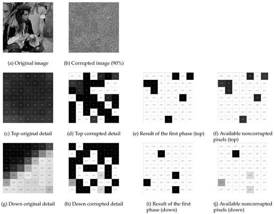
Figure 1.
Two graphical examples of the result of the function described in the noise detection stage introduced in Section 3.1 and the available noncorrupted pixels.
The unavoidable need to use noncorrupted pixels which are quite distant from the central corrupted pixel has an important drawback. The probability that the gray-level value of an arbitrary noncorrupted pixel is close to the original gray-level value of a noisy pixel decreases when the distance between them increases. Therefore, the closer a noncorrupted value is to the corrupted pixel, the more reliable is its value and its influence must be higher in the output. This is certainly the case in the original detail of Figure 1c.
However, this idea does not hold in certain cases. For instance, near an edge, depending on its direction, closer pixels can have distant gray-level values when compared to the central pixel as long as they are located at the other side of the edge. See for instance Figure 1g which corresponds to a detail located near the arm of the man where an edge divides a black region and a lighter region. After applying the first phase of the algorithm, only four pixels are classified as noncorrupted and can be used for restoring the corrupted center pixel (see Figure 1i). Pixel with value 7 is closer than pixel with value 163 although this latter pixel has a more similar value to the centre pixel. Nevertheless, taking into account that (i) edges constitute a small part of the image and (ii) the impossibility to detect edges in images with a high percentage of salt-and-pepper noise, the proposed algorithm will follow that general rule.
The implementation of the previous idea can be easily done by using an aggregation function that applies weights to the noncorrupted input pixels based on how far the input pixel is from the corrupted pixel which is currently being processed. In this paper, a weighted arithmetic mean function (WAM), introduced in Definition 2, is considered. Let us describe the method to compute the weights of the WAM operator. Let be the pixel that is going to be processed and be the noncorrupted pixels which will be aggregated to reconstruct . Please note that depends on the pixel , and the only requirement that we impose is that it must exceed n, which is the least number of non-noisy pixels that are going to be considered to restore . The formula of the aggregation function is as follows:
where the weights for all are given by
where and the d is a distance on . Please note that these weights are based on an exponential decay with respect to the distance between the available non-noisy pixel and the pixel that is currently being processed. This ensures that if this distance increases, the weight of the noncorrupted pixel in the final output is smaller.
It is evident that the performance of the filter relies heavily on (i) the least quantity of non-noisy pixels considered in the aggregation function, which is denoted by n, (ii) on the exponential base of the weights, and (iii) on the considered distance, d. In Section 4.3, an in-depth analysis of the optimal values of these three parameters according to the noise level is included.
Let us explain how the search of those pixels designated as noncorrupted (at least n) is implemented to restore a concrete corrupted pixel . Let and take into account the set of all the noncorrupted pixels whose distance to is . If a minimum of n non-noisy pixels are found, no more iterations are necessary and these pixels will be aggregated by using Equation (2). Otherwise, D is incremented by 1 and the search resumes. This step ends when enough non-noisy pixels are found. It is clear that the search step does depend on the considered distance. In Figure 2, the evolution of the search window for each of the distances considered in Section 4.3 is displayed.
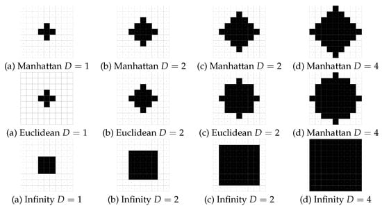
Figure 2.
Evolution of the search window (in black) of noncorrupted pixels for some values of D in a image and three different distances.
Summarising the filtering stage, let A be the corrupted image, b the image computed in step 3) of Algorithm 2, n the minimum number of non-noisy pixels to perform the aggregation, the base of the exponential function considered in the weights and d the selected distance. For each corrupted pixel detected by the noise detection function, the following steps are carried out:
| Algorithm 2: (Filtering Phase) |
|
From now on we will denote this filter as the adaptive weighted arithmetic mean, AWAM for short.
4. Comparison Experiments and Analysis
In this section, first, we will describe the image database that we used in the visual and numerical experiments. To find the best parameter configuration of the proposed filter, we will explain how we divided the image database into the training and test sets. Next, we will present the performance measures to compare the filters considered in this work. The last part of this section will be devoted to the description of the considered filters and the numerical and visual results of the experiments.
4.1. Image Database
To analyse the performance of the proposed filter, a set of experiments were carried out over a set of 44 images. We selected the 36 natural images that belong to the miscellaneous set of the USC-SIPI image database developed by the University of Southern Carolina. This image database is publicly available at http://sipi.usc.edu/database/misc.tar.gz. Moreover, some well-known images that are usually used in noise removal: barbara, cameraman, elaine, goldhill, lenna, tiffany and two test images lenna with gray rectangles and bycicle test have also been included into the database. Applying salt-and-pepper noise (where 255 means salt and 0 means pepper) with the same probability leads to the generation of the database for the comparison experiments. Specifically, densities from 5% to 95% with a step of 5% were considered as well as a final 98% density and applied to each of the images of the database.
Given that the proposed filter depends on the parameters n, and d, we need to divide the set of 44 images into two subsets: the training set and the test image set. With the training set, as we will explain in Section 4.3, we will find the best parameter configuration for our filter. Then, the test set will be used to compare the performance of the AWAM filter setting the optimal configuration, found with the training set, with respect to several filters that will be presented in Section 4.4. With this procedure, a fair comparison is achieved.
More specifically, 26 of the 44 images (≈) are chosen as the training set and the remaining 18 (≈) as the test set. The choice of all these images has been made randomly by setting a randomization seed.
4.2. Performance Measures
In addition to the visual comparison of the results obtained by the filters, the restoration performance should be measured using several quantitative performance measures. The objective evaluation of the quality of the results is of great importance when an image must be restored or its noise reduced. For this reason, a set of measures which are representative of the state of the art were used. We selected and used four measures, Mean-Squared Error (), Mean Structural Similarity Index Measure (M-SSIM), Peak Signal-to-Noise Ratio - Human Visual System (PSNR ), and Visual Information Fidelity (VIF). The first two measures are widely used, and PSNR and VIF were introduced more recently with the aim to incorporate the human visual system (HSV) in the metric. The code for these metrics are freely accessible and can be used by any researcher. The M-SSIM code can be found in http://live.ece.utexas.edu/research/quality/ssim/ or in https://ece.uwaterloo.ca/~z70wang/research/ssim/. The code for PSNR is accessible in http://ponomarenko.info/psnrhvsm.htm. The code for VIF can be found in http://live.ece.utexas.edu/research/quality/index.htm. A brief overview of each selected metric is presented below.
Hereinafter, we will denote by the noise-free original image, on which some restoration filter has been used. Let be the output of the restoration filter. MSE is computed using the following equation:
This metric is computed solely on differences among pixels and sometimes its results are very far from those perceived by the HSV. Lower MSE values are an indication of better capabilities of the considered filter. In contrast, Structural Similarity Index Measure (SSIM) was defined in [27] under the assumption that human visual perception is highly adapted to extract structural information from a scene. The measure is computed as follows:
where , , , are the means and variances of the images and respectively, is the covariance between and , and . This is a mathematically defined performance measure for grayscale images, which does not incorporate a model of the human visual system. This measure incorporates the three main characteristics of the images: contrast, luminance, and structure, in order to compare the noise-free original image with the restored image . In [27,28] the authors state that for image quality assessment, it is more appropriate to apply the index locally rather than globally. They use a windowing approach, computing local statistics within a square window, which moves pixel-by-pixel over the entire image, and then use the mean to evaluate the quality of the restored image. Namely,
where is the value of when the image is restricted to the local window j (L local windows in total). To compute the SSIM values in this paper we will consider the default parameter values as are established in [27]. This measure takes values in and higher values correspond to better capabilities of the used filter.
To avoid the issues related with the performance of , together with the M-SSIM, two different measures were added to our set of performance measures, the PSNR and the VIF measures, because they improve the correlation with subjective quality judgement taking into account the HSV.
The PSNR quality index is presented by Egiazarian et al. in [29] and it is based on the HVS and . This measure considers a scanning window with the aim of removing mean shift as well as contrast stretching in a similar way to the measure presented in [28]. The PSNR quality index is then calculated using the next expression:
where is defined as follows (see [30]):
where are the image dimensions, , is the Discrete Cosine Transform (DCT) coefficients of the block such that the coordinates of its left upper corner are equal to i and j for the original and distorted image respectively, and is the matrix of correcting factors ([29]). The units of this performance measure are dB and the performance of the filter is higher as larger values of PSNR are obtained.
Sheikh and Bovik in [31] proposed the VIF metric which is based on a HVS model. The main idea of the VIF index is to measure the loss of human-perceivable information in the distortion process. The construction of the VIF index is based on a statistical model for natural scenes, a model for image distortions, and a HVS model in an information-theoretic setting, and it is derived from a quantification of mutual information quantities [31]. Sheikh and Bovik studied the VIF properties and they note that for all practical distortion types, VIF takes values in . Again, higher values correspond with better capabilities of the used filter. They show that , and that if this means that all information from the original image has been lost in the restored image. The authors pointed out that if the VIF is applied to the original image and to a linear contrast enhancement of it with no added noise, then VIF returns a value larger than unity. To compute the VIF measure we follow the steps outlined in [31].
4.3. Parameter Selection
In this section, some experiments are carried out to determine the best parameter values of the algorithm according to the considered performance measures.
4.3.1. Noise Detection Function
The performance of the AWAM noise detection function was deeply studied in [14] according to the values of the threshold t. In this section, a comparison with other known noise detection functions is performed. Namely, the noise detection functions introduced in [2] (OCS), [3] (Fabijanska) and [13] (c-FMMOCS) are considered and their performance is compared with respect to two configurations of the AWAM noise detection function: both with ; and , i.e., the minimum t-norm and its residual implication, the Gödel implication, given by
B a flat structuring element with an squared shape of size 5 (a matrix of 255 values) and one with and the other one with . To evaluate the performance we compute the values of , Accuracy and the False Positive Rate (FPR) obtained by the aforementioned noise detection functions in the training set images, as three examples of well-known performance measures in binary classification tasks. In Figure 3 we show the evolution of the mean value of these measures with respect to the noise density. It is clear from the figure that both configurations of the AWAM noise detection functions outperform heavily the other noise detection functions at low noise densities while all the noise detection functions obtain similar results for high densities. Therefore, we will consider the configuration with as the best configuration of the parameters for this noise detection function.

Figure 3.
Plots of the means of several measures obtained by the considered noise detection functions versus noise density.
4.3.2. Noise Filter
Using the performance measures introduced in Section 4.2 and the training set of images, we found the best parameters of the AWAM filter for each level of noise between and . These parameters are:
- d,
- the considered distance, where corresponds to Manhattan distance, , to Euclidean distance and , to infinity distance.
- ,
- the value of the exponential base of the weights in Expression (3).
- n,
- the number of noncorrupted pixels in the neighborhood of the considered pixel needed in order to do the aggregation.
To find the optimal values of the parameters, a 3-D grid of possible values of the three parameters is considered, where , , (It is possible that the algorithm is unable to find the minimum quantity of non-noisy pixels to restore a noisy pixel even when the search window increases till the whole image. This will happen when the algorithm is applied to small images corrupted with high-density noise. In this case, the WAM operator is applied to the non-noisy pixels that were found even when the minimum quantity has not been reached). The and n values included in the grid were chosen in order to guarantee a reasonable exponential decay of the weights of the WAM operator and a reasonable minimum quantity of nonnoisy pixels to aggregate to restore a noisy pixel. For each similarity measure, and for each value of the grid, we find the mean of the values of the similarity measure for all the images of the training database and we select the value of the grid that obtains the best mean value for this similarity measure. The optimal value of these parameters for each noise level are shown in Table 1. As seen in the table, as the noise level increases, the optimal value of the parameter n also grows according to all the considered similarity measures. On the contrary, for M-SSIM and MSE performance measures, the best value of the parameter also grows as the noise level increases to approximately 75%-85% but then decreases as the noise level reaches 98%. On the other hand, for PSNR and VIF similarity measures, it remains constant at until the value of the noise level is approximately 85% and then the optimal values decrease until the noise level reaches 98%. The best distance corresponds mainly to the Manhattan distance for MSE, PSNR and VIF performance measures. For M-SSIM performance measure, there is no clear difference between the Manhattan and the Euclidean distances since in approximately half of the noise levels, the best distance chosen is the Manhattan distance and, in the rest, the Euclidean distance. Anyway, the infinity distance is never used in the estimation of the best parameters of the proposed algorithm.

Table 1.
Best parameters values d, and n for each noise level according to the considered measures.
At this point, the set-up of the AWAM filter has been completed and a flow chart of the algorithm including the parameter values is depicted in Figure 4.
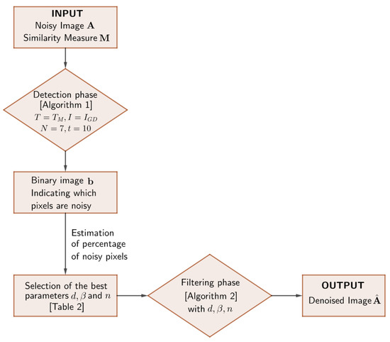
Figure 4.
Flow chart of the AWAM filter with the recommended parameter values.
4.4. Statistical and Visual Comparison with the State-of-the-Art Filters
To evaluate the performance of the AWAM filter, a collection of the most representative state-of-the-art filters for salt-and-pepper noise removal has been chosen. These filters are based on very different approaches and parameters trying to find out the best algorithm that removes the salt-and-pepper noise of the corresponding noisy image:
- SMF5. The classical median filter with a window size of 5 × 5.
- AMF9 and AMF17. AMF stands for Adaptive Median filter and two configurations are considered depending on the maximum allowed size (9 or 17) of the neighborhood window for each pixel.
- DBA. The decision-based filter for highly corrupted images by salt-and-pepper noise proposed by Srinivasan and Ebenezer in [1]. The method changes only corrupted pixels by the median value or by the preceding restored neighboring pixelvalue.
- OCS and OCSFlat. The nonlinear filter based on Open-Close sequence of the classical gray-level morphology. This filter was designed by D. Ze-Feng et al. in [2]. Depending if the structuring element is flat or non-flat, two different versions of the filter were considered.
- c-FMMOCS and c-FMMOCSFlat. The nonlinear filter based on Open-Close sequence within the fuzzy gray-level Mathematical Morphology introduced in [13]. Also, two different filters were considered depending on the type of the structuring element.
- i-FMMOCS and i-FMMOCSFlat. Two versions of the so-called improved Fuzzy Mathematical Morphology Open-Close Filter recently introduced in [14] depending on the choice of the structuring element (non-flat or flat).
- Toh. The two-stage algorithm named noise adaptive fuzzy switching median filter based on fuzzy logic introduced in [8].
- Fabijańska. An algorithm developed in [3] designed to reduce salt-and-pepper noise for extremely corrupted images via analysing local intensity extrema and a median filter.
- Jourabloo. A two-stage filter designed to restore extremely corrupted images with salt-and-pepper noise presented in [4]. In this filter, a noisy pixel is replaced using a non-fixed median filter computed in a window of maximum size of 9, or by estimating the value of the pixel using the values of their neighbors.
- Hosseini. The algorithm designed by Hosseini and Marvasti in order to perform a fast restoration of natural images corrupted by high-density impulsive noise presented in [32].
- AhmedDas. A two-stage adaptive iterative fuzzy filter for denoising images corrupted with high-density salt-and-pepper noise proposed in [33]. In this filter, the detection of noisy pixels is performed with an adaptive fuzzy detector followed by denoising using a weighted arithmetic mean filter, with weights expressed as a potential function of the Euclidean distance between the pixel to be restored, and a set of selected noncorrupted pixels in the filter window.
- Wang. The filter proposed in [5] classifies pixels into three categories: uncorrupted pixels, lightly corrupted pixels, and heavily corrupted pixels, through the maximum absolute luminance difference. In the filtering stage, a weighted average value of the weighted mean of some neighboring pixels and the original pixel value is used to reconstruct the corrupted pixels.
All of them were implemented following the descriptions and parameter values recommended in the original contributions.
The next step is to determine the best filter according to the considered performance measures and to analyse if this filter significantly outperforms the others. Recall that the images in the test set were corrupted using a sequence of 5% to 95% noise levels with a 5% step and 98% noise level. Each considered filter has been applied to all the noisy images. For each filter and noise level, we computed the values of the similarity measures for all the images in the test set. Next, for each pair of filters, the p-value of a paired Wilcoxon signed-rank test based on a 95% confidence level was calculated. From these p-values of these tests, we obtained which filter achieves the finest results, i.e., we found the filter that surpasses the other filters taking into account the statistical test. Table 2 displays those filters that have achieved the best results. If one filter is included in a row, it means that it stands out (as previously explained) for the performance measure indicated in the column and the noise density included in each cell. The color code indicates whether or not the filter significantly surpasses the competitors. For example, according to all the measures, the AWAM filter significantly overcomes the competitors for the 20% noise density, whereas although it always obtains the greatest mean value for the 35% noise, it does not significantly overcome the Hosseini filter (according to M-SSIM and MSE) or the Wang filter (according to PSNR and VIF).
Table 2.
Densities of salt-and-pepper noise for which the row filter is not surpassed by any of the rest in accordance with the Wilcoxon test. A green cell implies that the filter obtains the greatest mean value for that noise density, significantly outperforming the competitors in accordance with the Wilcoxon test. On the other hand, a lime cell implies that although the filter achieves the greatest mean value for that noise density, the difference is not significant according to the Wilcoxon test with respect to those filters coloured in yellow.
As it can be seen, the AWAM filter stands out in almost all the noise densities and in all the performance measures. Furthermore, in a non-negligible quantity of the cases, it is significantly the best among the considered filters. In 28 of the 80 cases, the AWAM filter significantly outperforms the others; in 25 cases, it stands out but not significantly and in only 6 cases, there is another filter that significantly outperforms the others. These 6 cases correspond to low or medium noise levels: 5% (2 cases), 10%, 40%, 50% and 55% (one case). In short, in approximately 66% of the cases, the AWAM filter outperforms the others and this performance is significant in more than half.
Table 3 and Table 4 show the means and standard deviations using the performance measure PSNR of the filters considered for all noise densities. The meaning of the color of the cells is similar to the meaning of the color of the cells of Table 2. The AWAM filter corresponds to the last row and 9 of the 20 possibles boxes, are coloured green and 10 in lime. It means that the AWAM filter almost always outperforms all others filters and in all noise levels. More specifically, in 9 of the 20 noise levels, it significantly outperforms all other filters and in 10, it outperforms them but not significantly.
Table 3.
PSNR average values and standard deviations of the studied algorithms for the sequence of densities of noise from to with a step of . For a concrete density, green cells mean that the filter gets the highest average value, significantly surpassing the competitors; lime cells mean that the filter achieves the highest average value but its results are not statistically different from the ones obtained by the filters depicted in yellow.
Table 4.
PSNR average values and standard deviations of the studied algorithms for the sequence of densities of noise from to with a step of and .
Figure 5 shows the plots of the evolution of the PSNR means depending on the noise densities for each filter. For most of the noise densities, the AWAM filter is positioned at the top of the other filters displaying the best results. For the other performance measures, the conclusions are similar.
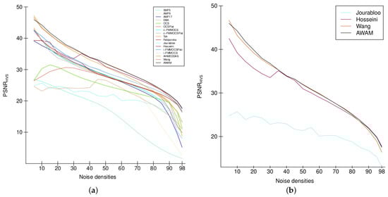
Figure 5.
Graphical evolution of the means of the PSNR values obtained by all the filters in the test set versus noise density. (a) Complete figure. (b) Figure including only those filters that obtain the best results in general according to Table 2.
In summary, the AWAM filter represents a significant advance in the salt-and-pepper noise removal with respect to the existing filters in the literature.
From the above statistical analysis, we conclude that AWAM improves the results of the other algorithms from the numerical point of view. Anyway, we will analyse visually the results given by some of the algorithms comparing them visually to the ones obtained by the proposed AWAM filter.
To develop this visual comparison, the Hosseini and the Wang algorithms were chosen due to their numerical performance. First, Figure 6 shows the results of these filtering algorithms for the image 7.1.02.tiff (which is an aerial photograph of a plane in a hanger) that has been corrupted with 20%, 40%, 60% salt-and-pepper noise. It can be observed that the Hosseini algorithm has a bad performance when the noise is 60%, obtaining as a result an image with undesirable blurred areas. Besides, the values of the PSNR are lower than the values obtained by the AWAM filter. With respect to the results of the Wang filter, they are very similar to the ones obtained by the AWAM filter. In this case, the performance of both filters is very similar.
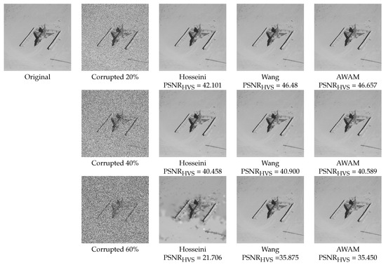
Figure 6.
Restoration results, including the PSNR values, of Hosseini, Wang and AWAM filters for the original image 7.1.02.tiff (an aerial photograph of a plane in a hanger) corrupted with 20%, 40% and 60% salt-and-pepper noise.
A second experiment was performed on the image I11.tiff (a test image of a bicycle and some other elements such as a clock, a plant and a tennis racket) which was corrupted with 80%, 90%, 95%, and 98% salt-and-pepper noise. The corrupted images were filtered with the Hosseini, the Wang and the AWAM filters. Results can be observed in Figure 7. In this case the results given by the Hosseini filter are very blurry and from the 90% to the 98% noise levels, the outputs of the filter are full of spots, leading to a bad visual performance. In the case of the Wang filter, for high density noise levels, the results provided by the AWAM and Wang filters are visually different, and it seems like the results obtained by the AWAM filter are slightly better, also shown by the differences of the PSNR values. Indeed, the values of the PSNR measure are lower because the restoration step of the Wang filter involves a lower number of pixels. On the contrary, for the AWAM filter, the visual performance seems more blurred, but the intensity levels are closer to the ones of the original image.
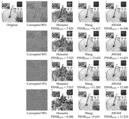
Figure 7.
Restoration results, including the PSNR values, of Hosseini, Wang and AWAM filters for the original image I11.tiff (bycicle test image) corrupted with 80%, 90%, 95% and 98% noise.
Another experiment that was developed involves the study of some details of the output images given by these algorithms. The image 4.1.07.tiff was chosen and corrupted by 60% salt-and-pepper noise. As observed in Figure 8, the edges in the filtered images obtained by the Hosseini filter are not well defined meanwhile in the filtered images by Wang and AWAM they are preserved, although with the AWAM filter the edges have less drastic changes. Some other examples were performed obtaining similar results.
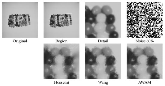
Figure 8.
Restoration results of Hosseini, Wang and AWAM filters for the original image 4.1.07.tiff corrupted with 60% salt-and-pepper noise.
Finally, a visual comparison study was performed with the results obtained by the Wang and AWAM filters for corrupted images with high levels of noise (namely, 80%, 90%, 95% and 98%). In Figure 9 we can observe some of them. In general, the results obtained with the AWAM filter are superior, both from the numerical and and the visual points of view. Since the Wang filter uses fewer pixels in order to restore each pixel of the noisy image, the obtained images look like a piecewise reconstructed image, as observed in the images 4.2.03.tiff and 5.1.09.tiff. On the contrary, the results obtained by the AWAM filter are more realistic, as they do not have these artifacts.
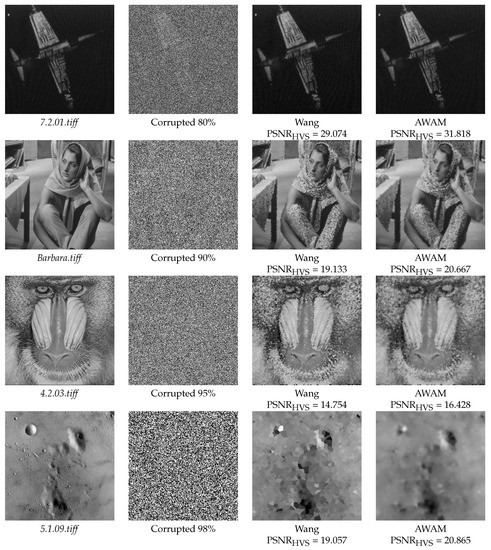
Figure 9.
Restoration results of Wang and AWAM filters when applied to the original images shown in the first column, corrupted with high levels of salt-and-pepper noise.
From all these experiments it can be concluded that the AWAM filter outperforms the results obtained by other filters from the visual point of view.
To end this section, a comparison of the computational processing time of the considered filters is carried out. In Figure 10a, the average computational processing times for the images of the test set are depicted for all the filters and noise densities considered in this section. Figure 10b shows a zoomed version of the previous graph with the vertical range restricted to the interval [0, 1], i.e., average computational processing times smaller or equal to 1 s. From this figure, several conclusions emerge. First, the filters SMF5, AMF9, AMF17, Fabijanska, OCS and OCSFlat have very low average processing times, but they constitute also the worst filters from both the statistical and visual points of view. With respect to the most competitive filters such as AWAM, Jourabloo, Hosseini and Wang, all of them have higher average processing times but still inferior to 1 s for noise densities less than 85%. For noise densities greater than 90%, the computation time of the AWAM filter is higher than most of the other methods but (i) its performance compensates it and (ii) this time could be greatly reduced by parallel computing. The experiments were performed in MATLAB R2020b with a Windows 10 operating system with 16 Gb of RAM memory and an Intel(R) Core(TM) i7-10750H CPU @ 2.60 GHz 2.59 GHz.
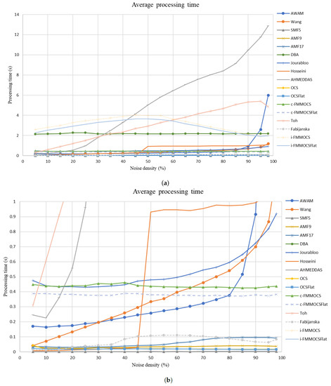
Figure 10.
Evolution of the average computational processing times of all the filters for the images of the test set with respect to the considered noise densities. (a) Complete figure. (b) Zoomed figure for processing times less than 1 s.
5. Conclusions and Future Work
In this work the AWAM filter was presented. This filter is a new salt-and-pepper noise filter that uses a fuzzy mathematical morphology-based noise detection function, followed by an adaptive filtering phase formulated on a weighted arithmetic mean. Two main phases are clearly differentiated: a noise detection phase and a filtering phase. First, a noise detection function classifies each pixel of the image as corrupt or not based on some alternate morphological filters. This detection function is suitable even when a 98% of salt-and-pepper noise has affected an image. In the final phase the gray-level values of those pixels classified as corrupt in the first phase are restored. Given a noisy pixel, its gray-level is restored through an aggregation of the gray-level values of the neighboring noncorrupted pixels by means of an adaptive weighted arithmetic mean operator.
An in-depth evaluation of the performance of the filter is also carried out. The optimal values for the parameters of the AWAM filter were determined for each noise density and performance measure (MSE, M-SSIM, PSNR and VIF) by using a training set. Then, a comparison in a test set whose images had been corrupted with salt-and-pepper noise densities in was made with other 15 top salt-and-pepper noise filters. Both from the visual and numerical standpoints, the proposed filter outperforms all the competition. More specifically, in accordance with the PSNR performance measure, the AWAM filter obtains significantly the best results for 9 noise densities and not significantly for 10 noise densities. Similar results were obtained for the other performance measures.
Finally, the basis of the future work we want to develop is to make some adjustments to the AWAM filter in order to be able to remove general impulsive noise or Gaussian noise.
Author Contributions
Conceptualization, M.G.-H., S.M., A.M. and D.R.-A.; methodology, M.G.-H., S.M., A.M. and D.R.-A.; software, M.G.-H., S.M., A.M. and D.R.-A.; validation, M.G.-H., S.M., A.M. and D.R.-A.; formal analysis, M.G.-H., S.M., A.M. and D.R.-A.; investigation, M.G.-H., S.M., A.M. and D.R.-A.; resources, M.G.-H., S.M., A.M. and D.R.-A.; data curation, M.G.-H., S.M., A.M. and D.R.-A.; writing—original draft preparation, M.G.-H., S.M., A.M. and D.R.-A.; writing—review and editing, M.G.-H., S.M., A.M. and D.R.-A.; visualization, M.G.-H., S.M., A.M. and D.R.-A.; supervision, M.G.-H., S.M., A.M. and D.R.-A.; project administration, M.G.-H., S.M., A.M. and D.R.-A.; funding acquisition, M.G.-H. and S.M. All authors have read and agreed to the published version of the manuscript.
Funding
This work has been partially supported by the Spanish Grant FEDER/Ministerio de Economía, Industria y Competitividad—AEI/TIN2016-75404-P.
Conflicts of Interest
The authors declare no conflict of interest.
References
- Srinivasan, K.; Ebenezer, D. A New Fast and Efficient Decision-Based Algorithm for Removal of High-Density Impulse Noises. IEEE Signal Process. Lett. 2007, 14, 189–192. [Google Scholar] [CrossRef]
- Deng, Z.-F.; Yin, Z.-P.; Xiong, Y.-L. High Probability Impulse Noise-Removing Algorithm Based on Mathematical Morphology. IEEE Signal Process. Lett. 2007, 14, 31–34. [Google Scholar] [CrossRef]
- Fabijańska, A.; Sankowski, D. Noise adaptive switching median-based filter for impulse noise removal from extremely corrupted images. IET Image Process. 2011, 5, 472–480. [Google Scholar] [CrossRef]
- Jourabloo, A.; Feghahati, A.; Jamzad, M. New algorithms for recovering highly corrupted images with impulse noise. Sci. Iran. 2012, 19, 1738–1745. [Google Scholar] [CrossRef]
- Wang, Y.; Wang, J.; Song, X.; Han, L. An Efficient Adaptive Fuzzy Switching Weighted Mean Filter for Salt-and-Pepper Noise Removal. IEEE Signal Process. Lett. 2016, 23, 1582–1586. [Google Scholar] [CrossRef]
- Schulte, S.; De Witte, V.; Nachtegael, M.; Van der Weken, D.; Kerre, E. Fuzzy Two-Step Filter for Impulse Noise Reduction From Color Images. IEEE Trans. Image Process. 2006, 15, 3567–3578. [Google Scholar] [CrossRef] [PubMed]
- Wang, X.; Zhao, X.; Guo, F.; Ma, J. Impulsive noise detection by double noise detector and removal using adaptive neural-fuzzy inference system. Int. J. Electron. Commun. 2011, 65, 429–434. [Google Scholar] [CrossRef]
- Toh, K.; Isa, N. Noise Adaptive Fuzzy Switching Median Filter for Salt-and-Pepper Noise Reduction. IEEE Signal Process. Lett. 2010, 17, 281–284. [Google Scholar] [CrossRef]
- Serra, J. Image Analysis and Mathematical Morphology, Vols. 1, 2; Academic Press: London, UK, 1988. [Google Scholar]
- Bloch, I.; Maître, H. Fuzzy mathematical morphologies: A comparative study. Pattern Recognit. 1995, 28, 1341–1387. [Google Scholar] [CrossRef]
- Nachtegael, M.; Kerre, E. Classical and fuzzy approaches towards mathematical morphology. In Fuzzy Techniques in Image Processing; Kerre, E.E., Nachtegael, M., Eds.; Number 52 in Studies in Fuzziness and Soft Computing; Physica-Verlag: New York, NY, USA, 2000; Chapter 1; pp. 3–57. [Google Scholar]
- González-Hidalgo, M.; Massanet, S.; Mir, A.; Ruiz-Aguilera, D. High-density impulse noise removal using fuzzy mathematical morphology. In Proceedings of the 8th Conference of the European Society of Fuzzy Logic and Technology Conference (EUSFLAT 2013), Milano, Italy, 11–13 September 2013; Pasi, G., Montero, J., Ciucci, D., Eds.; Atlantis Press: Milano, Italy, 2013; pp. 728–735. [Google Scholar]
- González-Hidalgo, M.; Massanet, S.; Mir, A.; Ruiz-Aguilera, D. A Fuzzy Filter for High-Density Salt and Pepper Noise Removal. In Advances in Artificial Intelligence; Bielza, C., Salmeron, A., Alonso-Betanzos, A., Hidalgo, J.I., Martínez, L., Troncoso Lora, A., Corchado, E., Corchado, J.M., Eds.; Lecture Notes in Computer Science; Springer: Berlin/Heidelberg, Germany, 2013; Volume 8109, pp. 70–79. [Google Scholar]
- González-Hidalgo, M.; Massanet, S.; Mir, A.; Ruiz-Aguilera, D. Improving Salt and Pepper Noise Removal Using a Fuzzy Mathematical Morphology-Based Filter. Appl. Soft Comput. 2018, 63, 167–180. [Google Scholar] [CrossRef]
- González-Hidalgo, M.; Massanet, S.; Mir, A.; Ruiz-Aguilera, D. On the Weighted Arithmetic Mean Fuzzy Filter. In Proceedings of the 2015 IEEE International Conference on Fuzzy Systems (FUZZ-IEEE), Istanbul, Turkey, 2–5 August 2015; Pasi, G., Montero, J., Ciucci, D., Eds.; IEEE: Istanbul, Turkey, 2015. [Google Scholar]
- Schulte, S.; De Witte, V.; Nachtegael, M.; Van der Weken, D.; Kerre, E.E. Fuzzy random impulse noise reduction method. Fuzzy Sets Syst. 2007, 158, 270–283. [Google Scholar] [CrossRef]
- De Baets, B. Fuzzy Morphology: A Logical Approach. In Uncertainty Analysis in Engineering and Science: Fuzzy Logic, Statistics, and Neural Network Approach; Ayyub, B.M., Gupta, M.M., Eds.; Kluwer Academic Publishers: Norwell, MA, USA, 1997; pp. 53–68. [Google Scholar]
- González-Hidalgo, M.; Massanet, S.; Mir, A.; Ruiz-Aguilera, D. A fuzzy morphological hit-or-miss transform for grey-level images: A new approach. Fuzzy Sets Syst. 2016, 286, 30–65. [Google Scholar] [CrossRef]
- Baczyński, M.; Jayaram, B. Fuzzy Implications; Studies in Fuzziness and Soft Computing; Springer: Berlin/Heidelberg, Germany, 2008; Volume 231. [Google Scholar]
- Baczyński, M.; Jayaram, B.; Massanet, S.; Torrens, J. Fuzzy Implications: Past, Present, and Future. In Springer Handbook of Computational Intelligence; Kacprzyk, J., Pedrycz, W., Eds.; Springer: Berlin/Heidelberg, Germany, 2015; pp. 183–202. [Google Scholar]
- Klement, E.; Mesiar, R.; Pap, E. Triangular Norms; Kluwer Academic Publishers: London, UK, 2000. [Google Scholar]
- González-Hidalgo, M.; Mir-Torres, A.; Ruiz-Aguilera, D.; Torrens, J. Image Analysis Applications of Morphological Operators based on Uninorms. In Proceedings of the Joint 2009 International Fuzzy Systems Association World Congress and 2009 European Society of Fuzzy Logic and Technology Conference (IFSA-EUSFLAT 2009), Lisbon, Portugal, 20–24 July 2009; Carvalho, P., Dubois, D., Kaymak, U., Sousa, J.M.C., Eds.; EUSFLAT Society: Lisbon, Portugal, 2009; pp. 630–635. [Google Scholar]
- González-Hidalgo, M.; Massanet, S. A fuzzy mathematical morphology based on discrete t-norms: Fundamentals and applications to image processing. Soft Comput. 2014, 18, 2297–2311. [Google Scholar] [CrossRef]
- Beliakov, G.; Pradera, A.; Calvo, T. Aggregation Functions: A Guide for Practitioners; Studies in Fuzziness and Soft Computing; Springer: Berlin/Heidelberg, Germany, 2007; Volume 221. [Google Scholar]
- Grabisch, M.; Marichal, J.L.; Mesiar, R.; Pap, E. Aggregation Functions (Encyclopedia of Mathematics and Its Applications), 1st ed.; Cambridge University Press: New York, NY, USA, 2009. [Google Scholar]
- Singh, A.; Ghanekar, U.; Kumar, C.; Kumar, G. An Efficient Morphological Salt-and-Pepper Noise Detector. Int. J. Adv. Netw. Appl. 2011, 2, 873–875. [Google Scholar]
- Wang, Z.; Bovik, A.C.; Sheikh, H.R.; Simoncelli, E.P. Image Quality Assessment: From Error Visibility to Structural Similarity. IEEE Trans. Image Process. 2004, 13, 600–612. [Google Scholar] [CrossRef] [PubMed]
- Wang, Z.; Bovik, A. A universal image quality index. IEEE Signal Process. Lett. 2002, 9, 81–84. [Google Scholar] [CrossRef]
- Egiazarian, K.; Astola, J.; Ponomarenko, N.; Lukin, V.; Battisti, F.; Carli, M. New full-reference quality metrics based on HVS. In Proceedings of the Second International Workshop on Video Processing and Quality Metrics, Scottsdale, AZ, USA, 22–24 January 2006; Volume 4. [Google Scholar]
- Nill, N. A Visual Model Weighted Cosine Transform for Image Compression and Quality Assessment. IEEE Trans. Commun. 1985, 33, 551–557. [Google Scholar] [CrossRef]
- Sheikh, H.; Bovik, A. Image information and visual quality. IEEE Trans. Image Process. 2006, 15, 430–444. [Google Scholar] [CrossRef] [PubMed]
- Hosseini, H.; Marvasti, F. Fast restoration of natural images corrupted by high-density impulse noise. EURASIP J. Image Video Process. 2013, 2013, 15. [Google Scholar] [CrossRef]
- Ahmed, F.; Das, S. Removal of High-Density Salt-and-Pepper Noise in Images With an Iterative Adaptive Fuzzy Filter Using Alpha-Trimmed Mean. IEEE Trans. Fuzzy Syst. 2014, 22, 1352–1358. [Google Scholar] [CrossRef]


Publisher’s Note: MDPI stays neutral with regard to jurisdictional claims in published maps and institutional affiliations. |
© 2021 by the authors. Licensee MDPI, Basel, Switzerland. This article is an open access article distributed under the terms and conditions of the Creative Commons Attribution (CC BY) license (http://creativecommons.org/licenses/by/4.0/).