Improving the Accuracy of Remote Sensing Land Cover Classification by GEO-ECO Zoning Coupled with Geostatistical Simulation


Abstract
1. Introduction
- (1)
- Taking Geo-Eco zoning as the area of geostatistics. Generally the area of geostatistics is based on the selected image area, which often contains boundary effect, that is, the fact that a class may have statistically biased smaller frequencies of transitions if it has a higher chance of occurring at boundaries of the study area because boundary polygons are incomplete and have no transition to other classes beyond the boundary [28]. Generally, the boundary of Geo-Eco zoning does not cross two different types of land cover to avoid the boundary effect.
- (2)
- In previous research, the large number of sample pixels were interpreted by experts to obtain a transiogram model [28], but this process is time-consuming and laborious. In this study, reliable verification data published by some websites or institutions related to land cover research are reused to reduce the work on visual interpretation.
- (3)
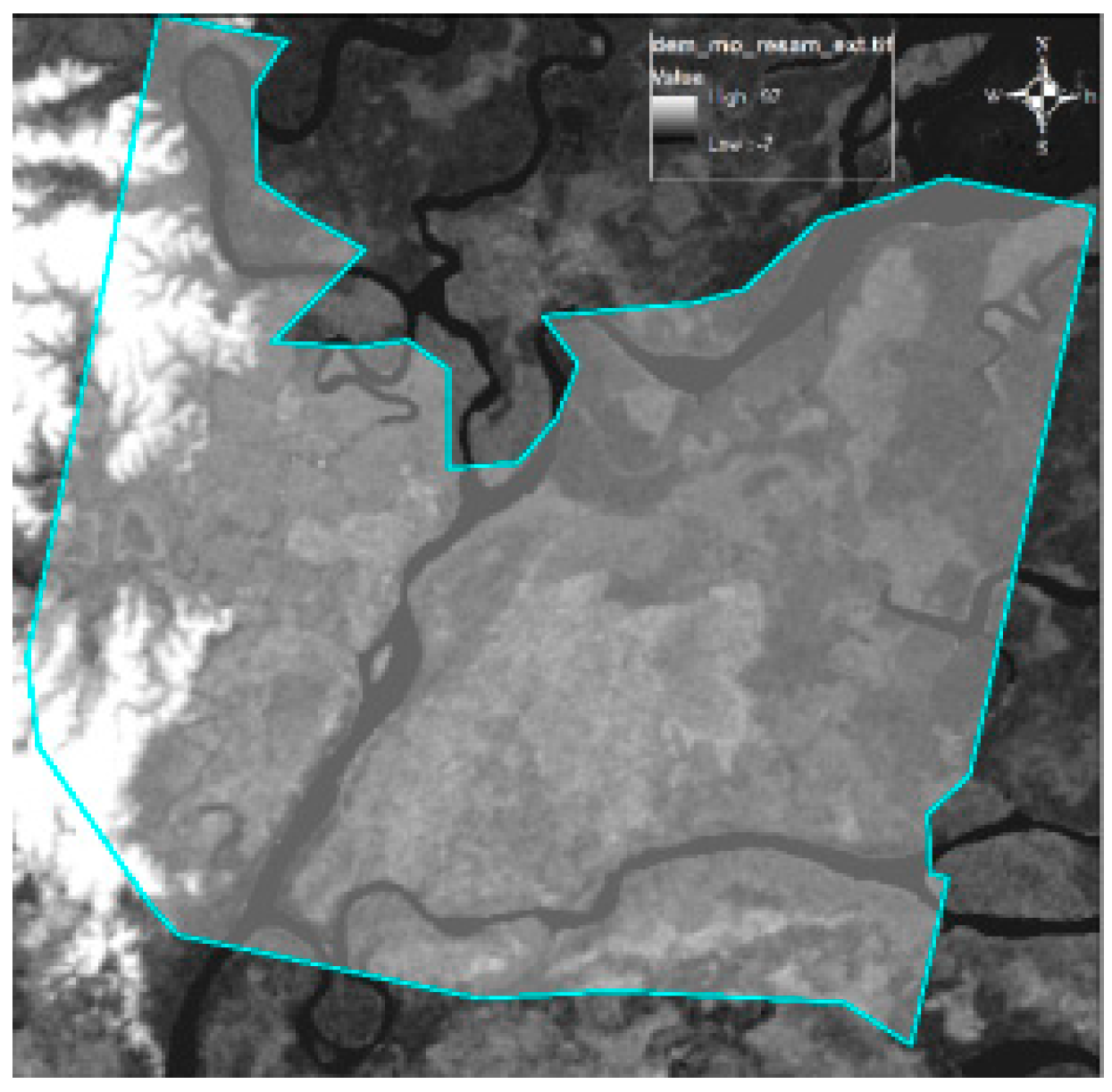
- The Co-MCSS method not only combines remote sensing pre-classified images but also takes various attributes of Geo-Eco zoning (such as DEM, slope, temperature, and humidity) as auxiliary data to participate in the simulation and calculation of cross field transition probability. With the combination of additional attribute information, the simulation algorithm becomes more robust.
2. Method
2.1. Geo-Eco Zoning Rule Base
2.2. Markov Chain Co-Simulation
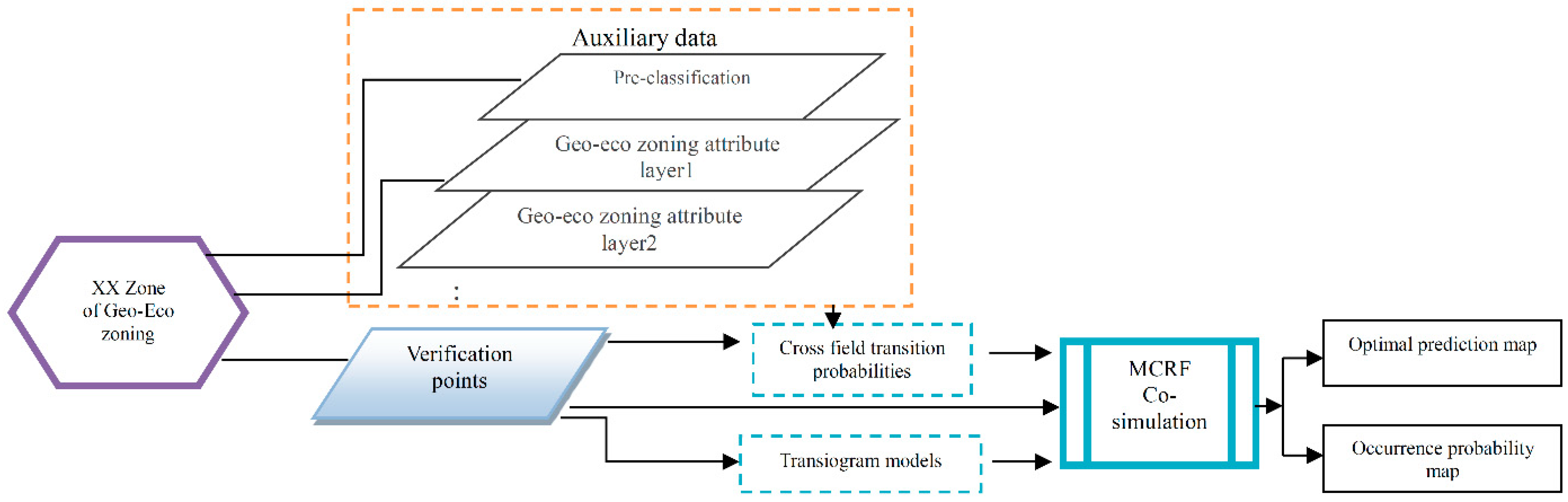
2.2.1. Process
- (1)
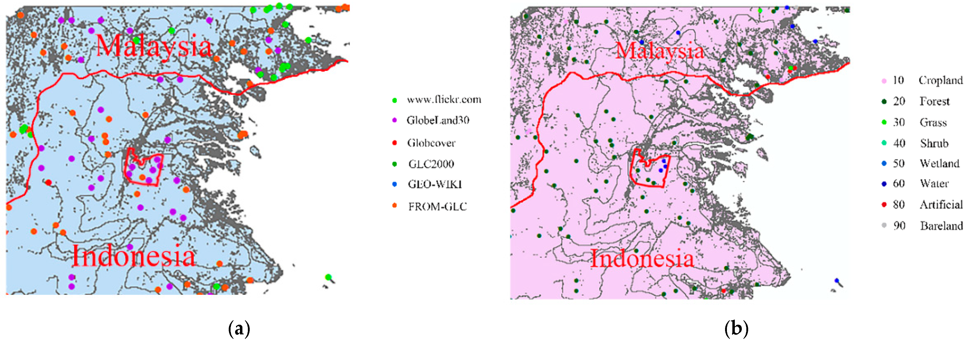
- The land cover verification points from networks were collected from the relevant websites (citations are provided below). If the amount of verification points from networks was not enough for the transiogram estimation, then visual interpretation of sample points was added as a supplement to form the sample data set.
- (2)
- Traditional methods, such as the maximum likelihood method, were used to obtain pre-classified images. The natural attribute layers (such as DEM, slope, and aspect) of Geo-Eco zoning constituted the auxiliary data set for co-simulation.
- (3)
- A set of transiograms were estimated by using the sample data set.
- (4)
- The cross field transition probabilities were estimated by the sample and auxiliary data set.
- (5)
- Co-MCSS algorithm was carried out under the condition of sample data and auxiliary data.
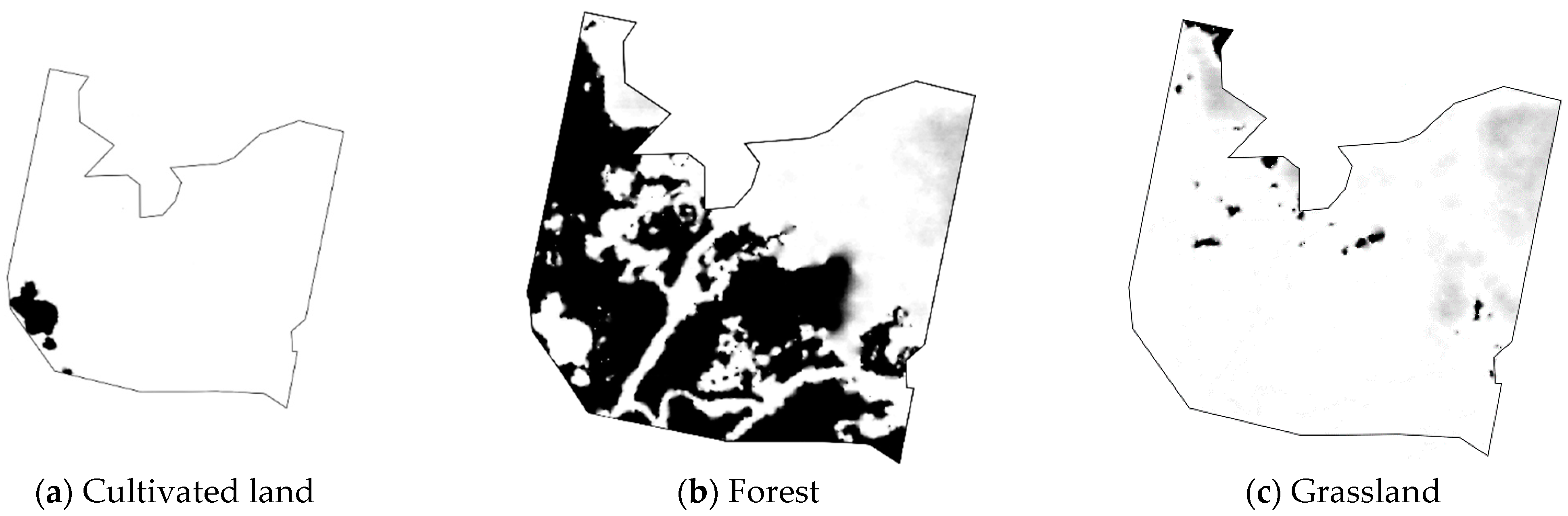
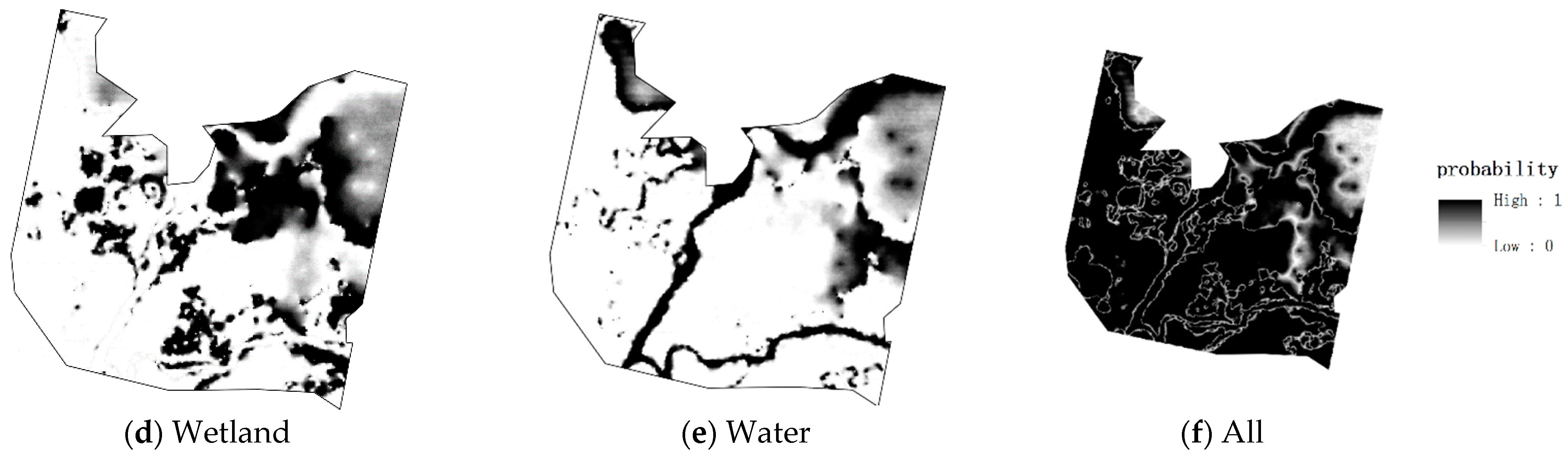
- (6)
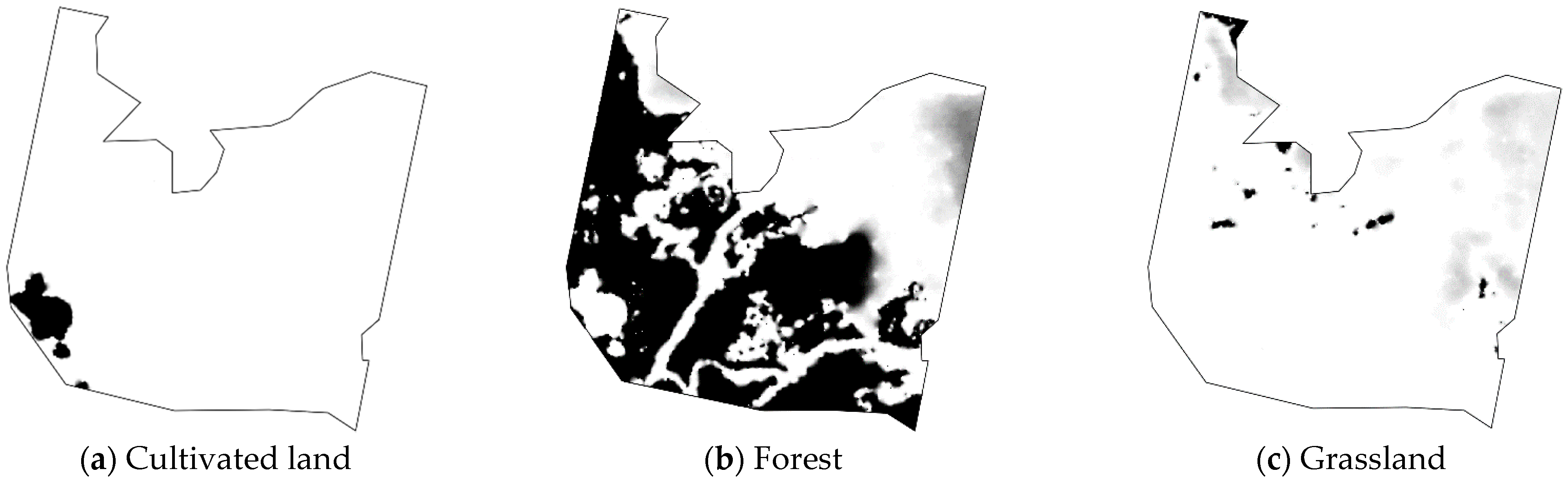
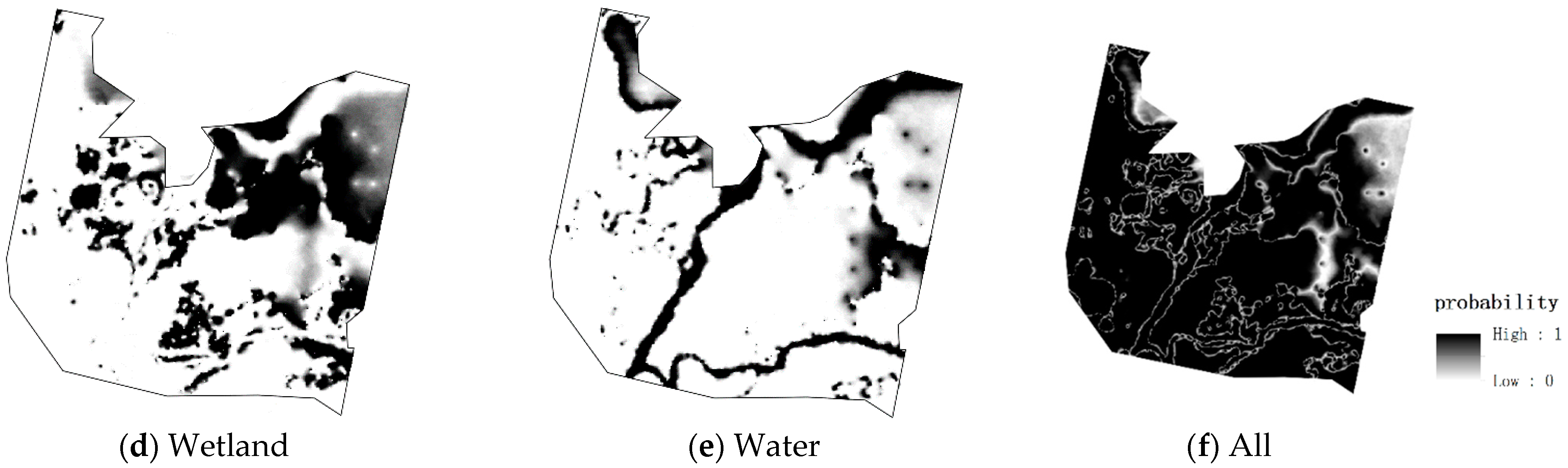
- The optimal prediction map and occurrence probability map were obtained.
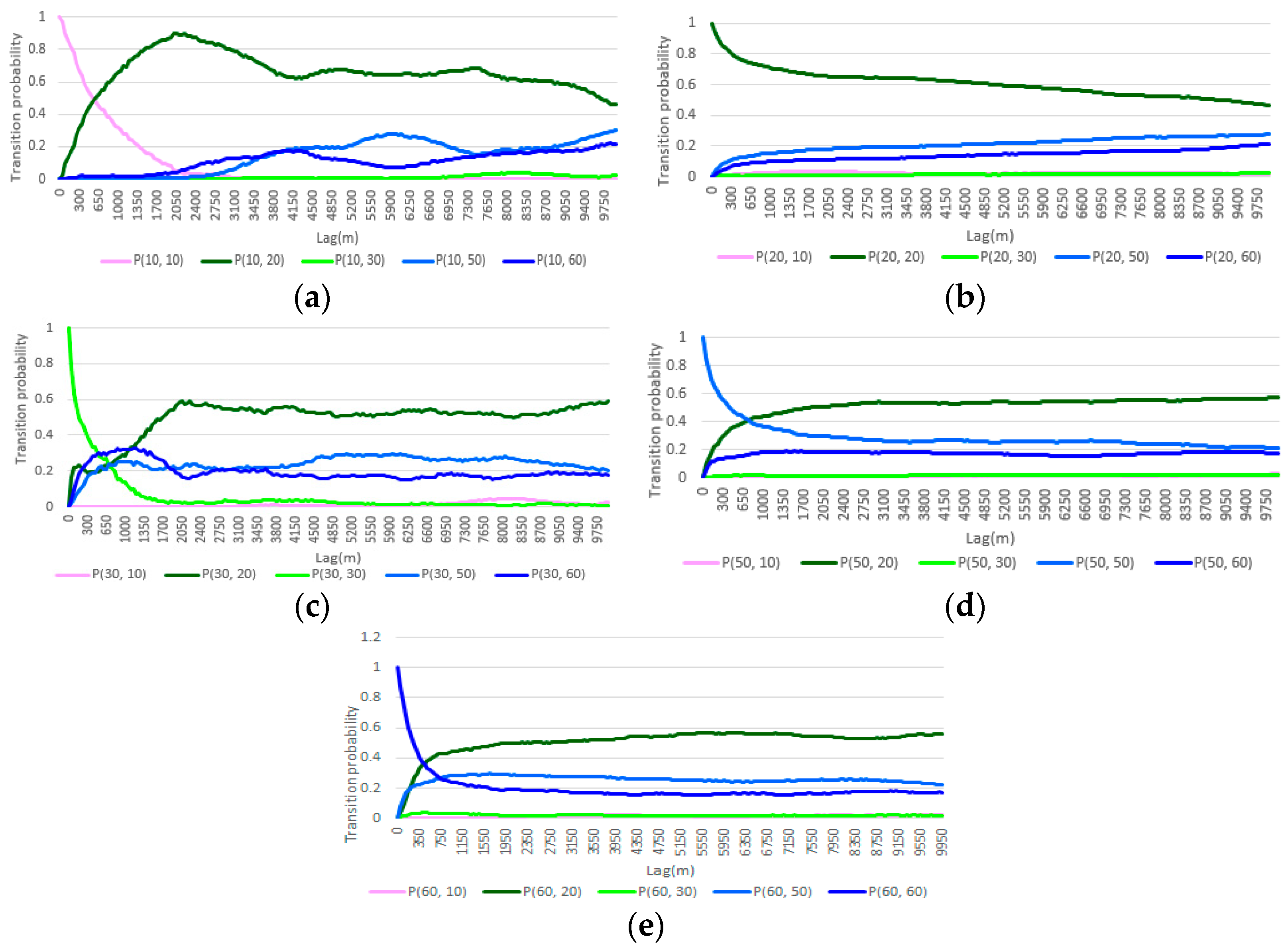
2.2.2. Transiogram
2.2.3. Cross Field Transition Probability Matrix
2.2.4. MCRF Co-Simulation (Co-MCSS)
3. Results
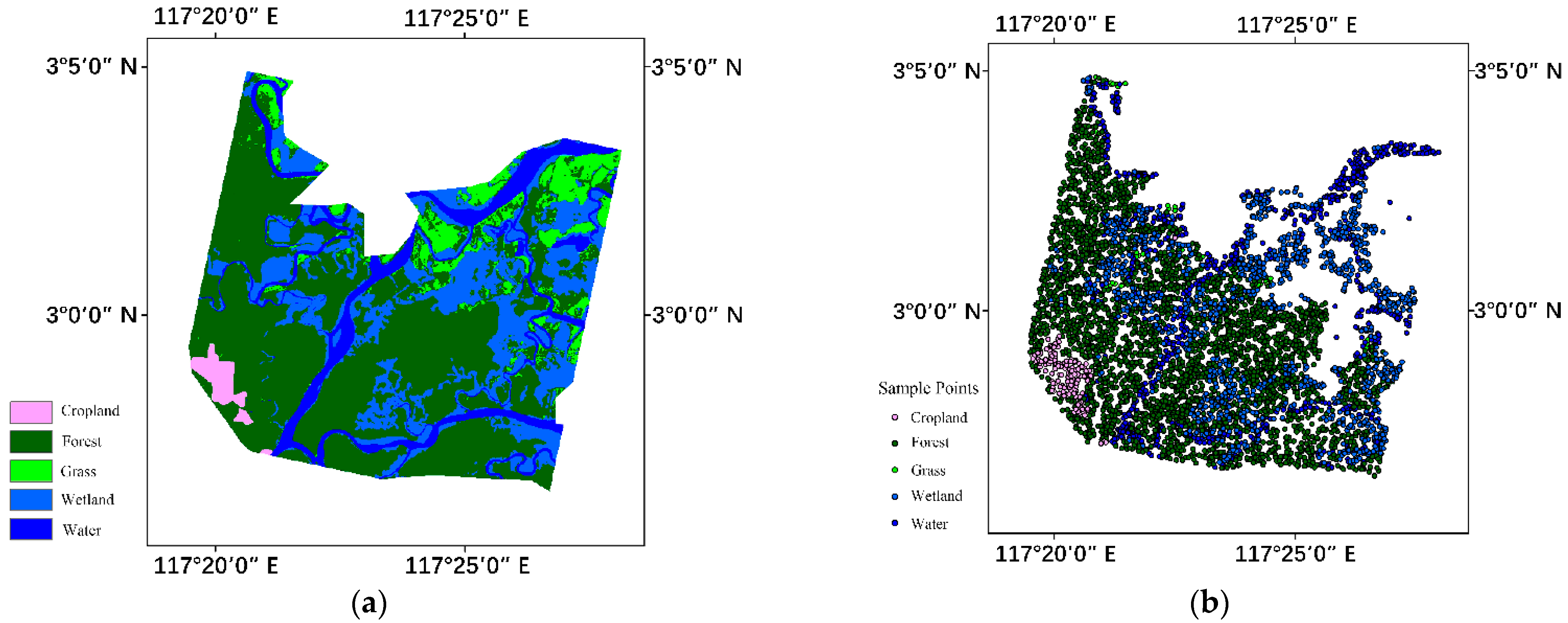
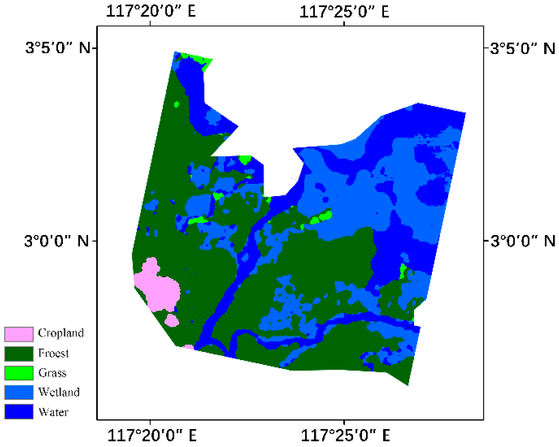
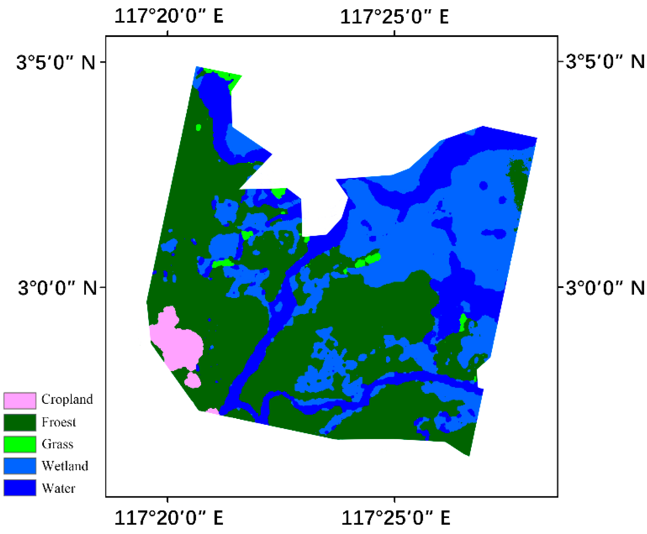
3.1. Study Area
3.2. Transfer Probability Diagram
3.3. Simulation Results
3.3.1. Simulation Results of MCRF
3.3.2. Simulation Results of Co-MCRF with Auxiliary Data
3.4. Accuracy Analysis
4. Conclusions
- (1)
- In this study, the image size that can be processed is limited because of the high operation cost of the algorithm. The experimental area only contains one Geo-eco zone. In future studies, the algorithm should be optimized, and a GPU-parallel acceleration method should be used to increase the amount of data that can be processed and make the algorithm more practical.
- (2)
- Existing data are limited, thus only the attribute data related to elevation are tested, and the impact of other types of auxiliary data are yet to be described. The role of Geo-Eco zoning in geostatistical simulation should be further explored. For example, geoscience knowledge on Geo-Eco zoning can be applied and combined with verification points to generate reasonable transiograms and further reduce the number of sample pixels required by the algorithm.
- (3)
- The case study only tested in one site with a high density of the sample points. The method needs to be verified with a wider scope and more example sites in the future.
Author Contributions
Funding
Institutional Review Board Statement
Informed Consent Statement
Data Availability Statement
Acknowledgments
Conflicts of Interest
References
- Chen, J.; Chen, J.; Liao, A. Remote Sensing Mapping of Global Land Cover; Sci. Press: Beijing, China, 2016. (In Chinese) [Google Scholar]
- Townshend, J.; Justice, C.; Li, W.; Gurney, C.; McManus, J. Global land cover classification by remote sensing: Present capabilities and future possibilities. Remote Sens. Environ. 1991, 35, 243–255. [Google Scholar] [CrossRef]
- Defries, R.S.; Townshend, J.R.G. Global land cover characterization from satellite data: From research to operational implementation? Glob. Ecol. Biogeogr. 1999, 8, 367–379. [Google Scholar] [CrossRef]
- Verburg, P.H.; Neumann, K.; Nol, L. Challenges in using land use and land cover data for global change studies. Glob. Chang. Biol. 2011, 17, 974–989. [Google Scholar] [CrossRef]
- Loveland, T.R.; Reed, B.C.; Brown, J.F.; Ohlen, D.O.; Zhu, Z.; Yang, L.; Merchant, J.W. Development of a global land cover characteristics database and IGBP discover from 1 km AVHRR data. Int. J. Remote Sens. 2000, 21, 1303–1330. [Google Scholar] [CrossRef]
- Hansen, M.C.; Defries, R.S.; Townshend, J.R.G.; Sohlberg, R.A. Global land cover classification at 1 km spatial resolution using a classification tree approach. Int. J. Remote Sens. 2000, 21, 1331–1364. [Google Scholar] [CrossRef]
- Bartholomé, E.; Belward, A.S. GLC2000: A new approach to global land cover mapping from Earth observation data. Int. J. Remote Sens. 2005, 26, 1959–1977. [Google Scholar] [CrossRef]
- Tateishi, R.; Uriyangqai, B.; Al-Bilbisi, H.; Ghar, M.A.; Tsend-Ayush, J.; Kobayashi, T.; Kasimu, A.; Hoan, N.T.; Shalaby, A.; Alsaaideh, B. Production of global land cover data—GLCNMO. Int. J. Digit. Earth 2011, 4, 22–49. [Google Scholar] [CrossRef]
- Arino, O.; Perez, J.R.; Kalogirou, V.; Defourny, P.; Achard, F. GlobCover 2009; Esa Living Planet Symposium: Bergen, Norway, 2010.
- Friedl, M.A.; Sulla-Menashe, D.; Tan, B.; Schneider, A.; Ramankutty, N.; Sibley, A.; Huang, X. MODIS Collection 5 global land cover: Algorithm refinements and characterization of new datasets. Remote Sens. Environ. 2010, 114, 168–182. [Google Scholar] [CrossRef]
- Chen, J.; Cao, X.; Peng, S.; Ren, H. Analysis and Applications of GlobeLand30: A Review. ISPRS Int. J. Geo-Inf. 2017, 6, 230. [Google Scholar] [CrossRef]
- Gong, P. Mapping essential urban land use categories in china (EULUC-China): Preliminary results for 2018. Sci. Bull. 2020, 65, 182–187. [Google Scholar] [CrossRef]
- Giri, C.P. Remote Sensing of Land Use and Land Cover: Principles and Applications; CRC Press: Boca Raton, FL, USA, 2012; pp. 254–255. [Google Scholar]
- Tsendbazar, N.E.; De Bruin, S.; Fritz, S.; Herold, M. Spatial Accuracy Assessment and Integration of Global Land Cover Datasets. Remote Sens. 2015, 7, 15804–15821. [Google Scholar] [CrossRef]
- Liu, T.; Chen, X.; Dong, Q.; Cao, X.; Chen, J. Research on the Application of Deep Learning in GlobeLand30-2010 Product Classification Accuracy Optimization. Remote Sens. Technol. Appl. 2019, 34, 3–11. (In Chinese) [Google Scholar]
- Makoto, N.; Takashi, M. A Structural Analysis of Complex Aerial Photographs; Springer: New York, NY, USA, 1980. [Google Scholar]
- Civco, D. Knowledge-Based Land Use and Land Cover Mapping. In Proceedings of the Annual Convention of American Society for Photogrammetry and Remote Sensing, Baltimore, MD, USA, 16 March 1989; Volume 3, pp. 276–291. [Google Scholar]
- Dobson, M.C.; Pierce, L.E. Knowledge-based land-cover classification using ERS-1/JERS-1SAR composites. IEEE Trans. Geosci. Remote Sens. 1996, 34, 83–99. [Google Scholar] [CrossRef]
- Wentz, E.A.; Nelson, D.; Rahman, A.; Stefanov, W.L.; Roy, S.S. Expert system classification of urban land use/cover for Delhi, India. Int. J. Remote Sens. 2008, 29, 4405–4427. [Google Scholar] [CrossRef]
- Phiri, D.; Morgenroth, J. Remote sensing Review Developments in Landsat Land Cover Classification Methods: A Review. Remote Sens. 2017, 9, 967. [Google Scholar] [CrossRef]
- Chen, J.; Chen, J.; Gong, P.; Liao, A.; He, C. High resolution remote sensing mapping of global land cover. Geomat. World 2011, 9, 12–14. (In Chinese) [Google Scholar]
- Olson, D.M.; Dinerstein, E.; Wikramanayake, E.D.; Burgess, N.D.; Powell, G.W.N.; Underwood, E.C.; D’amico, J.A.; Itoua, I.; Strand, H.E.; Morrison, J.C. Terrestrial ecoregions of the world: A new map of life on Earth. BioScience 2001, 51, 933–938. [Google Scholar] [CrossRef]
- Zhu, L.; Sun, Y.; Shi, R.; La, Y.; Peng, S. Exploiting Cosegmentation and Geo-Eco Zoning for Land Cover Product Updating. Photogramm. Eng. Remote. Sens. 2019, 85, 597–611. [Google Scholar] [CrossRef]
- Van der Meer, F. Remote-sensing image analysis and Geostatistics. Int. J. Remote Sens. 2012, 33, 5644–5676. [Google Scholar] [CrossRef]
- De Bruin, S. Predicting the areal extent of land-cover types using classified imagery and geostatistics. Remote Sens. Environ. 2000, 74, 387–396. [Google Scholar] [CrossRef]
- Carvalho, J.; Soares, A.; Bio, A. Improving satellite images classification using remote and ground data integration by means of stochastic simulation. Int. J. Remote Sens. 2006, 27, 3375–3386. [Google Scholar] [CrossRef]
- Tang, Y.; Atkinson, P.M.; Wardrop, N.A.; Zhang, J. Multiple-point geostatistical simulation for post-processing a remotely sensed land cover classification. Spat. Stat. 2013, 5, 69–84. [Google Scholar] [CrossRef]
- Li, W. Transiogram: A spatial relationship measure for categorical data. Int. J. Geogr. Inf. Sci. 2006, 20, 693–699. [Google Scholar]
- Li, W.; Zhang, C. A Markov chain geostatistical framework for land-cover classification with uncertainty assessment based on expert-interpreted pixels from remotely sensed imagery. IEEE Trans. Geosci. Remote Sens. 2011, 49, 2983–2992. [Google Scholar] [CrossRef]
- Li, W.D.; Zhang, C.; Willig, M.R.; Dey, D.K.; Wang, G.; You, L. Bayesian Markov Chain Random Field Cosimulation for Improving Land Cover Classification Accuracy. Math. Geosci. 2015, 47, 123–148. [Google Scholar] [CrossRef]
- Li, W. Transiograms for Characterizing Spatial Variability of Soil Classes. Soil Sci. Soc. Am. J. 2007, 71, 881–893. [Google Scholar] [CrossRef][Green Version]
- Xing, H.; Chen, J.; Zhou, X. A Geoweb-Based Tagging System for Borderlands Data Acquisition. ISPRS Int. J. Geo-Inf. 2015, 4, 1530–1548. [Google Scholar] [CrossRef]
- Mayaux, P.; Eva, H.; Gallego, J.; Strahler, A.H.; Herold, M.; Agrawal, S.; Naumov, S.; De Miranda, E.E.; Di Bella, C.M.; Ordoyne, C. Validation of the global land cover 2000 map. IEEE Trans. Geosci. Remote Sens. 2006, 44, 1728–1739. [Google Scholar] [CrossRef]
- Bontemps, S.; Defourny, P.; Bogaert, E.V.; Santoro, M.; Kirches, G.; Wevers, J.; Boettcher, M.; Brockmann, C.; Lamarche, C. GlobCover—Products Description and Validation Report. Available online: https://epic.awi.de/ (accessed on 22 November 2020).
- Friedl, M.A.; McIver, D.K.; Hodges, J.C.F.; Zhang, X.Y.; Muchoney, D.; Strahler, A.H.; Woodcock, C.E.; Gopal, S.; Schneider, A.; Cooper, A. Global land cover mapping from MODIS: Algorithms and early results. Remote Sens. Environ. 2002, 83, 287–302. [Google Scholar] [CrossRef]
- Friedl, M.A.; Muchoney, D.; McIver, D.; Gao, F.; Hodges, J.C.F.; Strahler, A.H. Characterization of North American land cover from NOAA-AVHRR data using the EOS MODIS land cover classification algorithm. Geophys. Res. Lett. 2000, 27, 977–980. [Google Scholar] [CrossRef]
- Olofsson, P.; Stehman, S.V.; Woodcock, C.E.; Sulla-Menashe, D.; Sibley, A.M.; Newell, J.D.; Friedl, M.A.; Herold, M. A global land-cover validation data set, part I: Fundamental design principles. Int. J. Remote Sens. 2012, 33, 5768–5788. [Google Scholar] [CrossRef]
- Zhao, Y.Y.; Gong, P.; Yu, L.; Wang, X. Towards a common validation sample set for global land-cover mapping. Int. J. Remote Sens. 2014, 35, 4795–4814. [Google Scholar] [CrossRef]


| Color | Code | Land Cover Type |
|---|---|---|
 | 10 | Cropland |
 | 20 | Forest |
 | 30 | Grass |
 | 40 | Shrub |
 | 50 | Wetland |
 | 60 | Water |
 | 80 | Artificial |
 | 90 | Bareland |
| Simulation Method | Number of Matching | Proportion |
|---|---|---|
| Pre-classified image (GlobeLand30-2015) | 5962 | 75.34% |
| Simulation results of MCRF | 6451 | 81.52% |
| Simulation results (with auxiliary data) | 6843 | 86.48% |
Publisher’s Note: MDPI stays neutral with regard to jurisdictional claims in published maps and institutional affiliations. |
© 2021 by the authors. Licensee MDPI, Basel, Switzerland. This article is an open access article distributed under the terms and conditions of the Creative Commons Attribution (CC BY) license (http://creativecommons.org/licenses/by/4.0/).
Share and Cite
Zhu, L.; Li, J.; La, Y.; Jia, T. Improving the Accuracy of Remote Sensing Land Cover Classification by GEO-ECO Zoning Coupled with Geostatistical Simulation. Appl. Sci. 2021, 11, 553. https://doi.org/10.3390/app11020553
Zhu L, Li J, La Y, Jia T. Improving the Accuracy of Remote Sensing Land Cover Classification by GEO-ECO Zoning Coupled with Geostatistical Simulation. Applied Sciences. 2021; 11(2):553. https://doi.org/10.3390/app11020553
Chicago/Turabian StyleZhu, Ling, Jing Li, Yixuan La, and Tao Jia. 2021. "Improving the Accuracy of Remote Sensing Land Cover Classification by GEO-ECO Zoning Coupled with Geostatistical Simulation" Applied Sciences 11, no. 2: 553. https://doi.org/10.3390/app11020553
APA StyleZhu, L., Li, J., La, Y., & Jia, T. (2021). Improving the Accuracy of Remote Sensing Land Cover Classification by GEO-ECO Zoning Coupled with Geostatistical Simulation. Applied Sciences, 11(2), 553. https://doi.org/10.3390/app11020553